

1. Introduction
Cervical cancer is one of the most common malignant cancer of women in developing countries, so that various medical studies have been carried out to reduce the incidence and the mortality rates, see [12] and [15]. Developing the Human Papilloma Virus (HPV) vaccines and cervical screening studies are very important to prevent and to eliminate the spreads of cancer cells, see [10] and [11].
There are some studies of cervical cancer in the perspective of mathematics, such as, the effectiveness of the HPV vaccine, immunotherapy model of cervical cancer at the cellular level, metastasis' behaviour model of cervical cancer in the tissue level, and the global stability analysis for a cervical cancer model, see [16], [18], [6], [4], [17], and [2]. The implementation of control functions to the model has been done in [13] and [5], where the authors apply a combination of drug therapies and controlling the number of precancerous cells to reduce the growth of the cancer. Meanwhile, in [1], the authors applied control theory in two cell populations, i.e., susceptible cells and virus population. Based on the fact that the virus' infection to the cells is depend on the maturity of the cells, the authors in [8], [9], [19] developed an age-structured model for cervical cancer.
In mathematical perspective, the studies of cancer are focused to understand the characteristics of cancer's spreads in the cellular level and the effectiveness of the vaccinations and treatments. They consider the existence and stability of the non endemic and the endemic equilibrium points that represent the spread of the cancer cells, and the behaviour of the cells populations with respect to time numerically. However, in most cases, not all behaviour of the solution near the endemic equilibrium points have been studied.
In [4], the authors introduced a model for cervical cancer that show the interaction between normal cells (S), infected cells by HPV (I), free HPV (V), precancerous cells (P), and cancer cells (C), which is simply called SIVPC model, and studied the equilibrium points where the existence depend on the basic reproduction
*Corresponding author
Received February 8<sup>th</sup>, 2024, Revised June 14<sup>th</sup>, 2024 (first), Revised September 21<sup>st</sup>, 2024 (second), Accepted for publication December 20<sup>th</sup>, 2024. Copyright ©2024 Published by Indonesian Biomathematical Society, e-ISSN: 2549-2896, DOI:10.5614/cbms.2024.7.2.8
ratio. In [3], the authors found the appearance of the cusp bifurcation in a certain parameter space of the SIVPC model.
Our study is the sequel work of [4] and [3]. We consider the existence conditions of a nontrivial equilibrium point, which does not depend on the basic reproduction ratio. In application, the appearance of this equilibrium point is important to understand the conditions for the effective treatments in the high stadium of the cancer cases. The sensitivity analysis and the numerical bifurcation analysis regarding to the parameter variations are also studied in this paper. The studies are important to characterize the cancer' spreads and the possibility to determine the irregular behaviour based on the parameter space of the model.
We start this paper by the brief introduction of the SIVPC model and the basic reproduction ratio, and then study the existence conditions of a nontrivial equilibrium point of the model that do not depend on the basic reproduction ratio. After that, we do continuation of some parameters and analyze the bifurcation of the system numerically. In this case, we will show some interesting bifurcations that can be used to indicate the irregular behavior of the system. Lastly, we will close the discussion with the sensitivity analysis of some parameters and the concluding remarks.
2. PROBLEM FORMULATION
Consider the SIVPC model for cervical cancer on [4], cervical cells divided into four sub-populations which are susceptible cells (S), infected cells (I), pre-cancer cells (P) and cancer cells (C). The free Human Papillomavirus compartment (V) also included on this model. The growth of susceptible cells describe by logistic function with intrinsic growth rate r and decreased while susceptible cells infected by human papilomavirus with infection rate \(\alpha\). The growth rate of infected cells, pre-cancer cells and cancer cells respectively given by a,b and k. By persistent infection, the infected cells will be progress become precancerous cells with progression rate \(\delta\) and pre-cancer cells progress into cancer cells with maximum progression rate \(\theta\). The number of free virus will be increase from the infected cells and decrease with clearance rate c. The system of differential equation given on system (1) with definition of parameters are given on Table 1.
\[\frac{dS}{dt} = rS(1 - (S + I)) - \alpha SV,\] \[\frac{dI}{dt} = \alpha SV - (a + \delta)I,\] \[\frac{dV}{dt} = nI - cV,\] \[\frac{dP}{dt} = \delta pI + bP - \theta \frac{P^2}{1 + P^2},\] \[\frac{dC}{dt} = \theta \frac{P^2}{1 + P^2} - kC.\] (1)
Table 1: Parameters and units.
| Symbol | Explanation of parameter | Unit |
|---|---|---|
| \(\overline{r}\) | intrinsic growth rate of susceptible cells | 1/day |
| \(\alpha\) | infection rate | \(1/(day \times number of virus)\) |
| a | growth rate of infected cells | 1/day |
| \(\delta\) | progression rate from infected to precancerous | 1/day |
| n | average number of virions produced by an infected cell | constant |
| c | clearance rate of free virus | 1/day |
| b | growth rate of precancerous cells | 1/day |
| \(\theta\) | maximal progression rate from precancerous to cancerous | 1/day |
| k | growth rate of cancer cells | 1/day |
The first three equations are decoupled from the final two, and so the equilibrium values of S, I, and V can be found algebraically, as in [4]. Given an equilibrium \((\overline{S}, \overline{I}, \overline{V})\), we may then attempt to find the equilibrium value of P, and subsequently also the equilibrium value of C. In [4], the five parameter scenarios for the existences of positive (endemic) equilibria are derived by Sturm sequence condition. Here we will directly solving \(\frac{dP}{dt} = 0\) to find the equilibrium, assuming a known value for \(\overline{I}\). We adopt the values of \(\overline{I}\) and \(R_0 = \frac{\alpha n}{c(a+\delta)}\) from [4].
3. EXISTENCE OF THE NON-TRIVIAL EQUILIBRIUM
In the previous article [4] several scenarios for the existence of the equilibrium points of System (1) were given, focusing on the conditions for the existence of a non-negative real equilibrium point. In this section we will provide a theorem that guarantees the existence of an equilibrium point by looking at the analytical solution and focusing on the real solution conditions.
Theorem 3.1. Consider \(A = \frac{\delta p(\alpha nc^2 - (a+\delta)c^3)}{c^2 + \alpha n}\), \(F = -8A^3 + 24A^2\theta - 72Ab^2 - 24A\theta^2\), \(G = 4A^2 - 12A^3\theta + 8A^2b^2 + 12A^2\theta^2 + 20Ab^2\theta - 4A\theta^3 + 4b^4 - b^2\theta^2\), and \(H = 36b^2\theta - 8\theta^3\). There are seven equilibrium points of the model, i.e.
- 1) \(E_1 = (0,0,0,0,0)\) and \(E_4 = (1,0,0,0,0)\) that exist for every condition,
- 2) \(E_{2.3} = \left(0, 0, 0, P_{1.2}, \frac{\theta b}{k}\right)\) and \(E_{5.6} = \left(1, 0, 0, P_{1.2}, \frac{\theta b}{k}\right)\) that exist if \(\theta \le -2b\) or \(\theta \ge 2b\), 3) \(E_7 = \left(\frac{(a+\delta)c}{\alpha n}, \frac{\alpha nc^2 (a+\delta)c^3}{c^2 + \alpha n}, \frac{\alpha n^2c (a+\delta)nc^2}{c^2 + \alpha n}, P_3, \frac{bP_3}{k} + \frac{\delta p(\alpha nc^2 (a+\delta)c^3)}{k(c^2 + \alpha n)}\right)\) that exists if \(\alpha \ge \frac{(a+\delta)c}{n}\), \(G \ge 0\), and \(P_3 \ge 0\),
\(P_{1,2} = \frac{\theta \pm \sqrt{\theta^2 - 4b^2}}{2b}\) and
\[P_{3} = \frac{4A^{2} - 2\left(F + 12\sqrt{3}\sqrt{G}b - H\right)^{1/3}A - 8A\theta + \left(F + 12\sqrt{3}\sqrt{G}b - H\right)^{2/3} + 2\left(F + 12\sqrt{3}\sqrt{G}b - H\right)^{1/3}\theta - 12b^{2} + 4\theta^{2}}{6b\left(F + 12\sqrt{3}\sqrt{G}b - H\right)^{1/3}}.\]
Proof: Equilibrium points are obtained by solving \(\frac{dS}{dt} = \frac{dI}{dt} = \frac{dV}{dt} = \frac{dP}{dt} = \frac{dC}{dt} = 0\). By operating the equation \(\frac{dV}{dt} = 0\), we found \(V = \frac{nI}{c}\). By substituting the value of V to the equation \(\frac{dI}{dt} = 0\), we obtained \(\frac{\alpha nSI}{c} - (a + \delta)I = 0\) which is fulfilled if I = 0 or \(S = \frac{(a + \delta)c}{\alpha n}\). If I = 0, we found \(V = \frac{nI}{c} = 0\). By substituting I = V = 0 to the equation \(\frac{dS}{dt} = 0\), we obtained rS(1 - S) = 0 which implies S = 0 or S = 1. When we substitute I = V = S = 0 to the equation \(\frac{dP}{dt} = 0\), we found \(bP - \frac{\theta P^2}{1 + P^2} = 0\) which is satisfied if P = 0 or \(b = \frac{\theta P}{1 + P^2}\). If we substitute P = 0 to the equation \(\frac{dC}{dt} = 0\), we obtained C = 0. Thus, we found \(E_1 = (0,0,0,0,0)\). When we substitute \(b = \frac{\theta P}{1 + P^2}\) to to the equation \(\frac{dC}{dt} = 0\), we obtain \(C = \frac{\theta b}{k}\). By solving \(b = \frac{\theta P}{1 + P^2}\) we have \(P_{1,2} = \frac{\theta \pm \sqrt{\theta^2 - 4b^2}}{2b}\). Hence, we found \(E_{2,3} = (0,0,0,P_{1,2},\frac{\theta b}{k})\). For S = 1, we also have three pairs of P and C, i.e. P = C = 0 and \(P = P_{1,2}\) with the value of C for those two C is \(C = \frac{\theta b}{k}\). Thus, we obtained C = 0, we found \(C = \frac{\alpha nc^2 - (a + \delta)c^3}{c^2 + \alpha n}\). By substituting the value of C to the equation C = 0 and C = 0 and C = 0. By substituting the value of C = 0 and C = 0. By substituting the value of C = 0 and C = 0. By substituting the value of C = 0 and C = 0 and C = 0. By substituting the value of C = 0 and C = 0 and C = 0 and C = 0 and C = 0 and C = 0 and C = 0 and C = 0 and C = 0 and C = 0 and C = 0 and C = 0 and C = 0 and C = 0 and C = 0 and C = 0 and C = 0 and C = 0 and C = 0 and C = 0 and C = 0 and C = 0 and C = 0 and C = 0 and C = 0 and C = 0 and C = 0 and C = 0 and C = 0 and C = 0 and C = 0 and C = 0 and C = 0 and C = 0 and C = 0 and C = 0 and C = 0 and C = 0 and C = 0 and C = 0 and C = 0 and C = 0 and C = 0 and C =i.e. \(P_{3.4.5}\) and \(\frac{\theta P^2}{1+P^2} = bP + \delta P \left( \frac{\alpha nc^2 - (a+\delta)c^3}{c^2 + \alpha n} \right)\). One root of the cubic equation is in \(\mathbb{R}\), i.e. \(P_3 = \frac{4A^2 - 2(F + 12\sqrt{3}\sqrt{G}b - H)^{1/3}A - 8A\theta + (F + 12\sqrt{3}\sqrt{G}b - H)^{2/3} + 2(F + 12\sqrt{3}\sqrt{G}b - H)^{1/3}\theta - 12b^2 + 4\theta^2}{6b(F + 12\sqrt{3}\sqrt{G}b - H)^{1/3}}\). The other two roots of are in \(\mathbb{C}\), so that they are not exist in \(\mathbb{R}\), i.e. \(P_{4.5}\). By substituting the value \(\frac{\theta P^2}{1+P^2}\) to the equation \(\frac{dC}{dt}=0\), we found \(C = \frac{bP}{k} + \frac{\alpha nc^2 - (a+\delta)c^3}{k(c^2 + \alpha n)}\). By substituting the value of \(P_3\) to the value C, we found \(C = \frac{bP_3}{k} + \frac{\alpha nc^2 - (a+\delta)c^3}{k(c^2 + \alpha n)}\). Therefore, we found \(E_7 = \left(\frac{(a+\delta)c}{\alpha n}, \frac{\alpha nc^2 - (a+\delta)c^3}{c^2 + \alpha n}, \frac{\alpha n^2c - (a+\delta)nc^2}{c^2 + \alpha n}, P_3, \frac{bP_3}{k} + \frac{\delta p(\alpha nc^2 - (a+\delta)c^3)}{k(c^2 + \alpha n)}\right)\). Every equilibria exists if every subpopulation in the equilibria expression is defined in \(\mathbb{R}\) and has a nonnegative value. \(E_1\) and \(E_4\) exist for every condition, because every subpopulation already has defined in \(\mathbb R\)and has a non-negative value. Existence of \(E_2, E_3, E_5\), and \(E_6\) depend on the value of \(P_{1.2}\) while the other subpopulation already have a non-negative value. \(P_{1.2}\) are defined in \(\mathbb{R}\) if \(\theta^2 - 4b^2 \ge 0\) which is satisfied if \(\theta \leq -2b\) or \(\theta \geq 2b\). If those condition is satisfied, then the value of \(P_{1.2}\) is always positive, because \(\theta > \sqrt{\theta^2 - 4b^2}\). Hence, \(E_2, E_3, E_5\), and \(E_6\) exist if \(\theta \leq -2b\) or \(\theta \geq 2b\). \(E_7\) exists if \(\alpha nc^2 - (a+\delta)c^3 \geq 0\), \(\alpha n^2c - (a+\delta)nc^2 \geq 0\), and \(P_3 \geq 0\) in order to guarantee that the infected, virus, and pre-cancer subpopulations have a non-negative value. Beside that, the value of G must also be non-negative in order to guarantee that the value of pre-cancer subpopulation is defined in \(\mathbb{R}\). The first two inequalities are equivalent to \(\alpha \geq \frac{(a+\delta)c}{n}\).
4. BIFURCATIONS OF SOME TREATMENT PARAMETERS
Parameter c, \(\delta\), and b are important, because they have an opportunity to become a treatment target. We set initial values of the parameters according to [4] and make some continuation of the stable equilibrium point by varying those parameters to analyze the codimension one and two bifurcations.
4.1. Fold and Hopf Bifurcations
Continuation of the stable equilibrium point by varying c and \(\delta\) generates Fold and Hopf bifurcations in co-dimension one bifurcation analysis, see Figure 1. Note that H represents Hopf bifurcation, LP represents Fold bifurcation, and BP represents Branch Point.
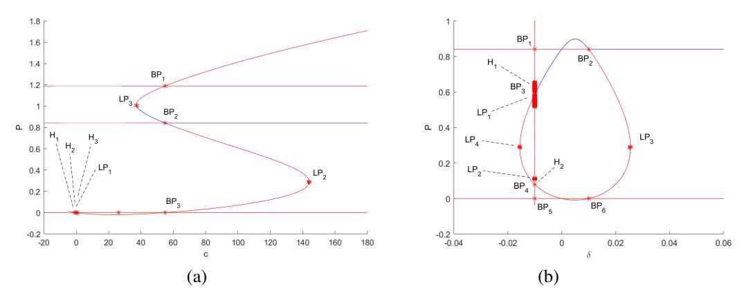
Figure 1: The Fold and Hopf Bifurcations: (a) Hysteresis Constructed by Two Fold Bifurcations as c Varies, (b) Fold Bifurcations Constructed as \(\delta\) Varies.
.
Backward and forward continuation of the stable equilibrium point by varying c generate some bifurcation. Series of Fold bifurcation is found at \(LP_1\), two Fold bifurcations are obtained at \(LP_2\) when c=143.961734 and \(LP_3\) when c=37.3174420887747. Three Hopf bifurcations are found, i.e. at \(H_1\) when c=-1.0378734, \(H_2\) when \(c=5.017633\times 10^{-5}\), and \(H_3\) when c=0.96322656. Three Branch Point bifurcations occur at c=54.945055, see Figure 1(a).
Four equilibrium points are detected when the value of c is less than the value of c at the first Fold point. We found five equilibrium points at the first Fold point as c increases. When the value of c increases beyond the first Fold point and less than the Branch Point, we found six equilibrium points until the Branch point. We obtain three equilibrium points at the Branch point and the equilibrium points become six again as c increases beyond the Branch point until the second Fold point. At the second Fold point, there are five equilibrium points and they collapse become four equilibrium points again same as the number of equilibrium points in the initial condition when the value of c pass through the second Fold point. The occurrence of the Fold bifurcations trigger a hysteresis as an indicator of catastrophe dynamic, whereas the Hopf bifurcations generate a periodic solution at every Hopf bifurcation points which represents a cycle of the cell transformation. The Pitchfork bifurcations represent the merging points of some equilibrium points.
In Figure 1(b), independent with the branch points, two Fold bifurcations occur when we make a backward and forward continuation of the stable equilibrium point by varying \(\delta\), i.e. at \(\delta = -0.015479\) and \(\delta = -0.015479\) and \(\delta = -0.015479\) and \(\delta = -0.015479\) and \(\delta = -0.015479\) and \(\delta = -0.015479\) and \(\delta = -0.015479\) and \(\delta = -0.015479\) and \(\delta = -0.015479\) and \(\delta = -0.015479\) and \(\delta = -0.015479\) and \(\delta = -0.015479\) and \(\delta = -0.015479\) and \(\delta = -0.015479\) and \(\delta = -0.015479\) and \(\delta = -0.015479\) and \(\delta = -0.015479\) and \(\delta = -0.015479\) and \(\delta = -0.015479\) and \(\delta = -0.015479\)
0.025479. We also found fourteen Hopf bifurcations and five branch points. Three of them are obtained at δ = −0.01 and the others are obtained at δ = 0.01. The continuation of the first branch point generates many Fold bifurcations at δ = −0.01. When the value of δ is less than the value of δ at the first Fold point, there is two equilibrium points. Three equilibria is found at the first Fold point and change become four equilibrium points as the value of δ increases beyond the first Fold point until the first three branch point. At the first three branch point, we found many equilibrium points. When δ increases beyond the first three branch point, there are four equilibrium points until the second branch points which generate two equilibrium points. Four equilibrium points are found as δ increases beyond the second branch point until the second Fold point which is found independently with the branch point. At this point, we found three equilibrium points and they collapse become two equilibrium points as δ increases beyond it. A cycle of the cell transformation is found at the Hopf point and the number of steady state condition change at the branch point.
4.2. Cusp and Bogdanov-Takens Bifurcations
Some Cusp and Bogdanov-Takens bifurcations are found by a backward and forward continuation of the Fold point LP3 at δ = 0.025479 as shown in Figure 1(b) when δ and b are varied in the codimension two bifurcation analysis as the further analysis of the codimension one bifurcation result, see Figure 2.
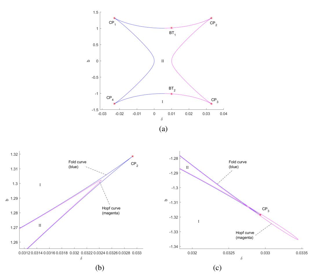
Figure 2: Cusp and Bogdanov-Takens Bifurcations as δ and b Vary: (a) The Cusp and Bogdanov-Takens Bifurcations, (b) Magnification of the Area around CP2, (c) Magnification of the Area around CP3.
.
We make a continuation on the Fold Point (LP3), i.e. δ = 0.025479 generated on codimension-one bifurcation (see Figure 1(b)) as δ and b vary. It generates four Cusp bifurcations (CP1, CP2, CP3, CP4) and two Bogdanov-Takens bifurcations (BT1, BT2), see Figure 2). The Cusp bifurcations occur at (δ, b) = (0.032932, 1.318524), (δ, b) = (0.032932, −1.318524), (δ, b) = (−0.022932, −1.318524), and (δ, b) = (−0.022932, 1.318524) while the Bogdanov-Takens bifurcations occur at (δ, b) = (0.01, 0.002304), (δ, b) = (0.009999, −1.015), (δ, b) = (0.01000003, 1.01500011), and (δ, b) = (0.01, −1.1790965 × 10⁻⁴ ). Two intersecting Fold curves generate Cusp bifurcations as an indication of catastrophe phenomenon. Bogdanov-Takens bifurcations in our system are generated by the intersection of Hopf, Fold, and Homoclinic curves. The Homoclinic curve is an indicator of chaotic dynamic.
To get an illustration of the equilibria stability we plot a phase portrait in area I and area II of Figure 2 and considering for positive δ. While taking δ = 0.005 and b = 0.01, which is in area II, the basic reproduction number R0 is 1.33. In this area there exist 8 equilibrium points and it is according to the previous result in [4]. One equilibria is locally asymptotically stable, and the others are unstable. Figure 3 show that the equilibrium point (0.75, 0.125, 25, 0.06699250312, 0.008980123797) is a locally asymptotically stable.
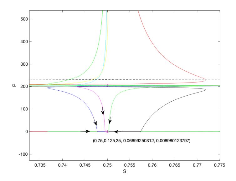
Figure 3: Phase portrait of S-P in area II.
In area I, taking δ = 0.005 and b = −2 also giving the same value of R0 and there exist three equilibrium points. The two equilibrium points are E0 = (0, 0, 0, 0, 0), E1 = (1, 0, 0, 0, 0) which both are unstable. The third equilibrium is E∗ = (0.75, 0.125, 25, 0.004182246755, 0.00003515494103) which is locally asymtotically stable. The phase portrait was given on Figure 4.
From both illustration, it can be seen that there is a difference in the number of equilibrium points in those two areas, even both having the same basic reproduction number. In area I, negative value of b means that the apoptosis rates of pre-cancer cells is larger than the proliferation rates of pre-cancer cells, so the pre-cancer cells population will be decrease. In the medical point of view, this condition giving a bigger change to recover.
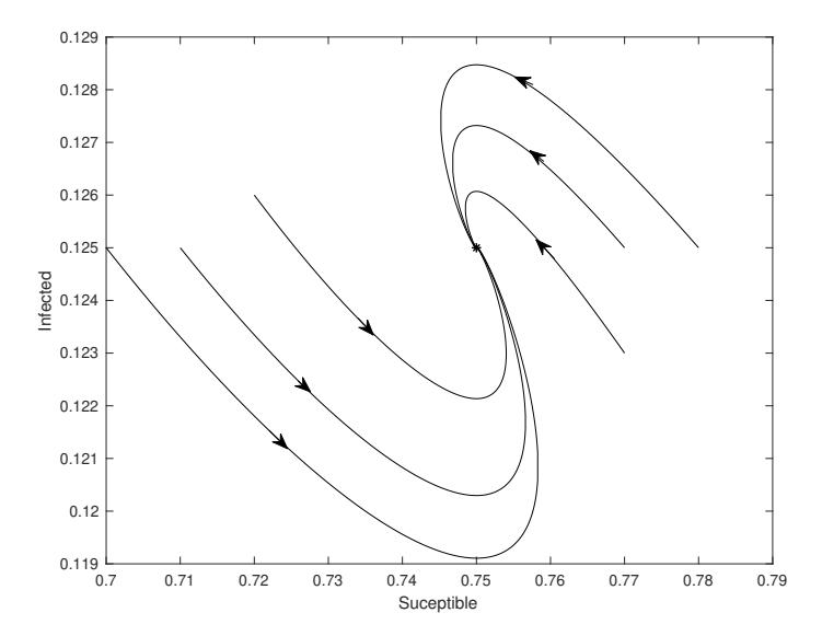
Figure 4: Phase portrait around \(E^*\) of S-I in area I.
5. SENSITIVITY ANALYSIS
For notational convenience, rename the state variables \(X_1 = S\), \(X_2 = I\), \(X_3 = V\), \(X_4 = P\) and \(X_5 = C\). Select a parameter \(\lambda\) from the system of equations, and denote the right hand side of each equation as \(f_i(X_1, \ldots, X_5, \lambda)\), so the system of equations is
\[\frac{dX_i}{dt} = f_i(X_1, \dots, X_5, \lambda), \quad \text{for} \quad i = 1, \dots, 5.\]
At some particular point in the parameter space \(\{r, \alpha, a, \delta, n, c, b, \theta, k\}\), we can calculate the time-dependent sensitivity, \(Z_i\), of each state variable with respect to \(\lambda\). We define
\[Z_i = \frac{\partial X_i}{\partial \lambda}.\]
Each sensitivity variable \(Z_i\) is governed by a differential equation
\[\frac{dZ_i}{dt} = \frac{d}{dt} \cdot \frac{\partial X_i}{\partial \lambda} = \frac{\partial}{\partial \lambda} \cdot \frac{dX_i}{dt} = \frac{\partial}{\partial \lambda} f_i(X_1, \dots, X_5, \lambda)\] \[= \sum_{j=1}^{5} \frac{\partial f_i}{\partial X_j} \cdot \frac{\partial X_j}{\partial \lambda} + \frac{\partial f_i}{\partial \lambda}\] \[= \sum_{j=1}^{5} \frac{\partial f_i}{\partial X_j} Z_j + \frac{\partial f_i}{\partial \lambda}.\]
We will explore the sensitivity of the state variable \(X_4 = P\) with respect to the parameters b and \(\delta\). With \(\lambda = b\), so that \(Z_i = \frac{\partial X_i}{\partial b}\), the differential equations governing the sensitivity variables are
\[\frac{dZ_1}{dt} = (r(1 - 2S - I) - \alpha V) Z_1 - rSZ_2 - \alpha SZ_3, \frac{dZ_2}{dt} = \alpha V Z_1 - (a + \delta) Z_2 + \alpha SZ_3, \frac{dZ_3}{dt} = nZ_2 - cZ_3, \frac{dZ_4}{dt} = \delta pZ_2 + \left(b - \theta \frac{2P}{(1 + P^2)^2}\right) Z_4 + P, \frac{dZ_5}{dt} = \theta \frac{2P}{(1 + P^2)^2} Z_4 - kZ_5,\] (2)
subject to the initial conditions \(Z_i(0) = 0\) for i = 1, ..., 5. To find the time dependent sensitivity \(Z_4(t)\), this system of equations is adjoined to the system of differential equations governing the state variables (1), producing a system of 10 differential equations, which must be solved simultaneously.
To calculate the sensitivity of the state variables to \(\delta\), the adjoined differential equations are changed to
\[\frac{dZ_1}{dt} = (r(1 - 2S - I) - \alpha V) Z_1 - rSZ_2 - \alpha SZ_3, \frac{dZ_2}{dt} = \alpha V Z_1 - (a + \delta) Z_2 + \alpha SZ_3 - I, \frac{dZ_3}{dt} = nZ_2 - cZ_3, \frac{dZ_4}{dt} = \delta pZ_2 + \left(b - \theta \frac{2P}{(1 + P^2)^2}\right) Z_4 + pI, \frac{dZ_5}{dt} = \theta \frac{2P}{(1 + P^2)^2} Z_4 - kZ_5,\] (3)
subject to the initial conditions \(Z_i(0) = 0\) for i = 1, ..., 5. This set of sensitivity equations differs for those with respect to b only in the last term of second and fourth equations.
Because the sensitivities are dependent upon the values of all of the model parameters, we should run simulations of these equations for a few different initial selections of parameter values. At a minimum, we should calculate the sensitivities for a choice of parameters corresponding to progress to cancer, another choice of parameters corresponding to successful treatment, and a third choice representing a patient who would not progress to cancer. We can then compare these to see if there are any noticeable differences. We focus our attention on \(\mathbb{Z}_4\), the sensitivity of the precancerous cell population to the parameter \(\lambda\).
Numerical simulations show that a significant change in the sensitivity \(Z_4(t)\) occurs near b=1 (Figure 5(a)). For b<1, \(Z_4\) remains small for all t. For b>1, \(Z_4\) remains low for approximately 30 days, before rapidly rising to a constant positive value. This behavior persists for larger values of b. This change in sensitivity profile indicates that around b=1, a bifurcation occurs in the in dynamics of precancerous cells. Below this threshold, P is relatively insensitive to the value of b, while above this threshold, P is positively sensitive to b, indicating that P(t) increases as b increases.
Interestingly, the magnitude of the sensitivity to b is largest for b-values that are close to the apparent bifurcation point. From [4] two positive equilibrium will be exist while \(0 < b < \frac{\theta}{2}\) and some certain conditions. In this simulation we are taking \(\theta = 2.03\), so it is make sense that the bifurcation point will appear around b = 1.015.
We next consider \(\lambda = \delta\), the progression rate of infected cells to precancerous cells. In this case, the sensitivity of precancerous cells \((Z_4)\) exhibits a different behavior (Figure 5(b)). For all values of \(\delta\), P shows a high positive sensitivity to \(\delta\) for low t values, which becomes smaller and constant for larger t. For very large t values, a limited period of negative sensitivity occurs, followed by a return to the prior constant value.
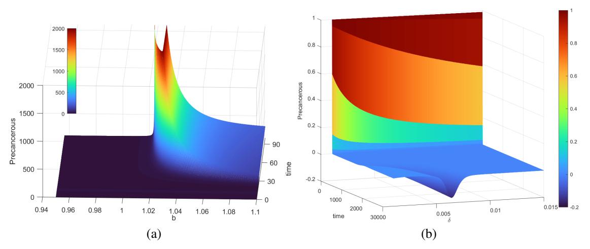
Figure 5: Sensitivity plot of parameter b and parameter δ. (a) Sensitivity plot of parameter b, (b) Sensitivity plot of parameter δ. The color indicates the amount of precancerous cells. The increase in the number of precancerous cells from the lowest to the highest is indicated by dark blue to dark red respectively as written on the colormap.
6. BIOLOGICAL INTERPRETATION
All the results presented above are mathematical results. From a biological or medical point of view, not all of these results can be interpreted. The first is related to parameter variations. In this model, the parameter values that can be interpreted for δ and c are positive values. Parameter δ represents the rate of progression from infected cells to cancer cells, while c represents the rate of death of the virus. Parameter b can be positive or negative, because it represents the growth rate of pre-cancerous cells which is the difference between the rate of proliferation and the rate of apoptosis of pre-cancerous cells. On the other hand, the equilibrium point that can be interpreted is also a positive equilibrium point, considering that each variable describes the density of the sub-population.
Related to this, on the continuation of parameter c, the bifurcation phenomena that can be interpreted biologically is at c = 37.3174420887747 when Fold appears to a value of c = 54.945055 when the Pitchfork bifurcation appears. An endemic equilibrium point exists between these two values. Parameter c describes the clearance rate of free virus with units 1/day. Thus, if condition of the clearance rate of free virus is between 38 and 54 per day, then an endemic equilibrium will be achieved.
For the δ parameter, when the value of δ = 0.01 then the value of R0 = 1. In accordance with the study that has been given in [4], this value becomes the border for the existence of an endemic equilibrium point and its local stability. Thus the bifurcation phenomena that appears at this δ value is in line with the previous results.
On the continuation of two parameters δ and b, compartment S, I and V doesn't depend on b. In this simulation positive value of S, I and V will exist while δ < 0.01. On the other side positive value of P and C exist while b < 1.015. So the possible existence of positive equilibrium point only in two area on Figure 2.
7. CONCLUDING REMARKS
The study of spreads of cervical cancer caused by HPV on the tissue level is important to understand the behavior of the HPV infections in the perspective of mathematics. The paper is a sequel work of [4], [17], and [3] that focus on numerical bifurcations and sensitivity analysis of the system. From this study, we found that there are some bifurcations on the system that trigger the change of the steady state conditions of the system. The appearance of hysteresis and cusp bifurcations on the system, see Figure 1 and Figure 2 show the possibility of the system to have irregular behavior. By understanding the regimes on the parameter space that the system has the irregular behaviour is important to determine the treatment strategy for the disease.
ACKNOWLEDGEMENT
This research was funded by Post Doctoral Program Universitas Gadjah Mada 2021 with Letter of Assignment number 6144/UN1.P.III/DIT-LIT/PT/2021.