

1. INTRODUCTION
The role of human behavior in combating infectious diseases has always been important in epidemic management. This was particularly underscored during the COVID-19 crisis, which emphasized the essential role of disease prevention education and personal protective measures. In the early stages of this pandemic, countries like Italy and Turkey, among the first to experience its impact, implemented relaxed measures based on the evolving situation, leading to severe consequences. Conversely, Morocco, learning from the early experiences of these countries, quickly adopted effective self-protection measures, in the early stages, such as lockdowns, mask-wearing, and social distancing, effectively preventing a surge in case numbers [5].
Late implementation of self-protection measures, as noted in [1], may not significantly curb disease spread, highlighting the need for proactive strategies. Preparedness through ongoing education and awareness campaigns, even in the absence of a local epidemic, can enable the rapid and effective adoption of selfprotection measures that are standard and common for various diseases. This swift adoption can lead to early containment of potential outbreaks, reducing the overall impact on public health and decreasing the burden on healthcare systems.
In epidemiological modeling, introducing a compartment for 'Educated' individuals, who have acquired specific knowledge and behaviors to combat infectious diseases, marks a significant advancement. Various hypotheses have been proposed for recruitment into this class. For example, [12] suggests a linear recruitment rate from the susceptible population, while [13] proposes a constant rate. Other studies, like [8], [9], [1], model the recruitment rate as a function of disease prevalence.
Our study introduces a compartmental epidemiological model to assess how ongoing education and awareness, coupled with sensitization initiated at the epidemic's onset, influence disease prevention. The model employs a dual recruitment method into the 'Educated' class, integrating a constant term ∧ and a variable part W(S, SE, I, R), where S, SE, I and R represent the susceptible, educated, infectious and recovered
*Corresponding author
populations, respectively. The constant term \(\land\) represents enduring education and awareness, independent of the disease's presence, while the variable part \(\mathcal{W}\) reflects behavioral changes in response to the disease's prevalence and severity. Our analysis demonstrates that continuous educational efforts are more effective in disease prevention than initiatives launched after an epidemic's onset, emphasizing the need for proactive strategies.
We apply the model to the influenza epidemic in Nova Scotia, Canada, analyzing data from 2014 to 2017. To reflect the seasonal dynamics of influenza and capture the effects of incubation periods, our model incorporates a periodic coefficient in the force of infection and a delay in the system. These considerations render our model as non-autonomous delayed differential equations, distinguishing it from previously cited works. Some of the model parameters are calibrated to fit the observed real-data and others are estimated using external sources.
The paper is structured to first discuss the mathematical modeling, then the well-posed nature of the model and the basic reproduction number \(R_0\). Section 4 examines the importance of \(R_0\) in understanding disease persistence and potential extinction. Section 5 fits the model to real influenza data from Nova Scotia and deduces \(R_0\). Section 6 assesses the impact of behavioral change on disease spread, examining the sensitivity of \(R_0\) to variables such as seasonality and delay. The paper concludes with a summary of our insights.
2. MATHEMATICAL MODELING
In this work, the mathematical model comprises four compartments: S, \(S_E\), I and R representing the number of susceptible, educated, infected and recovered individuals respectively. The model incorporates two mechanisms for recruitment into the educated class: the first is a constant rate \(\land\), and the second is a variable part W.
The awareness function \(\mathcal{W}\) is activated only when the disease begins, increasing in response to the severity of the situation in terms of human and economic costs. It can be formulated to incorporate factors from within the model, such as the numbers of deaths and recoveries, and external influences like economic variables and health policy recommendations. This formulation provides a broad scope for treating different epidemiological situations. In our specific model, we have chosen to focus \(\mathcal{W}\) exclusively on the variables S, \(S_E\), I and R. This simplifies our model while capturing the essential aspects of individuals transitioning to a more educated state
The \(\wedge\) constant represents education that is not related to the current pandemic. It includes common safety practices such as hand washing, physical distancing, and avoiding crowded places, which are taught through educational channels such as schools, family upbringing, and public awareness campaigns. Through these various methods, these behaviors are introduced early on to young children. Growing up in an educated environment, these children benefit from the collective protection of those around them, naturally joining the educated group \(S_E\) from an early age and remaining in it as they mature. A low value of \(\wedge\) reflects a weak educational system and a lack of effective public awareness efforts, often resulting from less frequent or insufficient health campaigns and limited public health initiatives. This leads to a lower level of awareness and preparedness, potentially delaying the response when an outbreak occurs.
Building on the general description, we now define \(\mathcal W\) analytically. The function \(\mathcal W\) maps the variables \((S,S_E,I,R)\) to \(\mathcal W(S,S_E,I,R)\). It is assumed to take values in the range [0,1], increasing with respect to I and decreasing with respect to I. Additionally, for all I, I, we have I where I we have I there is no recruitment through I into the I class when disease prevalence is zero. As prevalence increases, recruitment into I also rises, demonstrating the model's adaptive response mechanism based on the disease's intensity and impact. Given these properties, we can model the function I using the Hill function of the form:
\[W = \frac{P^n}{(P^*)^n + P^n},\] where \(P=\frac{I}{I+S_E+S+R}\). In this formulation, \(P^*\) represents the prevalence level at which the response function \(\mathcal W\) reaches half of its maximum value. In other words, if \(P=P^*\) then \(\mathcal W=\frac{1}{2}\). The Hill function captures the gradual increase in awareness as the prevalence of the disease rises. Figure 1 illustrates the curve of the Hill function \(\mathcal W(P)\) for different values of \(P^*\) with n=2. The horizontal dashed line at \(\mathcal W(P)=0.5\) indicates the 50% awareness level, while the vertical dashed lines show the corresponding prevalence values where \(P=P^*\) for each curve. A lower \(P^*\) signifies a population that responds quickly to the presence of the disease, with awareness increasing rapidly even at lower prevalence levels. Conversely, a higher P ∗ indicates that a greater prevalence is required to achieve similar awareness levels, reflecting varying degrees of sensitivity to the disease.
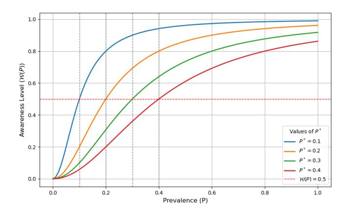
Figure 1: Sensitivity of the awareness function W(P) to disease prevalence P for different threshold values P ∗ .
.
The flow diagram in Figure 2 illustrates the dynamics of the disease, which are mathematically represented in System (1).
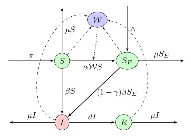
Figure 2: Flow diagram of the model.
\[S'(t) = \pi - \alpha \mathcal{W}(t)S(t) - \beta(t)S(t)I(t) - \mu_1 S(t), \tag{1a}\]
\[S_E'(t) = \Lambda + \alpha \mathcal{W}(t)S(t) - (1 - \gamma)\beta(t)S_E(t)I(t) - \mu_1 S_E(t), \tag{1b}\]
\[I'(t) = e^{-\mu_1 \Delta} \beta(t - \Delta)(S(t - \Delta) + (1 - \gamma)S_E(t - \Delta))I(t - \Delta) - (\mu_2 + d)I(t), \tag{1c}\]
\[R'(t) = dI(t) - \mu_1 R(t). \tag{1d}\]
The function β is positive and ω-periodic. The assumption that individuals exhibit a linear growth rate introduces the survival probability term e −µ1∆ in equation (1c). The remaining model parameters are summarized in Table 1.
Table 1: Definition of parameters.
| Parameter | Definition |
|---|---|
| π | The recruitment rate of susceptible individuals |
| ∧ | Education rate combining inherited and formal learning, covering schooling and |
| alternative educational methods, independent of ongoing disease conditions | |
| ∆ | The incubation period |
| d | Recovery rate for infectious individuals |
| µ1 | Naturel death rate |
| µ2 | ≥ µ1) Death rate due to the infection (µ2 |
| γ | 1 − γ means the efficiency of self protective means |
| α | Maximum of education response |
3. MODEL ANALYSIS
In this section, we first demonstrate that System (1) is well-posed and has biological significance. Secondly, we utilize the method developed in [3] to calculate the basic reproduction number for System (1).
3.1. Well posedness of the model
The initial conditions for System (1) are selected at t = 0 as functions defined over a historical interval, such that
\[(S_0, S_{E_0}, I_0, R_0) = (\varphi_1, \varphi_2, \varphi_3, \varphi_4) \in \mathcal{C}_+^4.\] (2)
where C+ = C([−∆, 0], R+) is the space of continuous and non-negative functions on [−∆, 0].
Lemma 3.1. Assuming that β(t) is a positive, continuous, and periodic function with period ω, the solutions of (1) with initial condition (2) are non-negative and ultimately uniformly bounded.
Proof: Let's begin by proving the non-negativity of S. Suppose, for the sake of contradiction, that S takes a negative value and let t1 be the smallest positive real number such that S(t1) = 0. The existence of t1 is ensured by the continuity of S. From Equation (1a) , we have S ′ (t1) = π > 0. Therefore, for any ϵ > 0 and any t in the interval (t1 − ϵ, t1), we have S(t) > 0. This contradicts the fact that S is negative on [0, t1]. Next, we prove the non-negativity of I and E. Integrating Equation (1c), we obtain:
\[I(t) = e^{-(\mu_2 + d)t}I(0) + e^{-\mu_1 \Delta} \int_0^t e^{-(\mu_2 + d)(t - s)} f(s, S(s - \Delta), S_E(s - \Delta), I(s - \Delta)) ds,\] (3)
where
\[f(t, S, S_E, I) = \beta(t)SI + (1 - \gamma)\beta(t)S_EI.\]
Using the initial conditions (2) and Formula (3), we see that I is non-negative on [0, ∆]. By a similar reasoning used to prove the non-negativity of S, we deduce the non-negativity of SE on [0, ∆]. We repeat this reasoning on intervals of the form [n∆,(n + 1)∆] to deduce the non-negativity of SE and I on R+. Finally, to prove the non-negativity of R, we simply integrate the last equation of the system, taking into account the non-negativity of I.
In the following, we will show that the solution is bounded. Let G(t) = S(t) + SE(t) + e µ1∆I(t + ∆) + e µ1∆R(t + ∆). Using the equations in System (1) and the fact that µ2 ≥ µ1 we get
\[G'(t) \leq \pi + \wedge -\mu_1 \left( S(t) + S_E(t) + e^{\mu_1 \Delta} I(t + \Delta) + e^{\mu_1 \Delta} R(t + \Delta) \right)\]
\[\leq \pi + \wedge -\mu_1 G(t).\]
This implies
\[\limsup_{t \to +\infty} G(t) \le \frac{\pi + \wedge}{\mu_1}.\]
Thereafter
\[\limsup_{t \to +\infty} (S(t) + S_E(t) + I(t + \Delta) + R(t + \Delta)) \le \frac{\pi + \Lambda}{\mu_1}.\]
This completes the proof.
3.2. Basic reproduction number
In this subsection, we present the basic reproduction number \((R_0)\) for the model, which corresponds to the case of a periodic environment and with delay, and is not given in explicit form. We use the method developed in [3] to obtain it.
The disease free equilibrium for System (1) is \((S^*, S_E^*, 0, 0) = (\frac{\pi}{\mu_1}, \frac{\Lambda}{\mu_1}, 0, 0)\), and the linearised equation around \((S^*, E^*, 0, 0)\) for infected compartment is:
\[I'(t) = \beta(t - \Delta)e^{-\mu_1 \Delta} (S^* + (1 - \gamma)S_E^*)I(t - \Delta) - (\mu_2 + d)I(t).\]
We define \(A(t) = \beta(t)e^{-\mu_1\Delta}(S^* + (1 - \gamma S_E^*))\), and \(i(t) = A(t - \Delta)I(t - \Delta)\). we have:
\[\left(e^{(\mu_2+d)t}I(t)\right)' = e^{(\mu_2+d)t}i(t).\]
By integrating the last formula we have
\[i(t) = A(t - \Delta)e^{-(\mu_2 + d)(t - \Delta)}I(0) + A(t - \Delta)\int_0^{t - \Delta} e^{-(\mu_2 + d)(t - \Delta - s)}i(s) ds.\]
By changing the variable x = t - s we obtain
\[i(t) = A(t - \Delta)e^{-(\mu_2 + d)(t - \Delta)}I(0) + A(t - \Delta) \int_{\Delta}^{t} e^{-(\mu_2 + d)(x - \Delta)}i(t - x) dx.\]
Then we get
\[i(t) = i_0(t) + \int_0^t k(t, x)i(t - x)dx,\] (4)
where
\[i_0(t) = A(t - \Delta)e^{-(\mu_2 + d)(t - \Delta)}I(0),\] and
\[k(t,x) = \begin{cases} 0, & 0 < x < \Delta, \\ A(t-\Delta)e^{-(\mu_1+d)(x-\Delta)}, & x > \Delta. \end{cases}\]
We define \(L_0\) as an operator that maps functions in \(C_\omega\), the space of \(\omega\)-periodic functions, to \(C_\omega\), as expressed by the equation:
\[L_0(u)(t) = \int_0^{+\infty} u(t-x)k(t,x)dx.\]
Following [2], the basic reproduction number is the spectral radius of \(L_0\).
\[R_0 := \rho(L_0).\]
4. GLOBAL DYNAMIC
In this section, we will demonstrate that the \(R_0\) defined above serves as a threshold value that determines whether the disease will ultimately die out or persist uniformly.
4.1. Extinction of the disease
Assuming \(\varphi \in C^4_+\), let \(\Phi(t)\varphi = (S(t,\varphi), E(t,\varphi), I(t,\varphi), R(t,\varphi))\) be the \(\omega\)-periodic semiflow. Then the poincare operator \(P: X \to X\) associated to System (1), where \(X:=C^4_+\), is given by
\[P(\varphi) = \Phi(\omega)(\varphi).\]
Under the assumptions stated in lemma 3.1, we obtain lemma 4.1.
Lemma 4.1 ( See [18, Theorem 2.1] ). The spectral radius r(P) of P satisfies the following property: r(P) - 1 has the same sign as \(R_0 - 1\).
Theorem 4.2. Under the assumptions made in Lemma 3.1, if \(R_0 < 1\), the disease-free equilibrium of System (1) is globally stable.
Proof: Let \((S, S_E, I, R)\) be the solution of System (1) with initial condition \(\varphi = (\varphi_1, \varphi_2, \varphi_3, \varphi_4) \in C_+^4\) at t = 0. By the first and second equation of (1) we have: \(S'(t) \leq \pi - \mu_1 S(t)\) and \(S'_E(t) \leq h - \mu_1 S_E\). It follows
\[limsup_{t\to+\infty}S(t) \leq S^*\], \(limsup_{t\to+\infty}E(t) \leq S_E^*\).
Then for \(\epsilon > 0\), and for some t' > 0, if \(t \ge t'\) we have \(S(t) \le S^* + \epsilon\) and \(S_E(t) \le S_E^* + \epsilon\). Then, for \(t \ge t' + \Delta\) we get:
\[I'(t) \le \beta(t - \Delta)e^{-\mu_1 \Delta} (S^* + \epsilon + (1 - \gamma)(S_E^* + \epsilon))I(t - \Delta) - (\mu_2 + d)I(t).\]
We consider the perturbed system (5):
\[I'_{\epsilon}(t) = A_{\epsilon}(t - \Delta)I_{\epsilon}(t - \Delta) - (\mu_2 + d)I_{\epsilon}(t). \tag{5}\]
where
\[A_{\epsilon}(t) = \beta(t)e^{-\mu_1\Delta}(S^* + \epsilon + (1 - \gamma)(S_E^* + \epsilon)).\]
Let \(P_{\epsilon}\) be the Poincare map for System (5). Bye lemma (4.1) we have r(P) < 1. Since \(\lim_{\epsilon \to 0} r(P_{\epsilon}) = r(P)\), we can choose \(\epsilon\) such that \(r(P_{\epsilon}) < 1\). Then, by [4, Lemma 3.3], there exist a function \(v(.,\epsilon) \in C_{\omega}\) such that \(e^{\frac{\ln(r(P_{\epsilon}))}{\omega}t}v(.,\epsilon)\) is the solution of (5). This solution tends to zero when t approach \(+\infty\). Then, By the comparaison theorem [15, Theorem 5.1.1], we have \(\lim_{t \to +\infty} I(t) = 0\). Consequently, using the behavior of asymptotically autonomous semiflows [17], we get that \(S(t) \to S^*\), \(S_E(t) \to S^*_E\) and \(S(t) \to 0\) as \(t \to +\infty\).
4.2. Persistence of the disease
To investigate the persistence when \(R_0 > 1\), let us consider
\[X_0 := \{ \varphi = (\varphi_1, \varphi_2, \varphi_3, \varphi_4) \in X; \ \varphi_3(0) > 0 \}.\]
We have the following lemma
Lemma 4.3. Suppose that \(R_0 > 1\) and the assumptions of Lemma 3.1 hold. Then, there exist a positive real \(\delta\) such that for any \(\phi \in X_0\) we have
\[limsup|P^n(\varphi) - M_1| > \delta,\] where \(M_1 = (S^*, E^*, 0, 0)\).
Proof: By continued dependence on initial data we have
\[\lim_{\varphi \to M_1} \Phi(t)\varphi = \Phi(t)M_1,\]
This limit is uniform on the interval \([0; \omega]\).
For any positive value of \(\epsilon\), there exists a positive value of \(\delta\) (which may be less than \(\epsilon\)), such that for any \(\varphi\) in \(\mathcal{C}_+^4\) satisfying \(|\varphi - M_1| < \delta\), the inequality \(\sup_{t \in [0:\omega]} |\Phi(t)\varphi - \Phi(t)M_1| < \epsilon\) holds.
Suppose that there exist \(\psi \in X_0\) such that
\[\limsup_{n \to +\infty} |\Phi(n\omega)(\psi) - M_1| < \delta.\]
So there exist \(N_1 \in \mathbb{N}\) such that for all \(n \geq N_1\) we have
\[|\Phi(n\omega)(\psi) - M_1| < \delta.\]
It then follows for all \(t \ge N_1\omega + \Delta := t_1\), there exist \(t' \in [0, \omega]\) and \(n \ge N_1\) such that \(t - \Delta = n\omega + t'\) and consequently
\[|\Phi(t-\Delta)\psi - \Phi(t-\Delta)M_1| = |\Phi(t')\Phi(n\omega)\psi - \Phi(t')M_1| < \epsilon.\]
Then for all \(t \geq t_1\), we have
\[S(t - \Delta, \psi) > S^* - \epsilon,\] and
\[S_E(t-\Delta,\psi) > S_E^* - \epsilon.\]
Thus, for all \(t \geq t_1\), we get
\[I'(t) \ge \beta(t - \Delta)e^{-\mu_1 \Delta} (S^* - \epsilon + (1 - \gamma)(S_E^* - \epsilon))I(t - \Delta) - (\mu_2 + d)I(t).\]
We consider the perturbed system (6)
\[I'_{\epsilon}(t) = B_{\epsilon}(t - \Delta)I_{\epsilon}(t - \Delta) - (\mu_2 + d)I_{\epsilon}(t), \tag{6}\]
where
\[B_{\epsilon}(t) = \beta(t)e^{-\mu_1 \Delta}(S^* - \epsilon + (1 - \gamma)(S_E^* - \epsilon)).\]
Let \(P_{\epsilon}\) be the poincare map for (6). As per Lemma (4.1), we know that the r(P)>1. Moreover, since the limit of \(r(P_{\epsilon})\) tends to r(P) as \(\epsilon\) approaches 0, we can get \(r(P_{\epsilon})>1\) for some \(\epsilon\). Then from [4, Lemma 3.3] there exist a function \(v(.,\epsilon)\in C_{\omega}\) such that \(e^{\frac{\ln(r(P_{\epsilon}))}{\omega}t}v(.,\epsilon)\) is the solution of (6) and then \(\lim_{t\to +\infty}I_{\epsilon}(t)=0\).
By the comparaison theorem [15, Theorem 5.1.1] yields that
\[\lim_{t \to +\infty} I(t) = +\infty\]
This contradicts the hypothesis that the solution is ultimately bounded.
Theorem 4.4. Suppose that \(R_0 > 1\) and the assumptions of lemma 3.1 hold. Then, there exists a positive real \(\eta\) such that for any initial condition \(\varphi \in X_0\), the solution of System (1) satisfies \(\liminf_{t \to +\infty} I(t,\varphi) \ge \eta\). Moreover, System (1) possesses at least a non-negative and \(\omega\)-periodic solution.
Proof: By utilizing Lemma (4.3), along with Theorem 2.9 in [10], Theorem 1.3.1 and Remark 1.3.1 in [19], it can be shown that the Poincaré map P persists with respect to \(X_0\). Then, by applying Theorem 3.1.1 in [19], the semiflow \(\Phi(t)\) exhibits uniform persistence over \(X_0\). This implies, according to Theorem 4.5 in [10], that there is a periodic solution \((S, E, I, R) \in X_0\) of (1) with period \(\omega\). To prove practical persistence, we define:
\[C := \bigcup_{t \in [0,\omega]} \Phi(t) X_0.\]
Then for all \(\psi \in C\), we have \(\psi_3(0) > 0\) and \(C \subseteq X_0\). Applying Theorem 3.1.1 in [19], we get \(\lim_{t \to \infty} d(\Phi(t)\psi, C) = 0\) for all \(\psi \in X_0\). We define the function \(g: X \to \mathbb{R}_+\) as follows:
\[g(\psi) = \psi_3(0)\], for all \(\psi \in X\).
Given the continuous nature of g and the compactness of C, it can be concluded that:
\[\inf_{\psi \in C} g(\psi) = \min_{\psi \in C} g(\psi) > 0.\]
Hence, we can deduce the existence of a positive constant \(\eta\), so that
\[\liminf_{t\to\infty}I(t,\psi)=\liminf_{t\to\infty}g(\Phi(t)\psi)\geq\eta,\ \ \text{for all}\ \ \psi\in X_0.\]
5. MODEL APPLICATION
5.1. Case study: influenza in Nova Scotia, Canada
In this section, we carry out numerical simulations to visually demonstrate and corroborate our analytical results. We choose to use influenza data from Nova Scotia, Canada, for its accessible and detailed records. Influenza experiences a seasonal increase in cases during the winter and has an incubation period of 1 to 4 days [6]. Using a week as the base unit, the transmission rate \(\beta(t)\) is modeled by the function \(\beta(t) = \beta_0(1+\epsilon\cos(\frac{2\pi t}{52}))\), with \(|\epsilon|<1\), thus reflecting seasonal variations. Additionally, the function \(\mathcal{W}\), which represents the rate of behavioral change in response to disease awareness, is defined as \(\mathcal{W}(P) = \frac{P^2}{(P^*)^2 + P^2}\), where P indicates the proportion of the population infected and \(P^*\) the prevalence threshold for a significant educational response. We also assumed uniform mortality rates in the population, setting \(\mu_1\) and \(\mu_2\) equal to \(\mu\), to simplify our analysis.
Some of the model parameters are estimated from external sources, while others are calibrated using the Curve_fit optimization function in Python. Our model was fitted to real data of laboratory-confirmed cumulative influenza cases in Nova Scotia, Canada, reported from October 14, 2014, to August 28, 2017, as documented in [14]. Note that for the cumulative cases, we considered the solution of the differential equation:
\[I'_{cum}(t) = \delta \times e^{-\mu \Delta} \beta(t - \Delta) \left( S(t - \Delta) + (1 - \gamma) E(t - \Delta) \right) I_{cum}(t - \Delta),\] where \(\delta\) represents the proportion of infected individuals who are officially reported. The fraction \((1-\delta)\) of infected individuals is not captured by the testing.
It is important to note that influenza has been a prevalent disease for many years prior to 2014. Therefore, we chose the initial time for our simulation to be in December 6, 2011, which provides a sufficient period to allow the model to stabilize and reach equilibrium. The population of Nova Scotia in 2011 was approximately 938 thousand. Therefore, we set the initial conditions for our model as follows:
\[S_0(\theta) = 938000, \ S_{E_0}(\theta) = 1, \ I_0(\theta) = 1, R_0(\theta) = 0 \ \theta \in [-\Delta, 0].\]
The number of cumulative cases for the period from December 6, 2011 to October 14, 2014, is fitted to be 3655. Table (2) presents the different parameter values used in our simulations and their sources.
| Parameter | Value | Source | Parameter | Value | Source |
|---|---|---|---|---|---|
| \(\epsilon\) | 0.949 | Fitted | \(\gamma\) | 0.949 | Fitted |
| \(\beta_0\) | \(6.04 \times 10^{-9}\) | Fitted | \(\overset{'}{\Delta}\) | 0.567 | [6] |
| \(\delta\) | 0.017 | Fitted | \(\mu\) | 0.00027 | [16] |
| T | 52 | [7] | ^ | 40 | Fitted |
| \(P^*\) | 0.09 | Fitted | \(\alpha\) | 0.144 | Fitted |
| \(\pi\)=Birth rate -\(\wedge\) | 157-∧ | [16] |
Table 2: Parameter values.
Figure (3) shows the evolution of the number of cumulative cases generated by our model and the real data reported in Nova Scotia, Canada. The observed shape of the real data, resembling a step function, indicates the strong effect of seasonality in the spread of influenza. Fitting a periodic epidemic model to three years of data, characterized by varying infection levels and behavioral changes, is complex. It underscores the intricate dynamics of epidemics in periodic environment. Despite these challenges, our model was able to mimic the real data's shape, demonstrating its effectiveness in simulating influenza spread and guiding control strategies.
To quantify this fit, we evaluated the model's performance using the Mean Absolute Error (MAE), which was calculated to be 93.3. Given that the average number of observed cases during the calibration period was approximately 4,400, this metric indicates a relative error of about 2.12%. In the context of epidemiological modeling, such a low error rate confirms that the model can be used to predict disease trends with confidence. Note that, through testing the fit without the \(S_E\) compartment, we observe that the fitted curve does not align well with the observed data pattern, and the MAE increases significantly to 261, corresponding to a relative error of 6%. This highlights the importance of the \(S_E\) compartment in achieving a closer fit to real data.
This result is consistent with findings in the literature, where models lacking explicit behavioral components often deviate from real data after the prevalence reaches its peak [8].
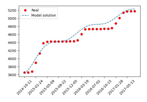
Figure 3: Fitting graph of model solution to real data of laboratory confirmed cases of flu in Nova Scotia, Canada: real data shown as dots and model solution displayed as a dashed line.
5.2. Estimating influenza's basic reproduction number
To approximate the value of the basic reproduction number \(R_0\), we utilize the method described in [3], which involves calculating the largest root of an equation using a continued fraction (see Equation (7)).
Given that the delay used in our numerical simulation for influenza is approximately 0.5 week, which is relatively short compared to the 52-week period of the disease, and consequently \(\beta(t-\Delta)\) is approximately equal to \(\beta(t)\), we approximated \(\beta(t-\Delta)\) with \(\beta(t)\) for simplicity in this subsection.
As discussed in Section 3, the basic reproduction number for the model is given by \(R_0 = r(L_0)\), where:
\[L_0: C_{\omega} \longrightarrow C_{\omega},\]
\[u(t) \longmapsto \int_0^{\infty} k(t, x) u(t - x) dx,\] and
\[\text{[rumus tidak dapat ditampilkan dengan baik — lihat PDF asli]}\] and
\[A(t - \Delta) = e^{-\mu \Delta} (\beta_0 (1 + \epsilon \cos(2\pi t))) (S^* + (1 - \gamma) S_E^*).\]
It follows that \(R_0\) is the largest real such that the equation
\[\int_0^\infty K(t,x)u(t-x)dx = R_0u(t),\]
has an \(\omega\)-periodic solution u(t). For \(n \in \mathbb{N}\) let
\[K_n = \int_0^\infty K(x)e^{-ni2\pi x}dx,\] where
\[K(x) = \begin{cases} 0, & 0 < x < \Delta, \\ e^{-\mu \Delta} \beta_0 (S^* + (1 - \gamma) S_E^*) e^{-(\mu + d)(x - \Delta)}, & x > \Delta. \end{cases}\]
Then
\[K_n = e^{-\mu \Delta} \beta_0 (S^* + (1 - \gamma) S_E^*) \frac{e^{-ni2\pi \Delta}}{\mu + d + ni2\pi}\]
Following the method developed in [3], one can show that \(R_0\) as the largest real root of
\[\frac{R_0}{K_0} - 1 - 2Re \frac{\epsilon^2/4}{\frac{R_0}{K_1} - 1 - \frac{\epsilon^2/4}{\frac{R_0}{K_2} - 1 - \frac{\epsilon^2/4}{W}}} = 0.\] (7)
We limit the continued fraction (7) at the index 1, then we obtain
\[\frac{R_0}{K_0} - 1 - 2Re \frac{\epsilon^2/4}{\frac{R_0}{K_1} - 1} = 0,\] with
\[K_0 = \beta_0 e^{-\mu \Delta} (S^* + (1 - \gamma) S_E^*) \frac{1}{\mu + d},\] and
\[K_1 = \beta_0 e^{-\mu \Delta} (S^* + (1 - \gamma) S_E^*) \frac{e^{i2\pi \Delta}}{\mu + d + i2\pi}.\]
Then we get:
\[\frac{R_0}{K_0} - 1 - \epsilon^2 / 2 \frac{Re(K_1)(R_0 - Re(K_1) - Im(K_1)^2)}{(R_0 - Re(K_1))^2 + Im(K_1)^2} = 0.\]
Using the parameter values as in Table (2), for d=0.015 we have \(R_0\simeq 2.1655\) and for d=0.05 we have \(R_0\simeq 0.52\) and for d=0.026 we get \(R_0\simeq 1\). In the rest of this paper we consider d=0.026 the value for wich \(R_0\) is close to 1.
6. SENSITIVITY ANALYSIS AND PARAMETER IMPACT
6.1. The influence of behavioral changes
In this subsection, we explore the impact of behavior modification on disease spread. Clearly, increasing \(\wedge\) or decreasing \(P^*\) would help in recruiting more individuals into the class \(S_E\). Similarly, increasing \(\gamma\) should aid in reducing the recruitment into the class I of infected individuals. We aim to quantify and compare these expected effects through numerical simulations, assessing each parameter's influence on the disease's dynamics.
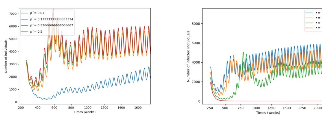
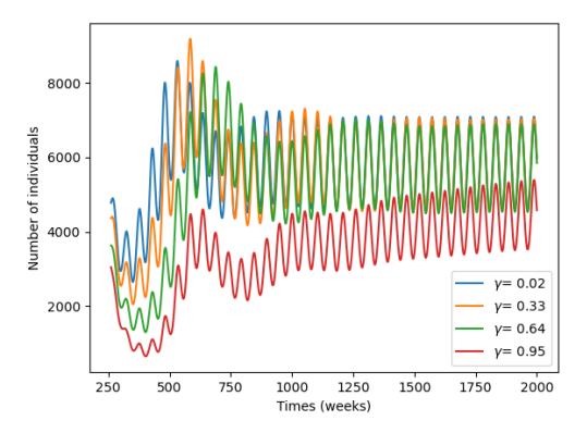
Let us begin by examining how the basic reproduction number, \(R_0\), depends on education-related parameters. At the disease-free equilibrium, where P=0, \(R_0\) does not depend on \(P^*\). Our numerical simulations reveal that \(R_0\) primarily depends on the parameters \(\wedge\) and \(\gamma\). As illustrated in Figure 4, an increase in \(\wedge\) leads to a notable decrease in \(R_0\), an effect that is less pronounced when adjusting \(\gamma\). This may be due to the fitted value of \(\gamma\) being close to 1 (specifically \(\gamma=0.94\)), which could highlight the more significant impact of \(\wedge\). This trend is further confirmed in Figure 5, where we analyze the effects of the parameters \(\gamma\), \(P^*\), and \(\wedge\) on the number of active cases. For this analysis, the value of \(\beta_0\) has been modified to ensure \(R_0>1\), and new solutions have been generated. Figure 5 demonstrates that increasing \(\gamma\) or \(\wedge\) or decreasing \(P^*\) reduces the number of cases, with the impact being more pronounced for \(\wedge\). Even with a \(\gamma\) near 1, or a \(P^*\) near 0, the epidemic persists (see Figure 5b).
To effectively visualize the most notable effects of the parameters \(\land\) and \(P^*\) on disease dynamics, we present a contour plot in Figure 6, which shows the number of cumulative cases after six years as a function of \(P^*\) and \(\land\). The x-axis, showing \(\land\), reveals that a high rate of people moving into the educated class \(S_E\) helps to control the disease: in particular, when \(\land\) is over 100, the cases usually fall below 400. This strong influence is shown by a quick change to cooler colors in the plot, indicating fewer cases. On the other hand, \(P^*\), on the y-axis, doesn't have as strong an impact. Low \(P^*\) values, meaning more people are recruited when the disease is not widespread, don't reduce cases much unless \(\land\) is about 40 or more. Changes in behavior during an epidemic (shown by low \(P^*\)) are helpful, but reducing cases more effectively seems to come from ongoing education (high \(\land\)) rather than reacting to the disease's current state. Therefore, the plot shows that
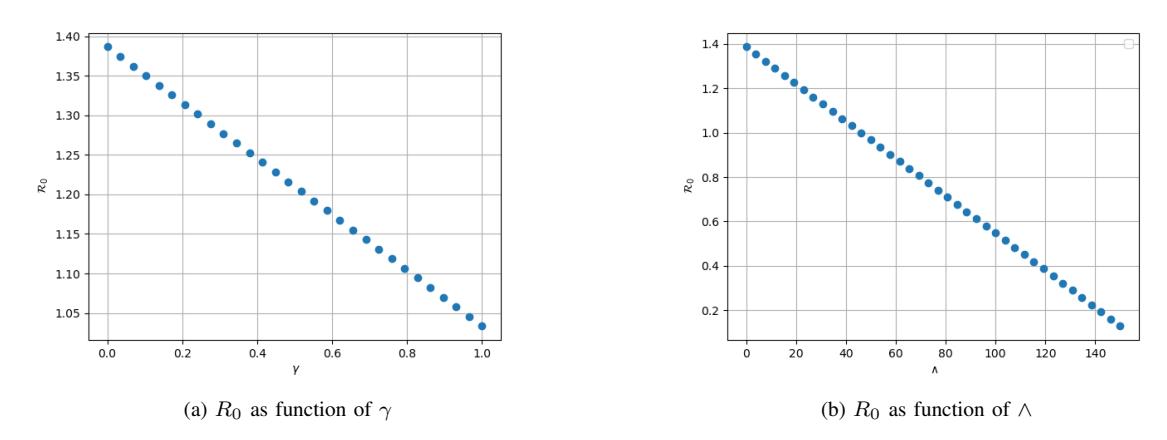
Figure 4: Sensitivity of the basic reproduction number to ∧ and γ, the other parameters are as in Table (2) and d = 0.026.
(a) Number of infected individuals with different values of P

(c) Number of infected individuals with different values of γ
Figure 5: Sensitivity of the number of infected individuals "I" to the parameters ∧, P ∗ and γ with β0 = 1.864 × 10⁻⁶ and the other parameters are as in Table 2.
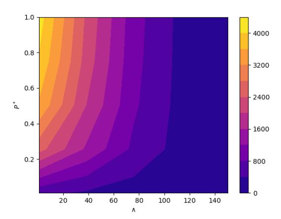
Figure 6: Contour plot representing the number of cases after a period of 6 years as a function of P ∗ and ∧.
continuous education efforts are more effective for long-term disease control than strategies that only react to how much the disease is spreading.
Our model includes two recruitment rates into the compartment SE: a steady recruitment rate (∧) and a rate influenced by the current disease prevalence (P). The numerical simulations reveal that increasing ∧, which signifies proactive and consistent educational efforts, helps to suppress disease propagation and lessens the reliance on reactive measures later when the epidemic is ongoing. This finding is consistent with results in [1], which highlight that delayed interventions by health policymakers often have negligible effects on reducing case numbers. Therefore, our results emphasize the critical need for early and sustained deployment of effective self-protection strategies to foster behavioral change. Early engagement in the educational and sensitising process equips the population to adopt protective measures timely, in the early stage of the epidemic, substantially lowering the potential for disease transmission. In contrast, while P ∗ affects recruitment when prevalence rises, its relative impact is minimal compared to the benefits of early and continuous education provided by ∧, affirming that the latter is a pivotal element in long-term public health strategy.
6.2. Seasonality and incubation: implications for R0
Now we will discuss the effect of seasonality and the latent period on R0. If we assume that all infectious individuals survive during the latency period, i.e., we replace e −µ∆ with 1 in the third equation of (1), we obtain results similar to those presented in [3, Section 4.3]. Figure 7a shows R0 as a function of ∆ in this case. It shows that when ϵ = 0, the basic reproduction number R0 is independent of ∆ and is the same as that for the autonomous epidemic model [11] . It is given by the formula:
\[R_0 = \beta_0 \left( S^* + (1 - \gamma) S_E^* \frac{1}{\mu + d} \right).\] while if ϵ ̸= 0, the basic reproduction number R0 is a 1-periodic function of ∆.
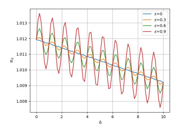
Figure 7b corresponds to the case where e −µ∆ is not replaced with 1 in the third equation of System (1). It shows the basic reproduction number as a function of the latent period ∆ for different values of ϵ, while all other parameters are fixed as previously defined in Table 2. In this case, the basic reproduction number is not a periodic function of ∆. When ϵ = 0, R0 is a decreasing function of ∆ and is given by the formula:
\[R_0 = e^{-\mu \Delta} \beta_0 c \left( S^* + (1 - \gamma) S_E^* \frac{1}{\mu + d} \right).\]
For the case where ϵ ̸= 0, increasing the latent period ∆ tends to decrease R0 not monotonously, but with resonance between ∆ and ω
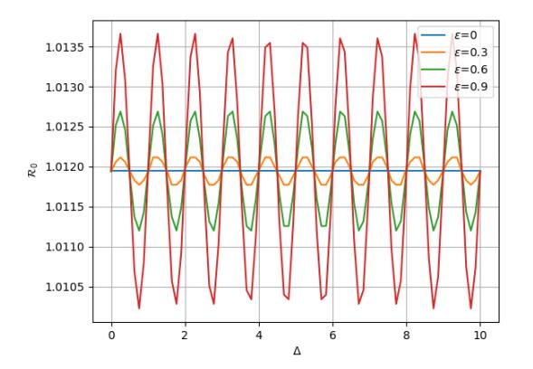
- (a) The case where the infected individuals survive during the latency period. (e−µ∆ replaced with 1 in the third equation of (1)
- (b) The case where infected individuals exhibit a linear growth rate during the latency period (the case of our model (1)).
Figure 7: R0 as a function of ∆ with different values of ϵ, and the other parameter as in Table 2.
7. CONCLUSION
In conclusion, this study introduces a nonlinear model SSEIR where the compartment SE represents susceptible and educated individuals. This model integrates a delay and a periodicity in the incidence rate. Through a sensitivity analysis, we highlighted the impact of various parameters on the basic reproduction number R0. We applied this model to the spread of influenza in Nova Scotia, Canada, and our results highlight the importance of considering self-protection measures in disease modeling. Our study suggests that proactive interventions, including early and ongoing education of individuals in self-protection practices, are more effective in limiting disease transmission than strategies implemented at later stages of the epidemic. However, it is important not to overlook the costs associated with these proactive strategies. Implementing education and awareness measures continuously, even outside of an epidemic, can be expensive and requires careful planning. This paves the way for future research on optimal control strategies to find the right balance between proactive and reactive measures, helping to make better choices in public health responses during outbreaks.