

1. INTRODUCTION
Rumors are widely defined in a variety of studies. However in general, rumors can be understood as unverified information or statements shared by among people that may be positive or negative and they circulate without confirmation [1]. Psychologically, rumors spread because people needs factual information, self enhancement, and social enhancement, as three key motivations in rumor transmission intentions [1], [2]. Consequently, rumors become an inevitable part of human life, including in political aspects, such as elections.
The year 2024 being referred to as "the super or ultimate election year" because more than fifty countries around the world hold elections, with the number of voters potentially representing almost half of the global population [3], [4], [5]. In the context of presidential elections, candidates endeavor to persuade voters through their vision and mission campaigns, while voters based on various considerations endeavor to vote the best candidate. Consequently, terms such as viability, electability, and popularity frequently arise and highlighting the candidates in period leading up to the election.
Research conducted by [6] through two election campaign experiments found that voters engage more extensively with information on viable candidates, rate viable candidates more favorably, and exhibit a higher likelihood of voting. Viability, as perceived by the voter, has previously been conceptually linked to electability in [7] through three proposed voter decision models. This study defined electability as the perceived likelihood of a candidate's success in elections and assumed that assessments of electability are also shaped by voters'
*Corresponding author
Received June 7th, 2024, Revised August 21st, 2024 (first), Revised October 23rd, 2024 (second), Accepted for publication November 15th, 2024. Copyright ©2024 Published by Indonesian Biomathematical Society, e-ISSN: 2549-2896, DOI:10.5614/cbms.2022.7.2.3
opinions of candidates or the candidates' popularity. This is further articulated by [8], [9], who suggests that for many voters, arguments regarding electability are rooted in their own ideological preferences rather than in systematically viewing candidates. Therefore, this contributes to the complexity of the candidate selection process in elections.
Nevertheless, the complexity of electoral process is dynamics because influenced by various aspects that focus on individual candidates and social circumstance [10], [11]. Furthermore, media factor, particularly social media, plays a crucial role in disseminating the rumors [12], [13]. This leads to diverse perceptions within society, causing rumors about candidates to emerge and proliferate more rapidly during the period up to the elections [14], [15]. Therefore, understanding and exploring the dynamics of rumor transmission is both an interesting and important topic of study.
Research on rumor transmission has been a long journey. One of them is by using a mathematical modeling point of view to study the dynamics of rumor transmission. Due to similarity of the spread characteristics between infectious disease and rumors, Daley and Kendall in [16] established the classic mathematical model of rumor transmission. Subsequently, various mathematical models have been proposed and investigated. Some studies utilize compartmental models that account for people's varying mechanism or attitudes toward rumors [17], [18], [28]. Other studies focus on compartmental models within multilingual environment, incorporating media reports about rumors [19], [20]. Additionally, prior study has developed a stochastic model to examine the relationship between user following and the impact level of rumors on social media [21]. This study revealed that a higher number of followers contributed to a decrease in the spread of rumors from a spesific following. A recent study conducted by Huang et al. in [22] proposed a multiplex network model to analyze the competitive diffusion of knowledge and rumor. This study highlighted the importance of reinforcing and integrating knowledge among rumor spreaders and listeners. Furthermore, another recent study conducted by Chen and Srivastava in [23] proposed a rumor propagation model with spatial heterogeneity.
Although the above research thoroughly explores the dynamics of rumor transmission, studies focusing on rumor dynamics in the context of elections are rarely conducted, particularly from a mathematical perspective. Most prior research have analyzed rumors from political and socio-psychological viewpoints [24], [25], [26]. However, mathematics offers a promising approach to better understand the dynamics of rumor spread over a certain period [27]. Additionally, we observed that some prior studies provided numerical simulations based on assumed model parameter values.
Motivated by the background, prior research, and these considerations, this study constructs a mathematical model to explore the dynamics of rumor spread within the context of an electoral process. The model is adapted from [28], incoporating people's different attitudes toward rumors about two candidates. The mechanism of rumor transmission and its parameters were designed to align as closely as possible with the actual conditions, using the 2008 U.S. Presidential election as a case study based on an immersive literature review. We provide analytical review of model, supported by numerical experiments and simulations to enhance accessibility. Finally, this study offers valuable insights into the dynamics of rumor spread and its relationship with public attitudes in an electoral setting as a conclusion. Therefore, this study aims to obtain an in-depth understanding of how rumors spread in society during the electoral process.
The rest of this paper is organized as follows. In section (2), we formulate the model of rumor spread dynamics, describe the variables and parameters used in the model, and prove its positivity and boundedness. In section (3), we examine the model's dynamic behavior by deriving the rumor free equilibrium and basic reproductive number, and the rumor existence equilibrium; we also provide numerical experiments to verify the stability of these equilibrium, followed by a sensitivity analysis of the basic reproductive number with respect to the model parameters. In section (4), we present numerical simulations of the model. Finally, in section (5), we provide concluding remarks.
2. MODEL FORMULATION
The mathematical model of rumor spread dynamics in the election is first constructed by dividing the total population, N(t), into five subpopulations represented as compartment groups. These compartments include the different attitudes of people when exposed to rumors: susceptible people (S), hesitant people (H), affected people for candidate 1 rumors (I1), affected people for candidate 2 rumors (I2), and resistant people to rumors (R). We assume that the total population remains constant and comprising eligible and registered voters. Additionally, we assume that rumors spread directly within the population or human to human transmission. It is important to note that media plays a supporting role in the rumor transmission, regardless its validity [29].
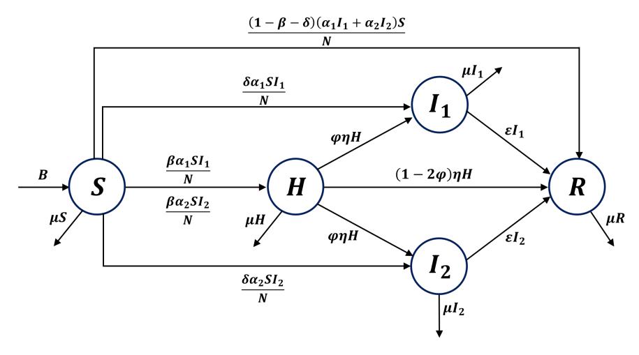
Figure 1: Compartmental diagram of the rumor spread model in the election context. Note that S compartment have the possibility to move directly into any of the other four compartments.
Table 1: Description of variables and parameters in the model (1)
| Notation | Description |
|---|---|
| S(t) | Number of susceptible people who have not heard any rumors about candidates at time \(t\) |
| H(t) | Number of hesitated people who have heard any rumors about candidates at time \(t\) |
| \(I_1(t)\) | Number of affected people who are affected by rumors of candidate 1 and spread the rumor at time \(t\) |
| \(I_2(t)\) | Number of affected people who are affected by rumors of candidate 2 and spread the rumor at time \(t\) |
| R(t) | Number of resistant people who disbelief any rumors and do not spread the rumor at time \(t\) |
| B | Rate of people entering the population \(\left(\frac{\text{people}}{\text{day}}\right)\) |
| \(\alpha_1\) | Rate of rumor transmission about candidate \(1\left(\frac{1}{day}\right)\) |
| \(\alpha_2\) | Rate of rumor transmission about candidate 2 \((\frac{\vec{a}}{day})\) |
| \(\eta\) | Rate of progression from hesitated to affected or resistant people \((\frac{1}{day})\) |
| \(\varepsilon\) | Rate of affected people become resistant people \((\frac{1}{day})\) |
| \(\beta\) | Proportion of susceptible people become hesitated people |
| \(\delta\) | Proportion of susceptible people become affected people |
| \(\varphi\) | Proportion of hesitated people become affected people |
| \(\mu\) | Rate of people who have leaving out the population \(\left(\frac{1}{\text{day}}\right)\) |
In this study, we focus on the case involving two candidates, candidate 1 and candidate 2, with initial equal electability as assumption. The number of people entering the population per unit of time consists of people who have not yet heard any rumors about the two candidates, with a recruitment rate denoted as B. These subpopulation are considered susceptible people and belong to the S compartment. During the period up to the election, susceptible people hear rumors about candidate 1 and candidate 2 through contact with others person, with transmission rates \(\alpha_1\) and \(\alpha_2\), respectively. People who immediately become affected by the rumors of candidate 1 or candidate 2 with proportion of \(\delta\), will belong to the \(I_1\) or \(I_2\) compartments, represented by \(\frac{\delta \alpha_1 S I_1}{N}\) or \(\frac{\delta \alpha_2 S I_2}{N}\), respectively.
In reality, not everyone immediately believes the rumors regarding the two candidates. The phenomenon of undecided and swing voters could be a reason that people who have heard rumors potentially become hesitant [30], [31]. Hence, some people may become hesitant with proportion of \(\beta\) when they hear rumors. This subpopulation is hesitating people and belong to the H compartment as \(\frac{\beta\alpha_1SI_1}{N}\) or \(\frac{\beta\alpha_2SI_2}{N}\). After some consideration, this population may decrease as they change their attitudes at a rate of progression \(\eta\). When hesitant people decide to believe and spread the rumors about the two candidates with proportion of \(\varphi\), they belong to the \(I_1\) and \(I_2\) compartments respectively as \(\varphi\eta H\). Conversely, when hesitant people decide to disbelieve and refrain from spreading rumors at the same rate of progression \(\eta\), they belong to R compartment, represented as \((1-2\varphi)\eta H\).
Furthermore, the affected people in \(I_1\) and \(I_2\) compartments may decrease because they still have the possibility to change their attitudes and become disbelievers of the rumors about the two candidates at a rate of \(\varepsilon\). People decided not to spread the rumors, become resistant people, and belong to the R compartment as \(\varepsilon I_1\) or \(\varepsilon I_2\). Additionally, the R compartment can also increase if susceptible people in the S compartment, who are neither hesitated nor affected by the rumors of two candidates, immediately decide to resist the rumors. This is represented by \(\frac{(1-\beta-\delta)(\alpha_1 I_1+\alpha_2 I_2)S}{N}\). We assume that resistant people will not potentially return to being susceptible people.
All compartments may also decrease due to people leave out the population for some reasons at a rate of \(\mu\). All rates and proportions are positive constant, with the proportion of \(\beta\), \(\delta\), and \(\varphi\) satisfying the conditions \(\beta + \delta < 1\) and \(\varphi < 0.5\). The total population is given by \(N(t) = S(t) + H(t) + I_1(t) + I_2(t) + R(t)\).
Based on the assumptions and descriptions provided above, we can visualize a compartmental diagram of the rumor spread, as shown in Figure (1). The mathematical model of rumor spread dynamics in the election can be formulated into a system of differential equation in Model (1). Detailed description of variables and parameters used in this model can be seen in Table 1.
\[\frac{dS}{dt} = B - \frac{\alpha_1 S I_1}{N} - \frac{\alpha_2 S I_2}{N} - \mu S,\] \[\frac{dH}{dt} = \frac{\beta \alpha_1 S I_1}{N} + \frac{\beta \alpha_2 S I_2}{N} - \eta H - \mu H,\] \[\frac{dI_1}{dt} = \frac{\delta \alpha_1 S I_1}{N} + \varphi \eta H - \varepsilon I_1 - \mu I_1,\] \[\frac{dI_2}{dt} = \frac{\delta \alpha_2 S I_2}{N} + \varphi \eta H - \varepsilon I_2 - \mu I_2,\] \[\frac{dR}{dt} = \frac{(1 - \beta - \delta)(\alpha_1 I_1 + \alpha_2 I_2)S}{N} + (1 - 2\varphi)\eta H + \varepsilon I_1 + \varepsilon I_2 - \mu R.\] (1)
2.1. Positivity and boundedness of the model
To show the model of rumor dynamics is biologically and contextually meaningful, we will prove that all solutions of Model (1) are positive and bounded for all time t > 0.
Theorem 2.1. All the solutions of Model (1), i.e. S(t), H(t), \(I_1(t)\), \(I_2(t)\), and R(t), are always positive for t > 0 with the initial condition S(0) > 0, \(H(0) \ge 0\), \(I_1(0) \ge 0\), \(I_2(0) \ge 0\), and \(R(0) \ge 0\).
Proof: From the first equation of Model (1), we obtain
\[\frac{dS}{dt} + \left(\frac{\alpha_1 I_1}{N} + \frac{\alpha_2 I_2}{N} + \mu\right) S = B. \tag{2}\]
Define the integration factor: \(C(t) = \exp\left(\int_0^T \mathcal{M} \, dt\right)\), with \(\mathcal{M} = \left(\frac{\alpha_1 I_1}{N} + \frac{\alpha_2 I_2}{N} + \mu\right)\).
By multiplying equation (2) with C(t), we obtain
\[\frac{dS}{dt} \exp\left(\int_0^T \mathcal{M} dt\right) + \mathcal{M}S \exp\left(\int_0^T \mathcal{M} dt\right) = B \exp\left(\int_0^T \mathcal{M} dt\right),\] then write it into
\[\frac{d}{dt}\left(S\exp\left(\int_0^T \mathcal{M}\,dt\right)\right) = B\exp\left(\int_0^T \mathcal{M}\,dt\right). \tag{3}\]
Furthermore, by integrating the both parts of equation (3), we obtain
\[S(T) = \exp\left(-\int_0^T \mathcal{M} \, dt\right) \left[S(0) + \int_0^T B \exp\left(\int_0^T \mathcal{M} \, dt\right)\right] > 0.\]
With a similar process, it can be obtained that H(T), \(I_1(T)\), \(I_2(T)\), R(T) > 0. Therefore, we can conclude that all the solutions of Model (1) are always positive as long as the initial condition are non-negative. The proof is completed.
Theorem 2.2. All the subpopulations of Model (1), i.e. S(t), H(t), \(I_1(t)\), \(I_2(t)\), and R(t), are bounded.
Proof: Consider that the total of human population is \(N = S + H + I_1 + I_2 + R\), then by adding up all the equation in Model (1), we obtain
\[\frac{dN}{dt} = B - \mu N. \tag{4}\]
Furthermore, suppose that \(N(0) = N_0\). By solving equation (4), we obtained the solution
\[N(t) = \frac{B}{\mu} + \left(N_0 - \frac{B}{\mu}\right)e^{-\mu t}.\] (5)
For \(t \to \infty\), we obtained
\[\lim_{t \to \infty} N(t) = \frac{B}{\mu},\]
thus \(N(t) \leq \frac{B}{\mu}\). Therefore, based on theorem (2.1), we obtained that all solutions of Model (1), i.e. S(t), H(t), \(I_1(t)\), \(I_2(t)\), and R(t), are bounded in \(\left[0, \frac{B}{\mu}\right]\). The proof is completed.
\[H(t), I_1(t), I_2(t),\] and \(R(t)\), are bounded in \(\left[0, \frac{B}{\mu}\right]\). The proof is completed.
Based on theorem (2.1) and (2.2), we can conclude that Model (1) satisfies the positive invariant region as summarized in the following corollary.
Corollary 2.2.1. Region \(\Omega = \left\{ (S, H, I_1, I_2, R) \in \mathbb{R}^5_+ | N = S + H + I_1 + I_2 + R \leq \frac{B}{\mu} \right\}\) is positively invariant for Model (1) with initial conditions S(0) > 0, \(H(0) \ge 0\), \(I_1(0) \ge 0\), \(I_2(0) \ge 0\), and \(R(0) \ge 0\).
Furthermore, since the R compartment does not appear in the other compartments, Model (1) can be simplified into Model (6) as follows
\[\frac{dS}{dt} = B - \frac{\alpha_1 S I_1}{N} - \frac{\alpha_2 S I_2}{N} - \mu S, \frac{dH}{dt} = \frac{\beta \alpha_1 S I_1}{N} + \frac{\beta \alpha_2 S I_2}{N} - \eta H - \mu H, \frac{dI_1}{dt} = \frac{\delta \alpha_1 S I_1}{N} + \varphi \eta H - \varepsilon I_1 - \mu I_1, \frac{dI_2}{dt} = \frac{\delta \alpha_2 S I_2}{N} + \varphi \eta H - \varepsilon I_2 - \mu I_2.\] (6)
This model will analyze in the following section, instead of the original model (1), without compromising the overall dynamics of the model.
3. MODEL ANALYSIS
3.1. Rumor free equilibrium and basic reproductive number
Rumor free equilibrium (RFE) is a condition where there are no rumors at all in the society regarding candidate 1 and candidate 2. Based on Model (6), this condition occurs when \(H(t) = I_1(t) = I_2(t) = 0\), so the following result are obtained
\[\frac{dS}{dt} = B - \mu S \Longleftrightarrow S(t) = \frac{B}{\mu}.\]
Therefore, we obtained the rumor free equilibrium as follows
\[RFE = (S, H, I_1, I_2) = \left(\frac{B}{\mu}, 0, 0, 0\right).\] (7)
Furthermore, the basic reproductive number \((\mathcal{R}_0)\) of Model (6) will be determined by adapting the Next-Generation Matrix (NGM) Method, which has been developed by several researchers [32], [33]. In this case, \(\mathcal{R}_0\) is defined as the average number of new individuals affected and potentially becoming the rumor spreaders due to an individual entering and spreading rumors, either related to candidate 1 or candidate 2, in the susceptible population. Consider the transmission compartments of Model (6), suppose \(X = [H I_1 I_2]^T\). Model (6) can be written as follows
\[\frac{dX}{dt} = \mathcal{F}(X) - \mathcal{V}(X),\]
with
\[\mathcal{F}(X) = \begin{bmatrix} \frac{\beta \alpha_1 S I_1}{N} + \frac{\beta \alpha_2 S I_2}{N} \\ \frac{\delta \alpha_1 S I_1}{N} \\ \frac{\delta \alpha_2 S I_2}{N} \end{bmatrix}\](8)
and
\[\mathcal{V}(X) = \begin{bmatrix} \eta H + \mu H \\ \mu I_1 + \varepsilon I_1 - \varphi \eta H \\ \mu I_2 + \varepsilon I_2 - \varphi \eta H \end{bmatrix}. \tag{9}\]
Evaluate (8) and (9) at the RFE, then we obtained the transmission matrix
\[F = \begin{bmatrix} 0 & \frac{\beta\alpha_1 B}{\mu N} & \frac{\beta\alpha_2 B}{\mu N} \\ 0 & \frac{\delta\alpha_1 B}{\mu N} & 0 \\ 0 & 0 & \frac{\delta\alpha_2 B}{\mu N} \end{bmatrix}\](10)
and the transition matrix
\[V = \begin{bmatrix} \eta + \mu & 0 & 0 \\ -\varphi \eta & \mu + \varepsilon & 0 \\ -\varphi \eta & 0 & \mu + \varepsilon \end{bmatrix}.\] (11)
Based on matrix (10) and (11), we obtain the basic reproductive number of Model (6) by determine the spectral radius of the next-generation matrix, as follows
\[\mathcal{R}_0 = \rho(FV^{-1}) = \frac{(\alpha_1 + \alpha_2)(\eta + \mu)\delta B + (\alpha_1 + \alpha_2)\beta\varphi\eta B + B\sqrt{\Delta}}{2(\eta + \mu)(\varepsilon + \mu)\mu N},\] (12)
where \(\Delta = (\alpha_1 + \alpha_2)^2 (\beta \varphi \eta)^2 + (\alpha_1 - \alpha_2)^2 (\eta + \mu)(2\beta \eta \mu + \delta \eta + \delta \mu)\delta\).
To determine the stability of RFE, we linearize Model (6) and evaluate it at RFE point in (7). Thus, we obtained the Jacobian matrix in RFE as follows
\[J(RFE) = \begin{bmatrix} -\mu & 0 & -\alpha_1 \frac{B}{\mu N} & -\alpha_2 \frac{B}{\mu N} \\ 0 & -\eta - \mu & \alpha_1 \beta \frac{B}{\mu N} & \alpha_2 \beta \frac{B}{\mu N} \\ 0 & \varphi \eta & \alpha_1 \delta \frac{B}{\mu N} - \varepsilon - \mu & 0 \\ 0 & \varphi \eta & 0 & \alpha_2 \delta \frac{B}{\mu N} - \varepsilon - \mu \end{bmatrix}.\] (13)
The characteristic polynomial of J(RFE) is
\[(\lambda + \mu)(\lambda^3 + p_2\lambda^2 + p_1\lambda + p_0) = 0, (14)\]
where
\[p_{2} = 3\mu + 2\varepsilon + \eta - (\alpha_{1} + \alpha_{2})\delta \frac{B}{\mu N},\] \[p_{1} = (\mu + \varepsilon)2\eta + (3\mu + \varepsilon)(\mu + \varepsilon) + \alpha_{1}\alpha_{2}\delta^{2}\left(\frac{B}{\mu N}\right)^{2} - (\alpha_{1} + \alpha_{2})\left(2\delta B + \beta\eta\varphi \frac{B}{\mu N} + \delta\varepsilon \frac{B}{\mu N} + \delta\eta \frac{B}{\mu N}\right),\] \[p_{0} = (\mu + \eta)(\mu + \varepsilon)^{2} + \alpha_{1}\alpha_{2}\delta^{2}\frac{B^{2}}{\mu N} + \alpha_{1}\alpha_{2}\eta(\delta^{2} + 2\beta\delta\varphi)\left(\frac{B}{\mu N}\right)^{2} - (\alpha_{1} + \alpha_{2})(\beta\varepsilon\eta\mu + \delta\varepsilon\eta)\frac{B}{\mu N}\] \[- (\alpha_{1} + \alpha_{2})(\delta\mu B + \delta\varepsilon B + \delta\eta B + \beta\eta\varphi B).\]
We have obtained one root of the characteristic polynomial in equation (14), that is \(\lambda_1 = -\mu\). Due to the complexity of the other characteristic polynomial roots, we performed numerical experiments for stability of rumor free equilibrium in section (3.3).
3.2. Rumor existence equilibrium
In the human society development, especially in the context of elections, rumors will always circulate in society related to the candidates [23]. Rumor existence equilibrium (REE) is a condition where rumors will always circulate in society regarding the two candidates. The REE of Model (6) is \((S^*, H^*, I_1^*, I_2^*)\) and obtained by solving the model at steady state condition, that is when \(\frac{dS}{dt} = 0\), \(\frac{dH}{dt} = 0\), \(\frac{dI_1}{dt} = 0\), and \(\frac{dI_2}{dt} = 0\). By solving it, we obtained the REE of Model (6) for \(S^*\) and \(H^*\), are given by
\[S^* = \frac{BN}{\alpha_1 I_1 + \alpha_2 I_2 + \mu N}, H^* = \frac{\beta B(\alpha_1 I_1 + \alpha_2 I_2)}{(\eta + \mu)(\alpha_1 I_1 + \alpha_2 I_2 + \mu N)}.\]
On the contrary, \(I_1^*\) and \(I_2^*\) is considered by solving the quadratic equations as follows
\[f(I_1) = a_2 I_1^2 + a_1 I_1 + a_0 (15)\]
and
\[g(I_2) = b_2 I_2^2 + b_1 I_2 + b_0, (16)\]
with
\[\begin{split} a_2 &= (\varepsilon + \mu)(\eta + \mu)\alpha_1, \\ a_1 &= (\varepsilon + \mu)(\eta + \mu)(\alpha_2 I_2 + \mu N) - (\eta + \mu)\delta\alpha_1 B - \varphi \eta \beta \alpha_1 B, \\ a_0 &= -\varphi \eta \beta \alpha_2 I_2 B, \\ b_2 &= (\varepsilon + \mu)(\eta + \mu)\alpha_2, \\ b_1 &= (\varepsilon + \mu)(\eta + \mu)(\alpha_1 I_1 + \mu N) - (\eta + \mu)\delta\alpha_2 B - \varphi \eta \beta \alpha_2 B, \\ b_0 &= -\varphi \eta \beta \alpha_1 I_1 B. \end{split}\]
Since \(a_2 > 0\), \(b_2 > 0\) and \(a_0 < 0\), \(b_0 < 0\), then equation (15) and (16) are assured to have one single positive solution. Therefore, \(I_1^*\) and \(I_2^*\) are obtained by taking \(I_1 > 0\) and \(I_2 > 0\).
Consider that \(S^*\) and \(H^*\) include both \(I_1\) and \(I_2\), while \(I_1\) depends on \(I_2\) and vice versa. Based on these considerations, we can reasonably interpret that all subpopulation in Model (6) depend on the number of affected people during the election period. Additionally, a candidate who are not elected does not imply they received no votes. Therefore, with respect to the rumors, we assume that the possible conditions for \(I_1^*\) and \(I_2^*\) are \(I_1^* > I_2^*\) or \(I_2^* < I_1^*\), with \(I_1^* \neq 0\) and \(I_2^* \neq 0\). To analyze the stability of the rumor existence equilibrium in Model (6), we performed numerical experiments as discussed in section (3.3).
3.3. Numerical experiment
To perform numerical experiments on the stability of the rumor free and rumor existence equilibrium, we use the parameter values provided in Table (2). These set of parameter values are based on several literature studies of the 2008 U.S. Presidential election, with the assumption that the transmission rate of candidate 1 is higher than candidate 2.
| Parameter | Value | Reference | Parameter | Value | Reference |
|---|---|---|---|---|---|
| \(\alpha_1\) | 2.0905 | Estimated | \(\delta\) | 0.72 | [35] |
| \(\alpha_2\) | 1.2898 | Estimated | \(\varphi\) | 0.04 | Assumption |
| \(\mu\) | 0.088 | [34] | \(\eta\) | 0.23 | [35] |
| β | 0.22 | [35] | \(\varepsilon\) | 0.312 | [35] |
| N | 146311 | [34] | B | \(N \times \mu\) | Assumption |
Table 2: Baseline parameter values for the rumor dynamics model.
Firstly, for the rumor free equilibrium, we use all the parameter values in Table (2), except \(\alpha_1 = 0.5\) and \(\alpha_2 = 0.3\), that result in \(\mathcal{R}_0 = 0.91 < 1\). The rumor free equilibrium of Model (6) obtained as follows
\[RFE = (S, H, I_1, I_2) = \left(\frac{B}{\mu}, 0, 0, 0\right) = (146311, 0, 0, 0).\] (17)
By evaluating the Jacobian matrix at the RFE in (17) with the baseline parameter values in Table (2), we obtains
\[J(RFE) = \begin{bmatrix} -0.088 & 0 & -0.5 & -0.3 \\ 0 & -0.318 & 0.11 & 0.066 \\ 0 & 0.0092 & -0.04 & 0 \\ 0 & 0.0092 & 0 & -0.184. \end{bmatrix}.\](18)
The eigenvalues of J(RFE) in (18) are
\[\lambda_1 = -0.088, \ \lambda_2 = -0.326, \ \lambda_3 = -0.036, \ \lambda_4 = -0.179.\]
Since all the eigenvalues are negative, we can conclude that RFE is locally asymptotically stable for a set of parameters such that \(\mathcal{R}_0 < 1\).
Secondly, we use all the parameter values in Table (2) including \(\alpha_1\) and \(\alpha_2\) that gives \(\mathcal{R}_0 = 3.804 > 1\). By evaluating the Jacobian matrix at the RFE in (17) with the baseline parameter values in Table (2), we obtains
\[J(RFE) = \begin{bmatrix} -0.088 & 0 & -2.09 & -1.29 \\ 0 & -0.318 & 0.46 & 0.284 \\ 0 & 0.0092 & 1.11 & 0 \\ 0 & 0.0092 & 0 & -0.529. \end{bmatrix}.\] (19)
The eigenvalues of J(RFE) in (19) are
\[\lambda_1 = -0.088, \ \lambda_2 = -0.309, \ \lambda_3 = -0.54, \ \lambda_4 = 1.113.\]
Since \(\lambda_4 > 0\), we conclude that the rumor free equilibrium of Model (6) in (17) is unstable.
Furthermore, due to the complexity of the analytical form of the rumor existence equilibrium in Model (6), we subtitute all the parameter values in Table (2). As a result, the system of equations for Model (6) can be expressed as follows
\[\frac{dS}{dt} = 12875 - (1.4 \times 10^{-5})SI_1 - (8.8 \times 10^{-6})SI_2 - 0.088S, \frac{dH}{dt} = (3.1 \times 10^{-6})SI_1 + (1.9 \times 10^{-6})SI_2 - 0.318H, \frac{dI_1}{dt} = (1.02 \times 10^{-5})SI_1 + 0.0092H - 0.4I_1, \frac{dI_2}{dt} = (6.3 \times 10^{-6})SI_2 + 0.0092H - 0.4I_2.\] (20)
We solve the system of equations in (20) considering all the variables at steady state condition. The rumor existence equilibrium is obtained as follows
\[REE = (S^*, H^*, I_1^*, I_2^*) = (39639, 6533, 16663, 400).\] (21)
By linearizing the system of equations in (20) on the respected REE in (21), we obtained the Jacobian matrix at REE as follows
\[J(REE) = \begin{bmatrix} -0.088 & 0 & -3.69 \times 10^{-6} & -2.32 \times 10^{-6} \\ 3.84 \times 10^{-8} & -0.318 & 8.16 \times 10^{-7} & 5 \times 10^{-7} \\ 1.22 \times 10^{-7} & 0.0092 & -0.399 & 0 \\ 1.89 \times 10^{-9} & 0.0092 & 0 & -0.399. \end{bmatrix}.\] (22)
The eigenvalues of J(REE) in (22) are
\[\lambda_1 = -0.088, \ \lambda_2 = -0.318, \ \lambda_3 = -0.399, \ \lambda_4 = -0.399.\]
Since all the eigenvalues are negative, we can conclude that the rumor existence equilibrium in (21) is locally asymptotically stable for a set parameters in Table (2) such that \(\mathcal{R}_0 > 1\).
3.4. Sensitivity analysis
To analyze the role of parameters in the rumor spread, sensitivity analysis is conducted to qualitatively determine the parameters that most influence in \(\mathcal{R}_0\) or Model (6). We perform the local sensitivity analysis with the following definition.
Definition 1. [36] The local (normalized) sensitivity index of quantity Q with respect to a given parameter p is defined by
\[\Gamma_Q^p = \frac{\partial Q}{\partial p} \times \frac{p}{Q}.\]
Implemented the definition above, we have the sensitivity of \(\mathcal{R}_0\) respect to \(\alpha_1\) form, as follows
\[\Gamma_{\mathcal{R}_{0}}^{\alpha_{1}} = \frac{\partial \mathcal{R}_{0}}{\partial \alpha_{1}} \times \frac{\alpha_{1}}{\mathcal{R}_{0}}\] \[= \frac{\alpha_{1} \varphi \eta B + ((\alpha_{1} + \alpha_{2})(\beta \eta \mu)^{2} + (\alpha_{1} - \alpha_{2})(\eta + \mu)(2\beta \eta \mu + \delta \eta + \delta \mu)\delta) \alpha_{1} B \sqrt{\Delta}}{2\eta \mu^{2} (\varepsilon + \mu) \mathcal{R}_{0}}.\] (23)
Considering the case of \(\alpha_1 > \alpha_2\), we observe that \(\Gamma_{\mathcal{R}_0}^{\alpha_1} > 0\). Therefore, we can conclude that increasing \(\alpha_1\) will increase the \(\mathcal{R}_0\). Furthermore, by subtituting all the parameter values in Table (2) to the \(\Gamma_{\mathcal{R}_0}^{\alpha_1}\) form in (23), we obtained that \(\Gamma_{\mathcal{R}_0}^{\alpha_1} = 0.1872\). Therefore, we can also conclude that increasing the rate of rumor transmission about candidate 1 for 10% will increase the \(\mathcal{R}_0\) for 1.872%. With similarly process, the complete results for the sensitivity of \(\mathcal{R}_0\) respect to all the parameters are shown in Table (3).
Based on Table (3), we observed that all the parameters in \(\mathcal{R}_0\) have the positive sensitivity index, except \(\alpha_2\) and \(\mu\). We have \(\Gamma_{\mathcal{R}_0}^{\alpha_2} = -0.1134 < 0\) which can be conclude that increasing \(\alpha_2\) will reduce \(\mathcal{R}_0\). This
| Parameter (p) | \(\Gamma^p_{\mathcal{R}_0}\) | Parameter (p) | \(\Gamma^p_{\mathcal{R}_0}\) |
|---|---|---|---|
| \(\alpha_1\) | 0.1872 | δ | 0.996 |
| \(\alpha_2\) | -0.1134 | \(\varphi\) | 0.0027 |
| \(\mu\) | -0.9794 | \(\eta\) | 0.0545 |
| \(\beta\) | 0.004 | \(\varepsilon\) | 0 |
| B | 1 |
Table 3: Sensitivity index of \(\mathcal{R}_0\) considering all the parameters in Model (6).
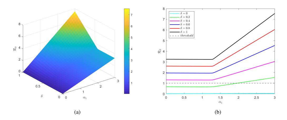
Figure 2: Level set of \(\mathcal{R}_0\) with respect to \(\alpha_1\) and \(\delta\).
means, increasing the rate of rumor transmission about candidate 2 for 10% will reduce \(\mathcal{R}_0\) for 1.134%. In addition, we have \(\Gamma^{\mu}_{\mathcal{R}_0} = -0.9794\) which can be concluded that increasing the rate of people who left out the population for 10% will reduce \(\mathcal{R}_0\) for 9.794%.
Considering the sensitivity analysis in Table (3), we observed that B, \(\mu\), and \(\delta\) are the most influential parameter in \(\mathcal{R}_0\). However, since B and \(\mu\) are naturally interrelated, we focus on \(\delta\) as the most influential parameter that can reasonably considered in an electoral context. Therefore, since \(\Gamma^{\delta}_{\mathcal{R}_0} = 0.996 > 0\), the race to increase \(\alpha_1\) and \(\alpha_2\) in society should be oriented to increasing \(\delta\). Based on this analysis, we interpret that the popularity dynamics of candidates as a consequence of rumor are primarily determined by the number of susceptible people who change become affected people directly. Consequently, the number of rumor spreaders will increase, ensuring that rumors continue to circulate in society, at least throughout the election period.
Subsequently, to visually analyze how the dynamics of \(\mathcal{R}_0\) vary with respect to key parameters, particularly \(\delta\), \(\alpha_1\), and \(\alpha_2\), we present the level set of \(\mathcal{R}_0\) with respect to these parameters. The level set is obtained by evaluating the \(\mathcal{R}_0\) expression using the parameter values outlined in Table (2), and let the parameter observation as independent. For instance, we analyze the influence of \(\alpha_1\) and \(\delta\) on \(\mathcal{R}_0\). Let \(\alpha_1\) and \(\delta\) be free parameters, we can obtain the function of \(\mathcal{R}_0\), as follows
\[\mathcal{R}_{0}\left(\alpha_{1},\delta\right)=\frac{\left(\alpha_{1}+1.2898\right)4094.25\,\delta+12875\sqrt{\left(\alpha_{1}+1.2898\right)^{2}4.1\times10^{-6}+\left(\alpha_{1}-1.2898\right)^{2}0.0757\,\delta}}{\left(2.24\times10^{-2}\right)146311}\] and the level set of \(\mathcal{R}_0\) respect to \(\alpha_1\) and \(\delta\) is shown in Figure (2).
Based on Figure 2(a), it can be observed that increasing \(\alpha_1\) and \(\delta\) simultaneously will result in an increase \(\mathcal{R}_0\). While, the dependency of \(\alpha_1\) considering various values of \(\delta\) is shown in Figure 2(b). Based on these figure, we can observe that increasing \(\delta\) necessary the condition \(\alpha_1 > \alpha_2\) such that \(\mathcal{R}_0 > 1\). This condition
will make R0 > 1 occurs more rapidly. If in any condition, δ value turns out to be quite small, for instance δ = 0.2 as shown in Figure 2(b), the R0 can still increase and exceed one as long as α1 continues to increase beyond α2. Furthermore, If the condition is α1 < α2, a much higher value of δ is required for R0 > 1 to be achieved. Therefore, a necessary and sufficient condition for the rumors of a candidate continue circulating in society is an increase in the proportion of people who change from susceptible to affected, followed by a rumor transmission rate higher than the opposing candidate. In the context of elections, this analysis can be interpreted as a candidate's campaign strategy with the main objective of convincing voters to support them.
4. SIMULATION
In this section, we present some numerical simulations of the proposed rumor model in (1). The simulations aim to explore the dynamics of the model compartments or subpopulations and their relation to changes in some parameter values. As a case study, we used the popularity of two candidates in 2008 U.S. Presidential election, based on popularity dynamics in Google Trends during an observation period of 40 days before election day [37] with thoroughly considerations. Using the popularity data of these two candidates, we estimated the parameter values of α1 and α2 by employing the nonlinear least square solver available in Matlab. The objective was to minimize the sum of squared distance between the data and the model dynamics for the I1 and I2 compartments using the best-fit parameters of α1 and α2.
To conduct the simulations, we used the model parameter values as shown in Table (2), with the exception of α1, α2 and δ, which were varied in some simulations. The total population used in the simulations is N = 146311, representing the total number of registered voters in the 2008 U.S. Presidential election [34]. Therefore, the initial population values are set as S(0) = 146000, H(0) = 0, I1(0) = 155, I2(0) = 156, and R(0) = 0 for the model simulations.
Firstly, we performed simulations to verify the numerical experiment results from the previous section regarding the stability of rumor free and rumor existence equilibrium. We used the same transmission rates, α1 = 0.5 and α2 = 0.3, which result in R0 = 0.91. The simulation of the rumor dynamics is shown in Figure 3(a). This simulation confirms that when R0 < 1, rumors cannot spread in society. This is indicated by the absence of changes in the dynamics of the hesitated, affected, and resistant subpopulations, while susceptible people remains constant at its equilibrium value.
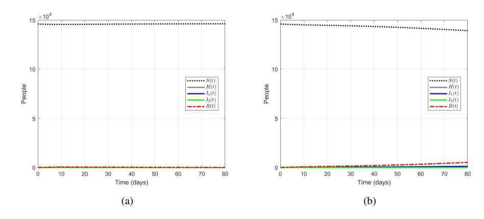
Figure 3: Simulation of rumor spread dynamics for: (a) α1 = 0.5 and α2 = 0.3 that gives R0 < 1, (b) α1 = 0.6 and α2 = 0.4 that gives R0 > 1.
Furthermore, to simulate the stability of the rumor existence equilibrium, we used α1 = 0.6 and α2 = 0.4, which gives R0 close to one, spesifically R0 = 1.092. The simulation of the rumor dynamics is shown in Figure 3(b). We observe changes in dynamics, particularly an increase in the number of resistant people and a decrease in the susceptible people. This indicates that rumors are spreading in society, even though quite slowly. Therefore, these simulation results confirm that when R0 > 1, rumors will circulate in the society and tend to be stable at a certain time.
Secondly, we performed the main simulations of the rumor dynamics in Model (1), as shown in Figure (4) and (5). The transmission rates of the rumor were based on the values of α1 and α2 listed in Table (2). In accordance with the numerical experiments from the previous section, the input parameters yields R0 = 3.804 > 1, indicating the rumor will continue to circulate and remain stable in society. This is further confirmed in Figure (4), where the number of resistant people consistently exceeds that of the other subpopulations, at least after seven days. Meanwhile, Figure (5) presents the rumor dynamics for each subpopulations separately, along with a 95% confidence interval (blue shading).
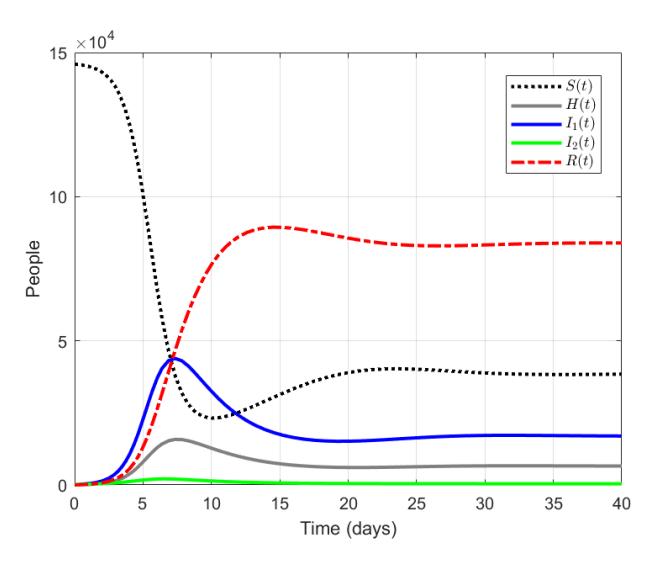
Figure 4: Simulation of rumor spread dynamics in the proposed model (1).
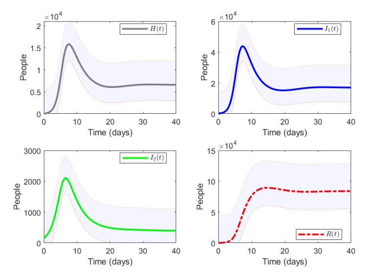
Figure 5: Simulation of subpopulations: H(t), I1(t), I2(t), and R(t) in Model (1).
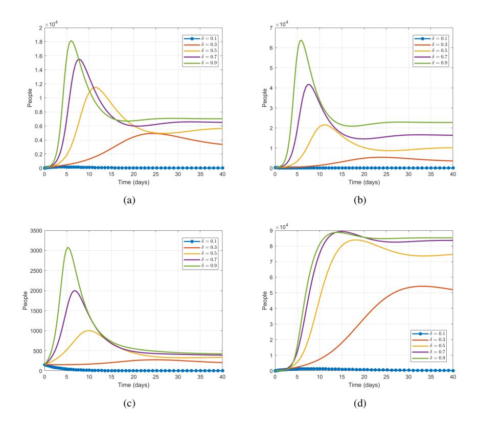
Figure 6: Sensitivity of Model (1), subpopulations: (a) H(t), (b) I1(t), (c) I2(t), and (d) R(t) with δ variations.
If we observe the rumor dynamics in more in-depth, as shown in Figure (4), the number of susceptible people who had not heard any rumors immediately decreases significantly within the first ten days. During this period, the rumors begin to spread rapidly and circulate through society, leading to an increase in the hesitated, affected, and resistant subpopulations. Since α1 > α2, the number of people affected by the rumor related to candidate 1, who also become become spreaders, is higher than those affected by the rumor related to candidate 2. Meanwhile, the number of hesitated people consistently remains between the number of people affected by rumors about candidate 1 and candidate 2. Additionally, a considerable number of people shift from being both hesitant and affected to becoming disbelievers, losing interest in spreading the rumors. This is evidenced by the increasing number of resistant people in Figure (4), which tends to be stable after twenty days.
Thirdly, we performed simulations to analyze the sensitivity of the rumor model (1) with respect to changes in the parameter δ. To conduct this simulation, we varied the δ values as follows: δ = 0.1, δ = 0.3, δ = 0.5, δ = 0.7, and δ = 0.9, then simulated the rumor dynamics of the subpopulations in Model (1), as shown in Figure (6). Based on Figure 6(a)-(d), we can observe that the number of hesitated, affected, and resistant people increases in a relatively short period as the δ value grows. However, in the hesitated and affected subpopulations as shown in Figure 6(a)-(c), the number of people immediately decreases due to shift in public attitudes, resulting in more people becoming resistant to the rumors. This can be observed from the large number of resistant people in Figure 6(d), which tend to be stable after a certain number of days. Thus, this simulation confirms the sensitivity analysis that has been conducted analytically in the previous section, an increase in δ leads to an increase in R0. Nevertheless, at lower values of δ, such as δ = 0.1, the impact on the rumor dynamics in society is tends minimal.
Finally, we aim to observe the dynamics of each subpopulation when the conditions of α1 are varied, either for α1 < α2 or α1 > α2. Therefore, we performed simulations of the rumor model (1) to analyze
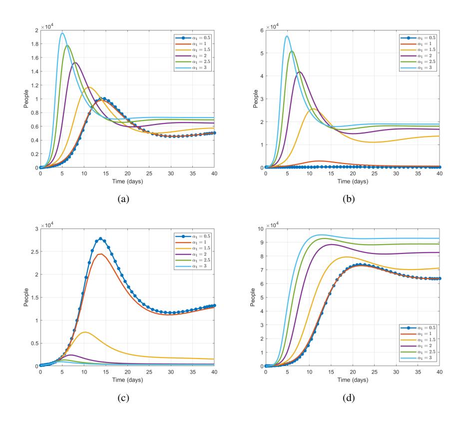
Figure 7: Sensitivity of Model (1), subpopulations: (a) H(t), (b) I1(t), (c) I2(t), and (d) R(t) with α1 variations.
its sensitivity with respect to changes in parameter α1. To conduct this simulation, we varied the α1 values as follows: α1 = 1, α1 = 1.5, α1 = 2, α1 = 2.5, and α1 = 3, then simulated the rumor dynamics of the subpopulations in Model (1), as shown in Figure (7).
Based on Figure (7), we can observe some of the rumor dynamics that occur within each subpopulation. In Figure 7(a), it can be observed that higher values of α1 result in a greater number of people becoming hesitant in a relatively short period. Figure 7(b) clearly shows that the dynamics of people affected by rumors about candidate 1 decreases as α1 decreases. Even when α1 value is significantly smaller than α2, in this case α1 = 0.5, there is no significant impact on the dynamics of I1. Conversely, lower values of α1 lead to higher dynamics of I2 within the first fifteen days, as shown in Figure 7(c). Furthermore, in subsequent time periods, the dynamics of hesitated and affected people decreases due to a change in people's attitude become resistant to rumors. Consequently, the number of resistant people increases with the higher values of α1, and tends to be stable rapidly as shown in Figure 7(d).
5. CONCLUSION
Mathematical models offer a more in-depth understanding of various aspect in life, including the social dynamics that occur within society. In this study, we formulated a mathematical model of the rumor spread dynamics in the context of an election. The model was constructed as a system of ordinary differential equations, with the human population is divided into five subpopulations as compartments. The model captures three distinct attitudes people when heard the rumors about two candidates: hesitation, being affected, and resistance, within the electoral context.
We determined R0 as the threshold for rumor spread in society. Through numerical experiments, we obtained that the rumor free equilibrium is locally asymptotically stable when R0 < 1, while the rumor existence equilibrium is locally asymptotically stable when R0 > 1. The sensitivity analysis of R0 was also conducted to identify the most influential parameter in the proposed model to R0 dynamics. This analysis revealed that an increase in the parameter δ which represent the proportion of susceptible people becoming affected, plays a crucial role in the rise of R0. Furthermore, we can conclude that the proportion of susceptible people becoming affected people followed by the higher rumor transmission rate for one candidate compared to the other, is a necessary and sufficient condition for the rumor about a candidate to continue circulating in society. This analysis can be considered as a campaign strategy in an electoral context [24].
Dynamically, the spread of rumors can be effectively captured through several numerical simulations of the proposed model. The simulations reveal that the number of hesitant people will consistently remain between the two groups of affected people or rumor spreader for two candidates. These two subpopulations increase rapidly at the beginning of the time period and after reaching a maximum will decrease immediately. This occurs because people become resistant to the rumors within a short time period and then remain stable at a certain time. Therefore, we can conclude that in the electoral context, rumors about candidates will continuously develop and circulate in society during this time period. Psychologically, this is supported by the natural tendency of people who need fact finding and social reinforcement when confronted with rumors [1], [25]. Additionally, another interesting aspects is the large number of people who become resistant or disbelieve the rumors. This can be interpreted positively as a critical and reasonable attitude from the public toward rumors about candidates [11], [38].
Variations in the model parameters also influence the dynamics of rumors. Simulations show that the hesitant, affected, and resistant subpopulation increase rapidly when the proportion of susceptible people who become affected people rises, along with an increase in the rumor transmission rate. Even a small proportion is insufficient to enable rumors to develop and circulate within society. Therefore, in the context of an electoral race, these two aspects should be considered collectively. For instance, when attempting to persuade the public during campaigns, debates, or other electoral activities, it is crucial to address both factors [10], [24].
While the dynamics of rumor spread have been explored in this study, the proposed model can be further developed for deeper insight. Future research could consider to incorporate other possible attitudes of people and media factors towards rumors. Additionally, utilizing different case studies could provide varied perspectives on the dynamics of rumor spread within society.
ACKNOWLEDGEMENT
The authors express their gratitude to the editor and reviewers for their insightful comments and suggestions. The authors also thank to Unggulan and LPDP Scholarship from the Ministry of Education and the Ministry of Finance for supporting the Master's Program at Institut Teknologi Bandung. This research was supported by a research grant from Institut Teknologi Bandung.