

1. Introduction
Tuberculosis (TB) remains one of the earliest disease to plague humanity. It has been proclaimed to be a global pandemic by the World Health Organization. This disease remains among the top killer diseases despite advances in science. TB is a respiratory disease primarily targeting the lungs and it is transmitted through the air. It is estimated that M. Tuberculosis infects about one-third of the global population, of which some may progress into active TB. A large proportion of TB patients are found in most parts of Africa and the southern parts of east Asia (see [1]). TB is transmitted majorly through close contact. The bacteria responsible for TB are mostly transmitted when an infected individual coughs or sneezes [2]. There is still a long way to go in eradicating TB due to inadequate drug intake, prolonged treatment courses, and incomplete treatment [3].
Tuberculosis remains highly prevalent in Nigeria, placing it among the countries with the greatest disease worldwide. A significant rise in TB prevalence over the years is observed from data released by the National Tuberculosis, Leprosy and Buruli Ulcer Control Programme (NTBLCP) of the Federal Ministry of Health as shown in Figure 1. However, there has been an improvement in the treatment success rate since 2016 has shown in Figure 2. A steady decline in mortality ratio from 2015 to 2021, with a 26.77% rate of mortality-to-infection has been reported. Nonetheless, under-reporting significantly undermines disease surveillance efforts and continues to drive the rising transmission risk. An undetected TB case is estimated to potentially infect around 15 people annually [4].
There are various TB models depending on the objectives of the researcher. Guo et al [5] examined the global stability in a TB model by incorporating both latent and clinical stages. The major results obtained
*Corresponding author
Received June \(4^{th}\), 2024, Revised March \(19^{th}\), 2025, Accepted for publication June \(15^{th}\), 2025. Copyright ©2025 Published by Indonesian Biomathematical Society, e-ISSN: 2549-2896, DOI:10.5614/cbms.2025.8.1.4
included TB-free and persistence equilibrium dynamics. Faniran et al [6] applied SIR mathematical dynamics to investigate tuberculosis among health workers by incorporating vaccination and respirator compliance. Sulayman et al [7] used a modified TB model to examine dynamical behaviour of the impact of hospital treatment and public health education. Simorangkir [8] considered tuberculosis dynamics consisting of observed treatments and vaccination. Wang et al. [9] considered the latent class of TB in their co-infection model of TB and HIV. Latent TB means the bacteria are dormant in the person; thus, the person is not ill and not infectious. However, there can be transition from latent TB to active TB, where the person begins to shows symptoms. A tuberculosis model with three infected classes was examined by [10]. The diseased class is split into asymptomatic, symptomatic, and drug-resistant populations.
Isolation as a control strategy for some infectious diseases was examined by (see [11], [12], [13]). Isolation is a control measure by which infectious persons are removed from the population to prevent the infection from spreading further [14].
In this research, we use an SIQR(Susceptible, Infected, Isolated, Recovered) mathematical model to investigate TB dynamics. In the model, infected individuals are categorized as either asymptomatic or symptomatic, with the possibility of moving to either class from the susceptible class. The remainder of the paper is put together as follows: The description of the model is considered in Section 2, while the formulated model is thoroughly analyzed and discussed in Section 3. Numerical simulation and the conclusion of our paper are presented in Sections 4 and 5, respectively.
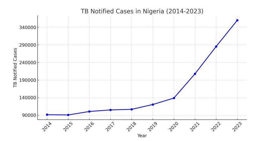
Figure 1: TB notification cases.
2. MODEL FORMULATION
Mathematical modeling is pivotal to gaining insight into disease evolution and dynamics in order to formulate effective control policies. The human population is split into five compartments in this study. The susceptible class is represented by S; the asymptomatic compartment is denoted by IA; the symptomatic class is denoted by IS; the isolated compartment is captured using Q; while recovered compartment is captured using R. The susceptible compartment experiences an increase in population through migration, and this rate is captured using Λ. The susceptible compartment is reduced via interaction with symptomatic individuals at rate β, with a fraction ρ being asymptomatic and (1 − ρ) being symptomatic. The asymptomatic individuals become symptomatic at rate α1 and get recovered at rate γ1. The symptomatic population experiences death caused by TB at rate δ1, and recovery at rate γ2, while the rest are isolated at rate α2. The isolated population also experiences death caused by TB at rate δ2 and recovery at rate γ3. Every segment of the population at
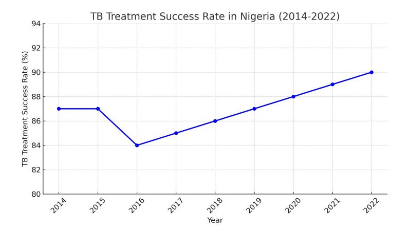
Figure 2: TB Treatment treatment success rate.
rate \(\mu\) experiences natural death. The dynamics of the model are represented below using Equations (1) - (5).
\[\frac{dS}{dt} = \Lambda - \beta S I_S - \mu S,\tag{1}\]
\[\frac{dI_A}{dt} = \rho \beta SI_S - (\alpha_1 + \gamma_1 + \mu)I_A, \tag{2}\]
\[\frac{dI_S}{dt} = (1 - \rho)\beta SI_S + \alpha_1 I_A - (\alpha_2 + \gamma_2 + \mu + \delta_1)I_S, \tag{3}\]
\[\frac{dS}{dt} = \Lambda - \beta S I_S - \mu S, \tag{1}\] \[\frac{dI_A}{dt} = \rho \beta S I_S - (\alpha_1 + \gamma_1 + \mu) I_A, \tag{2}\] \[\frac{dI_S}{dt} = (1 - \rho) \beta S I_S + \alpha_1 I_A - (\alpha_2 + \gamma_2 + \mu + \delta_1) I_S, \tag{3}\] \[\frac{dQ}{dt} = \alpha_2 I_S - (\gamma_3 + \mu + \delta_2) Q, \tag{4}\] \[\frac{dR}{dt} = \gamma_1 I_A + \gamma_2 I_S + \gamma_3 Q - \mu R, \tag{5}\]
\[\frac{dR}{dt} = \gamma_1 I_A + \gamma_2 I_S + \gamma_3 Q - \mu R,\tag{5}\] and initial conditions \(S(0) \ge 0, I_A(0) \ge 0, I_S(0) \ge 0, Q(0) \ge 0, R(0) \ge 0.\)
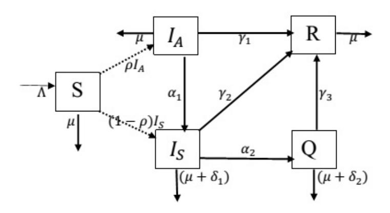
Figure 3: Diagram illustrating the model dynamics.
| Definition | Parameters | Value | Source |
|---|---|---|---|
| Recruitment rate into the susceptible class | Λ | 0.6 | Assumed |
| TB transmission rate | β | 0.12 | [15] |
| Natural death rate | \(\mu\) | 0.02041 | [ |
| Progression rate to symptomatic class | \(\alpha_1\) | 0.06 | [16] |
| Progression rate to isolated class | \(\alpha_2\) | 0.3 | Assumed |
| Recovery rate from \(I_A\) class | \(\gamma_1\) | 0.3 | Assumed |
| Recovery rate from \(I_S\) class | \(\gamma_2\) | 0.0575 | [17] |
| Recovery rate from \(Q\) class | \(\gamma_3\) | 0.1106456 | [17] |
| Rate of TB death arising from the \(I_A\) class | \(\delta_1\) | 0.01 | [17] |
| Rate of TB death arising from the \(Q\) class | \(\delta_2\) | 0.0575 | [17] |
Table 1: Model parameters and values.
3. MODEL ANALYSIS
The system is qualitatively analyzed for better understanding of the dynamical features of TB dynamics.
3.1. Positivity of solutions
Human population cannot be negative. It is therefore necessary for the positivity of the state variables to be ascertained for future time.
Theorem 3.1. (Positivity of solutions). The set of solutions of S(t), \(I_A(t)\), \(I_S(t)\), Q(t), R(t) of System (1) - (5) are positive for \(t \ge 0\) with initial conditions S(0), \(I_A(0)\), \(I_S(0)\), Q(0), R(0) being nonnegative.
Proof: From (1), we obtain
\[\frac{dS}{dt} \ge -\beta S I_S - \mu S. \tag{6}\]
Equation (6) is solved as:
\[S(t) \ge S(0)e^{-\left[\beta \int I_S(\tau)d\tau + \mu t\right]} \ge 0. \tag{7}\]
The same technique is applied to establish that \(I_A(t) \ge 0, I_S(t) \ge 0, Q(t) \ge 0\), and \(R(t) \ge 0\) for future time. Thus, positivity of the state variables is ascertained for future time.
3.2. Invariant region
The region where the solution of the model is bounded is established.
Theorem 3.2. (Invariant region). The region \(\Omega = \{S(t), I_A(t), I_S(t), Q(t), R(t) \in \mathbb{R}^5_+ : N(0) \leq N(t) \leq \frac{\Lambda}{\mu} \}\) is positive invariant for system (1) - (5) given that the initial conditions are nonnegative.
Proof: Differentiating the total human population \(N(t) = S(t) + I_A(t) + I_S(t) + Q(R) + R(t)\) gives
\[\frac{dN}{dt} = \Lambda - \mu N - \delta_1 I_S - \delta_2 Q. \tag{8}\]
Further simplification gives
\[\frac{dN}{dt} \le \Lambda - \mu N. \tag{9}\]
Solving the differential inequality (9) together with the initial condition gives
\[0 \le N(t) \le \left(N(0)e^{-\mu t} + \frac{\Lambda}{\mu}(1 - e^{-\mu t})\right). \tag{10}\]
Taking the limit as \(t \to \infty\) gives,
\[N(0) \le N(t) \le \frac{\Lambda}{\mu}.\tag{11}\]
Hence, every solution for all time t in \(\Omega\) remains in \(\Omega\). Thus, \(\Omega\) remains unchanged over time ensuring the epidemiological and mathematical feasibility of the region.
3.3. Disease-free equilibrium
Solving \(\frac{dS}{dt}=\frac{dI_A}{dt}=\frac{dI_S}{dt}=\frac{dQ}{dt}=\frac{dR}{dt}=0\) coupled with \(I_A(t)=I_S(t)=Q(R)=0\) gives TB-free equilibrium solution of the system. It is represented below as
\[\pi_0 = \left(S^0(t), I_A^0(t), I_S^0(t), Q^0(t), R^0(t)\right) = \left(\frac{\Lambda}{\mu}, 0, 0, 0, 0, 0\right). \tag{12}\]
3.4. Basic reproduction number
The basic reproduction number \((R_0)\) describes the expected value of secondary cases generated when one infectious case is introduced into a population that is entirely susceptible. The method by Van den Driessche and Watmough [18] is utilized to determine \((R_0)\). The emergence rate of new TB cases is denoted by \(\mathcal{F}\), while TB transfer rate among the compartments is represented by V.
Let \(x = (I_A, I_S, Q)^T\), we can thus write Equations (2) - (4) such that \(\dot{x} = \mathcal{F}(x) - \mathcal{V}(x)\) where
\[\mathcal{F} = \left( \begin{array}{c} \rho \beta S I_S \\ (1 - \rho) \beta S I_S \\ 0 \end{array} \right), \quad \mathcal{V} = \left( \begin{array}{c} (\alpha_1 + \alpha_1 + \mu) I_1 \\ -\alpha_1 I_A + (\alpha_2 + \gamma_2 + \mu + \delta_1) I_S \\ -\alpha_2 I_S + (\gamma_3 + \mu + \delta_2) Q \end{array} \right).\]
The Jacobian matrices of \(\mathcal{F}\) and \(\mathcal{V}\) with respect to \(I_A, I_S\) and Q respectively at \(\pi_0\) gives
\[F = \begin{pmatrix} 0 & \frac{\rho\beta\Lambda}{\mu} & 0 \\ 0 & \frac{(1-\rho)\beta\Lambda}{\mu} & 0 \\ 0 & 0 & 0 \end{pmatrix}, \quad V = \begin{pmatrix} (\alpha_1 + \gamma_1 + \mu) & 0 & 0 \\ -\alpha_1 & (\alpha_2 + \gamma_2 + \mu + \delta_1) & 0 \\ 0 & -\alpha_2 & (\gamma_3 + \delta_2 + \mu) \end{pmatrix}.\]
\(R_0\) is explicitly computed using \(\rho(FV^{-1})\), where \(\rho\) signifies the spectral radius. Hence,
\[R_0 = \frac{\beta \Lambda [\alpha_1 \rho + (1 - \rho)(\alpha_1 + \gamma_1 + \mu)]}{\mu(\alpha_1 + \gamma_1 + \mu)(\alpha_2 + \gamma_2 + \mu + \delta_1)}.\] (13)
3.5. Local stability of disease-free equilibrium
Theorem 3.3. TB-free equilibrium is locally asymptotically stable for the system (1) - (5) provided that \(R_0 < 1.\)
Proof: The stability dynamics of the system is studied by obtaining the variational matrix of the system. The variational matrix of (1) - (5) at \(\pi_0\) gives
\[J(\pi_0) = \begin{pmatrix} -\mu & 0 & -\frac{\beta\Lambda}{\mu} & 0 & 0\\ 0 & -(\alpha_1 + \gamma_1 + \mu) & \frac{\rho\beta\Lambda}{\mu} & 0 & 0\\ 0 & \alpha_1 & \frac{(1-\rho)\beta\Lambda}{\mu} - (\alpha_2 + \gamma_2\mu + \delta_1) & 0 & 0\\ 0 & 0 & \alpha_2 & -(\gamma_3 + \mu + \delta_2) & 0\\ 0 & \gamma_1 & \gamma_2 & \gamma_3 & -\mu \end{pmatrix}.\]
The following eigenvalues are obtained from \(J(\pi_0)\) easily
\[\lambda_1 = -\mu\]
\[\lambda_2 = -\mu\]
\[\lambda_2 = -\mu, \lambda_3 = -(\gamma_3 + \mu + \delta_2),\]
The reduced matrix \(J(\pi_0^*)\) below is used to obtain the remaining two eigenvalues.
\[J(\pi_0^*) = \begin{pmatrix} -(\alpha_1 + \gamma_1 + \mu) & \frac{\rho\beta\Lambda}{\mu} \\ \alpha_1 & \frac{(1-\rho)\beta\Lambda}{\mu} - (\alpha_2 + \gamma_2\mu + \delta_1) \end{pmatrix}.\]
The characteristic equation yields negative eigenvalues if \(J(\pi_0^*)\) has a negative trace and a positive determinant. Det\((J(\pi_0^*))=(\alpha_1 + \gamma_1 + \mu)(\alpha_2 + \gamma_2 \mu + \delta_1)(1 - R_0)\), which is positive if \(R_0 < 1\).
Thus, the TB-free equilibrium remains locally asymptotically stable provided that \(R_0 < 1\) is satisfied.
3.6. Existence of endemic equilibrium
TB endemic equilibrium is a positive fixed point solution where there is persistence of TB within the system.
Theorem 3.4. An endemic equilibrium exists in the population provided that \(R_0 > 1\).
Proof: The notation \(E^* = (S^*, I_A^*, I_S^*, Q^*, R^*)\) is used to denote the system's endemic equilibrium. The persistence equilibrium of (1) - (5) is given by
\[S^* = \frac{\Lambda}{\mu R_0},\tag{14}\]
\[I_S^* = \frac{\mu(R_0 - 1)}{\beta},\] (15)
\[I_A^* = \frac{\rho \Lambda(R_0 - 1)}{R_0(\alpha_1 + \gamma_1 + \mu)},\] (16)
\[Q^* = \frac{\alpha_2 \mu (R_0 - 1)}{\beta (\gamma_3 + \mu + \delta_2)}, \tag{17}\]
\[R^* = \left(\frac{\gamma_1 \rho \Lambda}{\mu R_0(\alpha_1 + \gamma_1 + \mu)} + \frac{\gamma_3}{\beta} + \frac{\gamma_3 \alpha_2}{\beta(\gamma_3 + \mu + \delta_2)}\right) (R_0 - 1). \tag{18}\]
3.7. Global stability
The global asymptotic stability property of \(\pi_0\) for the TB model is explored.
Theorem 3.5. The disease-free equilibrium of system (1) - (5) is globally asymptotically stable if \(R_0 \le 1\).
Proof: The global stability is demonstrated using the Lyapunov function presented below.
\[V = \alpha_1 I_A + (\alpha_1 + \gamma_1 + \mu) I_S, \tag{19}\]
Differentiating and substituting \(\dot{I}_A\) and \(\dot{I}_S\) gives
\[\dot{V} = \alpha_1 [\rho \beta S I_S - (\alpha_1 + \gamma_1 + \mu) I_A] + (\alpha_1 + \gamma_1 + \mu) [(1 - \rho) \beta S I_S + \alpha_1 I_A - (\alpha_2 + \gamma_2 + \mu + \delta_1) I_A].\] (20) Simplifying gives
\[\dot{V} = \alpha_1 \rho \beta S I_S + (1 - \rho)(\alpha_1 + \gamma_1 + \mu)\beta S I_S - (\alpha_1 + \gamma_1 + \mu)(\alpha_2 + \gamma_2 + \mu + \delta_1)I_A. \tag{21}\]
We thus obtain
\[\dot{V} \le (\alpha_1 + \gamma_1 + \mu)(\alpha_2 + \gamma_2 + \mu + \delta_1)[R_0 - 1]I_A.\]
We conclude that \(\dot{V} \leq 0\) provided that \(R_0 < 1\) with equality if \(R_0 = 1\) or \(I_A = 0\). Hence, the singleton \(\pi_0\) is the largest invariant set in \(\{S(t), I_A(t), I_S(t), Q(t), R(t) \in \mathbb{R}^5_+\}\). Thus, as \(t \to \infty\), every solution with initial conditions in \(\mathbb{R}^5_+\) of (1) - (5) converges to \(\pi_0\) by the LaSalle invariance principle [19].
3.8. Sensitivity analysis
Sensitivity analysis measures the responsiveness of the system structure to fluctuations in the parameter values of the system. Given a variable q relative to \(R_0\), the normalized forward sensitivity index is given as:
\[\Upsilon_q^{R_0} = \frac{\partial R_0}{\partial q} \times \frac{q}{R_0}.\] (22)
A direct variation between the parameter and \(R_0\) gives a positive sensitivity index, while an indirect relationship gives a negative index. The computation of the sensitivity index is obtained using (22), and the result is presented in Table 2. It is evident from Table 2 that \(R_0\) of the parameters \((\beta, \Lambda, \alpha_1)\) will increase as the value of the parameters rise since they have positive indices. Parameters with negative indices \((\gamma_1, \gamma_2, \alpha_2, \delta_1)\), will reduce the basic reproduction number as their value increases. From Table 2, \(\Upsilon_{\Lambda}^{R_0} = 1\) implies that an increase in \(\Lambda\) by 5% will produce an increase of 5% in \(R_0\). Similarly, a decrease in \(\Lambda\) by 5% will produce a decrease of 5% in \(R_0\).
Parameter β Λ \(\alpha_1\)\(\gamma_1\)\(\alpha_2\)\(\gamma_2\)\(\delta_1\)\((\alpha_2+\gamma_2+\mu+\delta_1)\)
Table 2: Sensitivity index.
3.9. Optimal control application
In this section, isolation is incorporated as a control function into model (1) - (5) to determine its effectiveness in reducing the impact of TB in the system. Our strategy focuses on the control of TB by introducing an isolation control function u(t) into the system (1) - (5). The percentage of the symptomatic population being isolated within a given time frame is denoted using u(t). The extended model with control thus becomes:
\[\frac{dS}{dt} = \Lambda - \beta S I_S - \mu S,\tag{23}\]
\[\frac{dI_A}{dt} = \rho \beta S I_S - (\alpha_1 + \gamma_1 + \mu) I_A, \tag{24}\]
\[\frac{dS}{dt} = \Lambda - \beta S I_S - \mu S, \tag{23}\] \[\frac{dI_A}{dt} = \rho \beta S I_S - (\alpha_1 + \gamma_1 + \mu) I_A, \tag{24}\] \[\frac{dI_S}{dt} = (1 - \rho) \beta S I_S + \alpha_1 I_A - (\alpha_2 + u + \gamma_2 + \mu + \delta_1) I_S, \tag{25}\] \[\frac{dQ}{dt} = (\alpha_2 + u) I_S - (\gamma_3 + \mu + \delta_2) Q, \tag{26}\] \[\frac{dR}{dt} = \gamma_1 I_A + \gamma_2 I_S + \gamma_3 Q - \mu R. \tag{27}\]
\[\frac{dQ}{dt} = (\alpha_2 + u)I_S - (\gamma_3 + \mu + \delta_2)Q, \tag{26}\]
\[\frac{dR}{dt} = \gamma_1 I_A + \gamma_2 I_S + \gamma_3 Q - \mu R. \tag{27}\]
This strategy has the goal of reducing the symptomatic population and isolated population at minimum possible cost. The execution within the time horizon [0,T] of control u(t) solves this minimization problem. The objective functional denoted by J(u) is represented as
\[\int_0^T (pI_S + qQ + nu^2) \, dt. \tag{28}\]
The final time is represented by T and positive weights parameters p, q, n are to balance the factors. The state system is considered within admissible set of control functions
\[\mathcal{U} = \left\{ u \in L^{1}(0, T) \mid 0 \le u \le 1 \forall t \in [0, T] \right\}. \tag{29}\]
Hence, \(u^*\) is obtained as an optimal control satisfying
\[J(u^*) = \min\{J(u) : u \in \mathcal{U}\}. \tag{30}\]
The existence of (30) is obtained by applying the findings by Fleming and Rishel [20]. The procedure is exemplified in [21], [22], and [23].
Pontryagin's Maximum Principle [24] is applied to reformulates equations (23) - (30) into a minimization problem involving a Hamiltonian function \(\mathcal{H}\) in order to determine the necessary conditions of the optimal control problem. The Hamiltonian function \(\mathcal{H}\) given as:
\[\mathcal{H}=pI_S+qQ+nu^2+\lambda_1\left[\Lambda-\beta SI_S-\mu S\right]+\lambda_2\left[\rho\beta SI_S-(\alpha_1+\gamma_1+\mu)I_A\right]\\ +\lambda_3\left[(1-\rho)\beta SI_S+\alpha_1I_A-(u+\gamma_2+\mu+\delta_1)I_S\right]+\lambda_4\left[uI_S-(\gamma_3+\mu+\delta_2)Q\right]+\lambda_5\left[\gamma_1I_A+\gamma_2I_S+\gamma_3Q-\mu R\right].\] where the adjoint variables attached to the corresponding states are \(\lambda_1,\lambda_2,\lambda_3,\lambda_4,\lambda_5\).
Theorem 3.6. (Characterization of Optimal control). There exists adjoint variables \(\lambda_1, \lambda_2, \dots, \lambda_5\) such that solutions \(S^*(t), I_A^*(t), I_S^*(t), Q^*(t)\), and \(R^*(t)\) of corresponding state system (1) - (5), and optimal control \(u^* \in \mathcal{U}\) satisfy
\[\begin{split} \frac{d\lambda_1}{dt} &= \beta I_S(\lambda_1 - \rho \lambda_2 - (1 - \rho)\lambda_3) + \lambda_1 \mu. \\ \frac{d\lambda_2}{dt} &= (\alpha_1 + \gamma_1 + \mu)\lambda_2 - \alpha_1 \lambda_3. \\ \frac{d\lambda_3}{dt} &= -p + \beta S(\lambda_1 - \rho \lambda_2 - (1 - \rho)\lambda_3) + (u + \gamma_2 + \mu + \delta_1)\lambda_3 - u\lambda_4 - \gamma_2 \lambda_5. \\ \frac{d\lambda_4}{dt} &= -q + (\gamma_3 + \mu + \delta_2)\lambda_4 - \gamma_3 \lambda_5. \\ \frac{d\lambda_5}{dt} &= \mu \lambda_5. \end{split}\] with the terminal conditions
\[\lambda_1(T) = 0, \lambda_2(T) = 0, \lambda_3(T) = 0, \lambda_4(T) = 0, \lambda_5(T) = 0.\] (31)
Furthermore, the optimal control \(u^*\) gives
\[u^* = min\left(u_{max}, max\left(0, \frac{(\lambda_3 - \lambda_4)I_S}{2n}\right)\right).\]
Proof: The adjoint equation is obtained using Pontryagin's Maximum Principle such that \(\frac{\partial \lambda_i}{\partial t} = -\frac{\partial \mathcal{H}}{\partial j}\) where, \(i = 1, 2, \dots, 5\) and \(j = S, I_A, I_S, Q, R\). Solving the optimality condition \(\frac{\partial \mathcal{H}}{\partial u} = 0\) and applying the bounds in \(\mathcal{U}\) gives the optimal control characterization.
4. NUMERICAL SIMULATION
Table 1 provides the parameter values used to carry out numerical simulation of the optimal control, with initial values \(S(0)=1000, I_A(0)=100, I_S(0)=70, I_3(0)=10\), and R(0)=0. Isolation is used as a control to optimize the objective function and the obtained results are shown in Figures 4 - 6. The numerical simulation demonstrates that implementing isolation as a control measure leads to a noticeable decline in the peak of the infected symptomatic class. In contrast to the scenario without control, where infections reach a higher peak, isolation significantly curtails disease spread by minimizing interactions between infected and susceptible individuals. This effect is clearly depicted in Figure 4.
Moreover, as isolation is enforced, the population of isolated class rises accordingly. This expected trend, illustrated in Figure 5, underscores the role of isolation in limiting disease transmission. By reducing direct exposure, isolation serves as an effective intervention in managing the spread of infection. Additionally, the impact of isolation extends to recovery outcomes. The results indicate an improvement in the recovered class when compared to the uncontrolled scenario as shown in Figure 6. Since isolation lowers the infection burden, more individuals receive timely medical attention, increasing recovery rates. This highlights the broader benefits of isolation, not only in reducing infection levels but also in enhancing overall disease control efforts. This is key to improving treatment success rate.
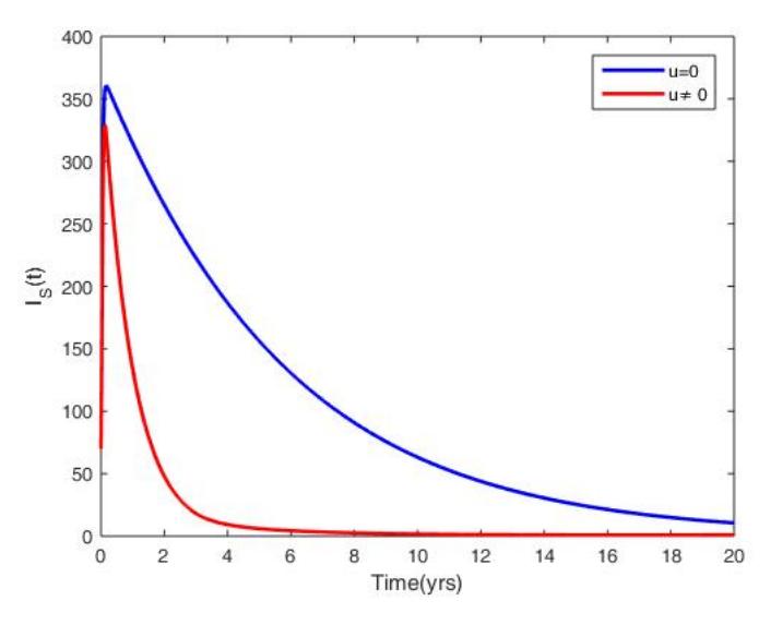
Figure 4: Simulation dynamics displaying the impact of the control on Infected Symptomatic compartment.
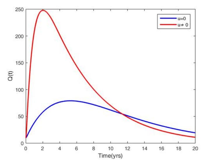
Figure 5: Simulation dynamics displaying the impact of the control on Isolated compartment.
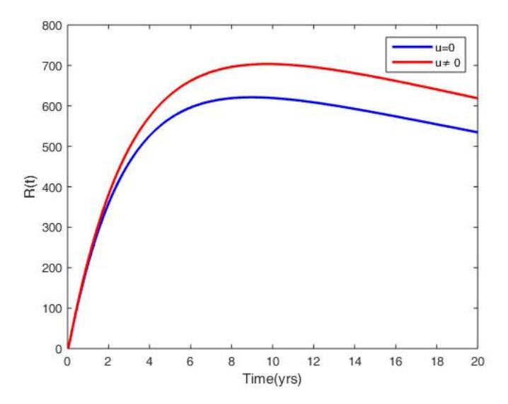
Figure 6: Simulation dynamics displaying the impact of the control on Recovered compartment.
5. CONCLUSION
The mathematical model of TB dynamics is carried out in this paper using the SIQR mathematical model by incorporating both symptomatic and asymptomatic infected individuals. The model was rigorously examined to ascertain its well-posedness through positivity and invariant region analysis, ensuring that the solution of the model remain epidemiological meaningful over time. A key component of our analysis was obtaining the basic reproduction number which serves as a threshold parameter measuring TB persistence or eradication. The disease-free equilibrium was obtained, and its stability conditions were derived, showing that TB can be eliminated when R0 < 1. Conversely, endemic equilibrium exists for R0 > 1 signifying the persistence of infection within the population. The sensitivity analysis provided insight regarding the influence of key epidemiological parameters on TB transmission dynamics. This analysis highlighted that parameters associated with asymptomatic carriers play a substantial role in sustaining TB infections, reinforcing the need for targeted interventions.
A pivotal aspect of this research was the incorporation of optimal control theory, where isolation was examined as the sole control measure. The optimization framework was structured to minimize both the number of symptomatic and isolated population. Numerical simulations demonstrated that strategic and timely implementation of isolation significantly reduces disease prevalence, particularly when effectively applied to symptomatic individuals. These findings underscore the profound impact of strict isolation measures in breaking transmission chains and increasing recovery rates.
ACKNOWLEDGEMENT
The authors appreciate the reviewers' efforts in enhancing the paper.