

1. INTRODUCTION
Besides water and air, food is one of the most essential requirements for sustaining life. Since ancient times, humans have always prioritized obtaining food, whether through traditional home-cooked meals or modern fast food outlets. Fast food consumption can become addictive, similar to smoking, drinking, or substance abuse. Today, fast food addiction has become a widespread social phenomenon, affecting societies in both developed and developing nation. Fast food appeals to people of all ages, cultural backgrounds, and socioeconomic levels. However, it is particularly popular among young people and teenagers.
The change in the lives of individuals today, which I research, is characterized by speed of life and work, as well as the transformation of the roles, of men and women in their daily lives and women working daily and spending long hours outside the home, and delayed sleep schedules among parents and subtle media campaigns The distance between the workplace and the accommodation for workers, students, and pupils has led individuals to rely on fast food for their daily lunch. All of these factors led to the increase in eating out at restaurants, especially those that provide fast food, which became a major reason why children and families without considering the negative effects of frequent fast food consumption. A 2016 WHO report indicates that more than 650 million adults aged 18 and over were classified as obese. Among adults, obesity rates were 11% for men and 15% for women. The global obesity rate nearly tripled from 1975 to 2016 [24]. By 2016, overweight and obesity impacted around 41 million children under five years of age. This issue, once more common in rich countries, is increasingly affecting developing countries, particularly in urban areas. In Africa, overweight rates among children under five have experienced a notable surge, nearly 50% since 2000, and nearly half of obese children under 5 reside in Asia. Furthermore, as of 2016, more than 340 million adolescents between the ages of 5 and 19 fell into the overweight category. Overweight and obesity now lead to more deaths worldwide than underweight does, with global figures showing more obese individuals than underweight ones, except in certain regions of sub-Saharan Africa and Asia.
During 2015-2016, 39.8% adults in the U.S. were obese, affecting about 93.3 million people. Obesity was most common in adults aged 40-59 42.8% over 41.0% among those aged 60, and 35.7% among those aged
*Corresponding author
Received June 6th, 2024, Revised November 12th, 2024, Accepted for publication May 31st, 2025. Copyright ©2025 Published by Indonesian Biomathematical Society, e-ISSN: 2549-2896, DOI:10.5614/cbms.2025.8.1.5 20-39. From 1999-2000 to 2015-2016, obesity rates significantly increased among both U.S. adults and youth, though the change between 2013-2014 and 2015-2016 was not significant. In Morocco, the total number of obese adults over 18 increased from 5.3 million in 2004 to 7 million in 2014, mirroring a global trend of rising adult obesity (see [14]).
According to a Food and Agriculture Organization (FAO) report, published in September 2018, fast food is widespread in Pacific small island developing countries, where most of their food must be imported. The obesity rate among women in Fiji is over 30%, and in American Samoa it is as high as 80%. In at least 10 pacific countries, more than half of the population (some even reaching 90%) is overweight, primarily due to the overconsumption of imported processed foods rich in sugar, salt, and trans fats. Currently, an estimated 2.6 billion individuals are overweight, and global obesity prevalence has risen from 11.7% in 2012 to 13.2% in 2016. Health authorities should encourage a healthy and diversified diet and support the integration of local products into the market. Initiatives like school feeding programs that connect local production with school meals can both strengthen the local economy and promote healthier diets for children, see [5].
Addiction to fast food can lead to partly due to its negative impact on cholesterol levels—specifically, raising LDL (bad cholesterol) and lowering HDL (good cholesterol). Additionally, excessive intake of fast food can contribute to obesity, which further elevates the risk of heart disease. The impact on the liver is another concern, as fat from fast food can accumulate there, potentially causing damage, infections, and even scarring. Obesity also raises the risk of diabetes, a condition where the pancreas struggles to produce sufficient insulin to convert sugars into energy, leading to increased glucose in the blood and a greater risk of type 2 diabetes. Stroke, hyperlipidemia, hypertension due to white bread and pastries, degenerative inflammation of the knees and constipation of the lungs, family damages, and overweight and obesity rates have increased significantly in recent decades, representing a health pandemic in the US and in other countries [24], [18], [14]. There are also family damages, including the dismantling of family burdens and extra family budgets. Fast food has several effects on the individual, including a shift in their relationship with his family members, a lack of interest in young people to sit with family members around one table, the spread of diseases, especially food poisoning, the lack of interest of young people in traditional dishes, increasing women's dependence on fast food for food, a change in family income, and youth spending heavily on fast food.
Numerous studies in the field psychology and social sciences have investigated these topics; see, for example, [2], [19], [23], [16] and references therein. [21] stated that the overweight/obesity prevalence rates have surged significantly in recent decades, becoming a health crisis in US. Unhealthy eating habits are one of the determinants that negatively affect weight in early adulthood. The aim of this exploratory study was to identify the factors (barriers and facilitators) that American college students believe influence healthy eating habits using a qualitative research design. Parents eating behaviors and social pressure from friends are believed to have both negative and positive effects on people's eating behaviors. The study emphasized the significance of involving college students in establishing nutritious eating patterns on campus, such as adopting healthy food options and conducting awareness campaigns. It also underscored the need to consider both individual variables and socio-ecological contexts in the evaluation [21]. Therefore, some mathematicians strive to understand and explore the obesity dynamics, reduce the harm to individuals and society, and minimize the number of obese and non-obese excessive fast food consumers. For example, Chunyoung Oh [3] studied the dynamics of an obesity model. The model shows a ahead bifurcation at the threshold value R0 = 1. If R0 < 1, obesity does not persist, wile if R0 > 1, the model has locally asymptotically stable (LAS) endemic equilibria. To control the epidemic and decrease obesity at this equilibrium, strategies were boarded, utilizing the Pontryagin maximum principle to prevent the overweight and obesity spread. Using numerical techniques, the study reveals effective control strategies, such as reducing social interaction with obese individuals or promoting exercises. In communities facing a significant obesity challenge, educational efforts and awareness campaigns emerged as particularly effective. However, lowering the social contact rate may lead to unintended consequences, like as depression and the infringement of individual rights.
Shah, N.H. et al. provide an abstract model addressing the causes of infertility linked to obesity [22]. Furthermore, by meeting all the conditions, the system demonstrated both local and global stability at the equilibrium points. The reproduction number was calculated to be 0.1752, which indicates that 17% of women are affected by infertility due to high-calorie foods. In fact, infertility tends to increase in proportion to obesity. It is impossible to avoid this risk without losing weight, making it very important to maintain health through regular physical activities or other means. Everyone should pay attention to their health to avoid future risks. This model will help educate the society to improve health awareness. D. Aldila [1] used the nonlinear mathematical XY Z model to study the connection among wholesome, overweight, and obese individuals within a random heterogeneous population. They divided the population into three categories: healthy individuals (X), overweight individuals (Y ), and obese individuals (Z). The model implemented two intervention program scenarios: healthy lifestyle exercise and nutrition program for overweight individuals and a treatment program for obese individuals. They discussed the presence and stability of both endemic and disease-free equilibria. The analysis identified a free disease equilibria, endemic equilibria, and a basic reproduction rate R0 as indicators of the epidemic R0 < 1. It was determined that the disease-free equilibria point exhibits local asymptotic stability if and only if R0 < 1. They concluded that improving the proportion of diet and treatment programs would significantly reduce R0. Since the control rate is continuous over time, the control method is employed here to determine the most effective method for increasing the overweight and obese individuals [6], [9], [10], [17]. Numerous other models have been extensively utilized to investigate this phenomenon; see, for instance, [11], [15], [13].
In this study, we use discrete-time models since statistical data is gathered at specific time intervals (days, weeks, months, and years), and the vaccination/treatment of some individuals is also administered at discrete intervals. Therefore, using discrete-time modeling is more accurate and convenient than using continuoustime modeling to describe phenomena and using discrete models to overcome some mathematical difficulties, such as the solution regularities. Therefore, difference equations (DEs) seem to be more adequate to describe epidemic models. In addition, the numerical solution of our difference system adopts discretization, which leads us to directly apply DEs. The numerical study of discrete models is relatively simple, so even nonmathematicians can easily implement it. We will also study the fast food consumption dynamics using the mathematical model PLSCQ, which categorizes fast food consumers into the following six distinct compartments: Potential consumers of fast food (P), Moderate consumers of fast food (L), Excessive consumers of fast food (S), Obese patients (C) and individuals who stop fast food consumption (Q).
Throughout this paper, we aim to identify the best approaches to reduce the number of excessive fast food consumers and obese patients, while optimizing the rate at which people quit fast food consumption. The paper attempts to showcase the underlying causes of these phenomena and identify the best prevention and treatment approaches. To this end, we employ optimal control techniques involving three interventions: 1) includes awareness campaigns targeting fast food consumers, 2) includes dietary program for excessive individuals consumers of fast food with a healthy life campaign, 3) includes the treatment for obese patients. (C).
The paper's contents are as follows: we present in Section 2, we present our discrete PLSCQ model that gouvernes the interaction among fast food consumer classes. In Sections 3-4, we address the control approach for the considered model, discussing the existence of optimal control and characterizing it using the discrete-time Pontryagin maximum principle, while Section 5 is devoted to numerical simulations.
2. MODEL SETTING AND ITS FORMULATION
We present here a discrete model PLSCQ, designed to describe the fast food consumption behaviour within a given population. The total population Nℓ := Pℓ + Lℓ + Sℓ + Cℓ + Qℓ at time ℓ is supposed to be constant. This population is assumed to be divided into five compartments, P, L, S, C, and Q, as illustrated by the diagram in Figure 1.
Let us consider the system below of the classical PLSCQ model of differential equations:
\[\begin{cases} P_{\ell+1} = b - \beta_1 \frac{P_{\ell} L_{\ell}}{N_{\ell}} + (1 - \mu) P_{\ell}, \\ L_{\ell+1} = \beta_1 \frac{P_{\ell} L_{\ell}}{N_{\ell}} + \vartheta Q_{\ell} + (1 - \mu - \beta_2) L_{\ell}, \\ S_{\ell+1} = \beta_2 L_{\ell} + (1 - \mu - \delta_1 - \alpha_1 - \alpha_2) S_{\ell}, \\ C_{\ell+1} = \alpha_1 S_{\ell} + (1 - \mu - \gamma - \delta_2) C_{\ell}, \\ Q_{\ell+1} = \alpha_2 S_{\ell} + \gamma C_{\ell} + (1 - \mu - \vartheta) Q_{\ell}, \end{cases}\] \[(1)\]
where P0 ≥ 0, L0 ≥ 0, S0 ≥ 0, C0 ≥ 0, and Q0 ≥ 0 are the initial data. Here is a description and explanation of the compartments from the previous problem:
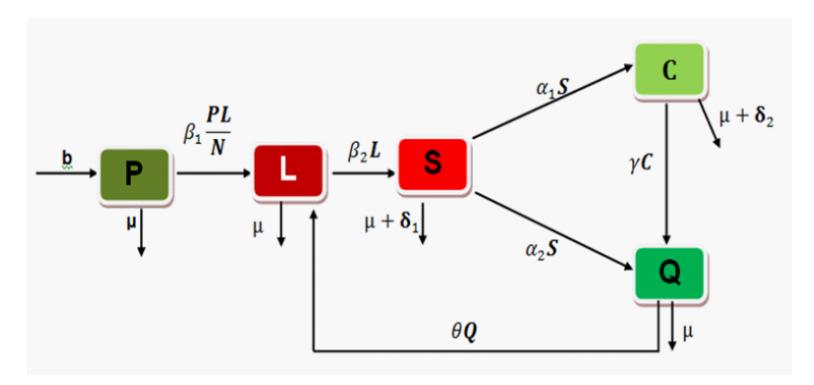
Figure 1: The PLSCQ model.
Compartment P: includes individuals who may potentially start consuming fast food. This compartment increases at the recruitment rate b and decreases due to effective interactions with moderate consumers at a rate of β1 (β1 represents the rate of transmission due to social influences on fast food consumption, including family, friends, marketing, and TV) and death rate µ. It is believed that individuals may acquire fast food consumption habits and become moderate consumers through interactions with others moderate consumers during social events such as ceremonies, weekend parties, and year-end celebrations... . In other words, it is supposed that the spread of fast-food eating habits is likened to the transmission of an infectious disease.
Compartment L: includes moderate fast food consumers who partake in fast food occasionally or in a manner not obvious to their social circles. It grows as potential individuals transition to moderate consumption with a rate parameter β1. This class diminishes when moderate-level consumers shift to excessive consumers at a rate β2 (the rate at which a moderate consumer shifts to excessive consumption) and due to natural death with rate µ.
Compartment S: includes the excessive fast food consumers. It becomes larger as the excessive fast food consumers grow with rate β2 and declines as a portion stop consuming at a rate α2 (α2 rate at which an excessive consumer of fast food individual becomes a quit from consumption of fast food) and outer becomes obesity patients (C) at rate α1(α1 rate at which a frequent fast food consumer becomes due to continuous fast food consumption). Additionally, this compartment diminishes because of death rate µ and from diseases caused by excessive fast food consumption at a rate of δ1.
Compartment C: describes the population of obese patients; this compartment increases at a rate of α1 and decreases due to γ and (µ + δ2), where γ represents the rate at which an obese individual ceases fast food consumption, and δ2 is the rate of death from obesity-related diseases caused by excessive fast food consumption.
Compartment Q: contains individuals who stop fast food consumption. This class gains individuals at a rate γ and loses them at rate ϑ (ϑ rate at which an quit and recovered individual from consumption of fast food individual becomes a moderate consumer of fast food) and µ.
3. OPTIMAL CONTROL APPROACH
This control aims to reduce the population of excessive fast food consumers and obese individuals while increasing the number of people who quit fast food and recover from obesity within the time period from ℓ = 0 to ℓ = T. Additionally, we aim to minimize the costs associated with awareness programs and treatments. To do that, we define control variables: u1 representing the efforts of awareness programs to prevent potential fast food consumers from becoming high-risk, u2 measuring the efforts of dietary programs aimed at excessive fast food consumers, promoting a healthy lifestyle, and the third control u3 measures the treatment efforts for individuals who are already obese. Furthermore, the control function ε u2 stands for
Table 1: Meaning of Parameters.
| Parameter | Meaning |
|---|---|
| b | Rate of individuals who may potentially start consuming fast food, |
| \(\beta_1\) | Rate of transmission due to social influences that leads to fast food consumption, |
| \(\mu\) | Natural death rate, |
| \(\beta_2\) | Rate of moderate consumers shift to excessive fast food consumption, |
| \(\alpha_2\) | Rate of excessive consumers of fast food quit consumption, |
| \(\alpha_1\) | Rate of frequent fast food consumer becomes obese, |
| \(\delta_1\) | Death rate from diseases caused by excessive fast food consumption, |
| \(\gamma\) | Rate of obese individual ceases fast food consumption, |
| \(\delta_2\) | Death rate from obesity-related diseases caused by excessive fast food consumption, |
| ϑ | Rate of individuals transitioning from quitting fast food to moderate consumption. |
the fraction of excessive fast food consumers who will be treated and become moderate consumers, while \((1-\varepsilon)u_2\) represents those who will receive treatment and recover from obesity. Thus, the control system is characterized by the difference equations:
\[\begin{cases} P_{\ell+1} = b - \beta_1 \frac{P_{\ell} L_{\ell}}{N_{\ell}} + (1 - \mu) P_{\ell} - u_{1,\ell} P_{\ell}, \\ L_{\ell+1} = \beta_1 \frac{P_{\ell} L_{\ell}}{N_{\ell}} + \vartheta Q_{\ell} + (1 - \mu - \beta_2) L_{\ell} + (1 - \epsilon) u_{2,\ell} S_{\ell}, \\ S_{\ell+1} = \beta_2 L_{\ell} + (1 - \mu - \delta_1 - \alpha_1 - \alpha_2) S_{\ell} - u_{2,\ell} S_{\ell}, \\ C_{\ell+1} = \alpha_1 S_{\ell} + (1 - \mu - \gamma - \delta_2) C_{\ell} - u_{3,\ell} C_{\ell}, \\ Q_{\ell+1} = \alpha_2 S_{\ell} + \gamma C_{\ell} + (1 - \mu - \vartheta) Q_{\ell} + u_{1,\ell} P_{\ell} + \epsilon u_{2,\ell} S_{\ell} + u_{3,\ell} C_{\ell}, \end{cases}\] \[(2)\]
where \(P_0\), \(L_0\), \(S_0\), \(C_0\), and \(Q_0\) were defined before. The optimal control problem associated with our model consists of minimizing the following objective function:
\[J(u_1, u_2, u_3) = S_T + C_T - Q_T + \sum_{\ell=0}^{T-1} \left[ S_\ell + C_\ell - Q_\ell + \frac{A_{1,\ell}}{2} u_{1,\ell}^2 + \frac{A_{2,\ell}}{2} u_{2,\ell}^2 + \frac{A_{3,\ell}}{2} u_{3,\ell}^2 \right], \quad (3)\]
where \(A_{1,\ell}\), \(A_{2,\ell}\), and \(A_{3,\ell}\) are non-negative parameters chosen to reflect the relative significance of the costs associated, respectively, with awareness programs, dietary programs, and treatments. The aim here is to get a control \((u_1^{op}, u_2^{op}, u_3^{op})\) verifying
\[J(u_1^{op}, u_2^{op}, u_3^{op}) = \min_{(\tilde{v}_1, \tilde{v}_2, \tilde{v}_3) \in U_{ad}} J(\tilde{v}_1, \tilde{v}_2, \tilde{v}_3), \tag{4}\] where, the subset of admissible controls \(U_{ad}\) is given by
\[U_{ad} = \{(u_1, u_2, u_3) : 0 \le u_{j\ell_{\min}} \le u_{j\ell} \le u_{j\ell_{\max}} \le 1, \ j = 1, 2, 3, \ \ell = 0, 1, \dots, T - 1\}.\] (5)
The theorem below provides criteria for the existence of an optimal control for Problems 2 and 3.
Theorem 3.1. There exists an optimal control \((u_1^{op}, u_2^{op}, u_3^{op})\) verifying
\[J(u_1^{op}, u_2^{op}, u_3^{op}) = \min_{(\tilde{v}_1, \tilde{v}_2, \tilde{v}_3) \in U_{ad}} J(\tilde{v}_1, \tilde{v}_2, \tilde{v}_3),\] (6)
under System 2 and its initial conditions.
Proof: Given the boundedness of the state coefficients, and the finiteness of the time steps, we have
\[P = (P_0, P_1, P_2, \dots, P_T), L = (L_0, L_1, L_2, \dots, L_T), S = (S_0, S_1, S_2, \dots, S_T)\]\[C = (C_0, C_1, C_2, \dots, C_T), Q = (Q_0, Q_1, Q_2, \dots, Q_T),\] are uniformly bounded for all \((u_1, u_2, u_3)\) in \(U_{ad}\). Therefore, J is a bounded functional over \(U_{ad}\), and thus
\[\inf_{(u_1, u_2, u_3) \in U_{ad}} J(u_1, u_2, u_3) < +\infty.\]
Then, there exists a sequence \((u_1^j, u_2^j, u_3^j) \in U_{ad}\) such that
\[\lim_{j \to +\infty} (u_1^j, u_2^j, u_3^j) = \inf_{(u_1, u_2, u_3) \in U_{ad}} J(u_1, u_2, u_3).\]
Consider their corresponding sequences of states \(P^j, L^j, S^j, C^j\) and \(Q^j\). Given a finitely number of bounded sequences, there exist \((u_1^{op}, u_2^{op}, u_3^{op}) \in U_{ad}\) and \(P^{op}, L^{op}, S^{op}, C^{op}, Q^{op} \in \mathbb{R}^{T+1}\) such that
\[\lim_{j \to \infty} (u_1^j, u_2^j, u_3^j) = (u_1^{op}, u_2^{op}, u_3^{op}) \,, \ \lim_{j \to \infty} P^j = P^{op},\]
\[\lim_{j \to \infty} L^{j} = L^{op} , \lim_{j \to \infty} S^{j} = S^{op} , \lim_{j \to \infty} C^{j} = C^{op} , \lim_{j \to \infty} Q^{j} = Q^{op}.\]
We recall that \((u_1^{op}, u_2^{op}, u_3^{op})\) is an optimal control with the associated states \(P^{op}\), \(L^{op}\), \(S^{op}\), \(C^{op}\) and \(Q^{op}\). Ultimately, because of the finite-dimensional nature of System 2 and the cost function J, we can derive
\[J(u_1^{op}, u_2^{op}, u_3^{op}) = \inf_{(\tilde{v}_1, \tilde{v}_2, \tilde{v}_3) \in U_{ad}} J(\tilde{v}_1, \tilde{v}_2, \tilde{v}_3).\]
4. CONTROL APPROACH AND ITS CHARACTERIZATION
We utilize the discrete form of the Pontryagin maximum principle, as described in [4], [7], [8], [20], [12] and [25]. The core concept involves introducing the adjoint functions, which connect the system of DEs to the cost function, forming the Hamiltonian functional. This principle remodels the problem of determining the optimal control into optimizing the Hamiltonian at each point while adhering to the state difference system and initial conditions.
We now write the Hamiltonian functional H, defined at time step \(\ell\), as below:
\[H_{\ell} = S_{\ell} + C_{\ell} - Q_{\ell} + \frac{A_{1,\ell}u_{1,\ell}^2}{2} + \frac{A_{2,\ell}u_{2,\ell}^2}{2} + \frac{A_{3,\ell}u_{3,\ell}^2}{2} + \sum_{i=1}^{5} \lambda_{i,\ell+1} f_{i;\ell+1},\tag{7}\] where \(f_{i;\ell+1}\) is the right-hand side of System 2 of the \(i^{th}\) state variable at time-step \(\ell+1\).
Theorem 4.1. Given a control \((u_1^{op}, u_2^{op}, u_3^{op}) \in U_{ad}\) and solutions \(P_\ell^{op}\), \(L_\ell^{op}\), \(S_\ell^{op}\), \(C_\ell^{op}\) and \(Q_\ell^{op}\) for System 2, then there are adjoint functions \(\lambda_1\), \(\lambda_2\), \(\lambda_3\), \(\lambda_4\), and \(\lambda_5\) fulfilling the conditions below
\[\lambda_{1,\ell} = \partial H_{\ell} / \partial P_{\ell} = (\lambda_{2,\ell+1} - \lambda_{1,\ell+1}) \beta_1 L_{\ell} / N_{\ell} + (\lambda_{5,\ell+1} - \lambda_{1,\ell+1}) u_{1,\ell} + \lambda_{1,\ell+1} (1 - \mu),\] \[\lambda_{2,\ell} = \partial H_{\ell} / \partial L_{\ell} = (\lambda_{2,\ell+1} - \lambda_{1,\ell+1}) \beta_1 P_{\ell} / N_{\ell} + \beta_2 \lambda_{3,\ell+1} + \lambda_{2,\ell+1} (1 - \mu - \beta_2),\] \[\lambda_{3,\ell} = \partial H_{\ell} / \partial S_{\ell} = 1 + \epsilon u_{2,\ell} \lambda_{5,\ell+1} + \lambda_{3,\ell+1} (1 - \mu - \delta_1 - \alpha_1 - \alpha_2 - u_{2,\ell}) + \alpha_1 \lambda_{4,\ell+1} + ((1 - \epsilon) u_{2,\ell}) \lambda_{2,\ell+1},\] \[(8)\] \[\lambda_{4,\ell} = \partial H_{\ell} / \partial C_{\ell} = 1 + \gamma (\lambda_{5,\ell+1} - \lambda_{4,\ell+1}) + (1 - \mu - \delta_2) \lambda_{4,\ell+1} + u_{3,\ell} (\lambda_{5,\ell+1} - \lambda_{4,\ell+1}),\] \[\lambda_{5,\ell} = \partial H_{\ell} / \partial Q_{\ell} = -1 + \vartheta (\lambda_{2,\ell+1} - \lambda_{5,\ell+1}) + \lambda_{5,\ell+1} (1 - \mu),\]
together with the transversality relations imposed at time T:
\[\lambda_1(T) = \lambda_2(T) = 0, \quad \lambda_3(T) = \lambda_4(T) = 1 \quad and \quad \lambda_5(T) = -1.\] (9)
Then, for each i = 0, 1, .. , T − 1, we get the optimal control (u op 1,ℓ, u op 2,ℓ, u op 3,ℓ), given by
\[u_{1,\ell}^{op} = \min \left\{ \max \left[ u_{1_{\min}}, \frac{(\lambda_{1,\ell+1} - \lambda_{5,\ell+1}) P_{\ell}}{A_{1,\ell}} \right], u_{1\ell_{\max}} \right\},\] \[u_{2,\ell}^{op} = \min \left\{ \max \left[ u_{2_{\min}}, \frac{(\lambda_{3,\ell+1} - \epsilon \lambda_{5,\ell+1} - (1 - \epsilon) \lambda_{2,\ell+1}) S_{\ell}}{A_{2,\ell}} \right], u_{2\ell_{\max}} \right\},\] \[u_{3,\ell}^{op} = \min \left\{ \max \left[ u_{3_{\min}}, \frac{(\lambda_{4,\ell+1} - \lambda_{5,\ell+1}) C_{\ell}}{A_{3,\ell}} \right], u_{3\ell_{\max}} \right\}.\] (10)
Proof: The hamiltonian operator Hℓ at time step ℓ is as follows :
\[\begin{split} H_{\ell} &= S_{\ell} + C_{\ell} - Q_{\ell} + \frac{A_{1,\ell}u_{1,\ell}^2}{2} + \frac{A_{2,\ell}u_{2,\ell}^2}{2} + \frac{A_{3,\ell}u_{3,\ell}^2}{2} + \sum_{i=1}^{5} \lambda_{i,\ell+1} f_{i;\ell+1} \\ &= S_{\ell} + C_{\ell} - Q_{\ell} + \frac{A_{1,\ell}u_{1,\ell}^2}{2} + \frac{A_{2,\ell}u_{2,\ell}^2}{2} + \frac{A_{3,\ell}u_{3,\ell}^2}{2} + \lambda_{1,\ell+1} f_{1;\ell+1} \\ &\quad + \lambda_{2,\ell+1} f_{2;\ell+1} + \lambda_{3,\ell+1} f_{3;\ell+1} + \lambda_{4,\ell+1} f_{4;\ell+1} + \lambda_{5,\ell+1} f_{5;\ell+1} \\ &= S_{\ell} + C_{\ell} - Q_{\ell} + \frac{A_{1,\ell}u_{1,\ell}^2}{2} + \frac{A_{2,\ell}u_{2,\ell}^2}{2} + \frac{A_{3,\ell}u_{3,\ell}^2}{2} \\ &\quad + \lambda_{1,\ell+1} \Big( b - \beta_1 \frac{P_{\ell}L_{\ell}}{N_{\ell}} + (1-\mu) P_{\ell} - u_{1,\ell} P_{\ell} \Big) \\ &\quad + \lambda_{2,\ell+1} \Big( \beta_1 \frac{P_{\ell}L_{\ell}}{N_{\ell}} + \vartheta Q_{\ell} + (1-\mu-\beta_2) L_{\ell} + (1-\epsilon)u_{2,\ell} S_{\ell} \Big) \\ &\quad + \lambda_{3,\ell+1} \Big( \beta_2 L_{\ell} + (1-\mu-\delta_1 - \alpha_1 - \alpha_2) S_{\ell} - u_{2,\ell} S_{\ell} \Big) \\ &\quad + \lambda_{4,\ell+1} \Big( \alpha_1 S_{\ell} + (1-\mu-\gamma-\delta_2) C_{\ell} - u_{3,\ell} C_{\ell} \Big) \\ &\quad + \lambda_{5,\ell+1} \Big( \alpha_2 S_{\ell} + \gamma C_{\ell} + (1-\mu-\vartheta) Q_{\ell} + u_{1,\ell} P_{\ell} + \epsilon u_{2,\ell} S_{\ell} + u_{3,\ell} C_{\ell} \Big). \end{split}\]
For ℓ ∈ {0, .. , T − 1}, the adjoint as well as the transversality relations, are derived utilizing a discrete-time Pontryagin's Maximum Principle, as outlined in [4], [7], [8], [20], [12] and [25], as follows:
\[\lambda_{1,\ell} = \frac{\partial H_{\ell}}{\partial P_{\ell}} \, \lambda_1(T) \,, \ \lambda_{2,\ell} = \frac{\partial H_{\ell}}{\partial L_{\ell}} \, \lambda_2(T) \,, \ \lambda_{3,\ell} = \frac{\partial H_{\ell}}{\partial S_{\ell}} \, \lambda_3(T),\]
\[\lambda_{4,\ell} = \frac{\partial H_{\ell}}{\partial C_{\ell}} \, \lambda_4(T) \,, \ \lambda_{5,\ell} = \frac{\partial H_{\ell}}{\partial Q_{\ell}} \, \lambda_5(T).\]
Then, we can get
\[\lambda_{1,\ell} = \frac{\partial H_{\ell}}{\partial P_{\ell}} = (\lambda_{2,\ell+1} - \lambda_{1,\ell+1}) \beta_{1} \frac{L_{\ell}}{N_{\ell}} + (\lambda_{5,\ell+1} - \lambda_{1,\ell+1}) u_{1,\ell} + \lambda_{1,\ell+1} (1 - \mu),\] \[\lambda_{2,\ell} = \frac{\partial H_{\ell}}{\partial L_{\ell}} = (\lambda_{2,\ell+1} - \lambda_{1,\ell+1}) \beta_{1} \frac{P_{\ell}}{N_{\ell}} + \beta_{2} \lambda_{3,\ell+1} + \lambda_{2,\ell+1} (1 - \mu - \beta_{2}),\] \[\lambda_{3,\ell} = \frac{\partial H_{\ell}}{\partial S_{\ell}} = 1 + \epsilon u_{2,\ell} \lambda_{5,\ell+1} + \lambda_{3,\ell+1} (1 - \mu - \delta_{1} - \alpha_{1} - \alpha_{2} - u_{2,\ell})\] \[+ \alpha_{1} \lambda_{4,\ell+1} + ((1 - \epsilon) u_{2,\ell}) \lambda_{2,\ell+1},\] \[\lambda_{4,\ell} = \frac{\partial H_{\ell}}{\partial C_{\ell}} = 1 + \gamma (\lambda_{5,\ell+1} - \lambda_{4,\ell+1}) + (1 - \mu - \delta_{2}) \lambda_{4,\ell+1} + u_{3,\ell} (\lambda_{5,\ell+1} - \lambda_{4,\ell+1}),\] \[\lambda_{5,\ell} = \frac{\partial H_{\ell}}{\partial Q_{\ell}} = -1 + \vartheta (\lambda_{2,\ell+1} - \lambda_{5,\ell+1}) + \lambda_{5,\ell+1} (1 - \mu),\] (11)
and
\[\begin{split} H_{\ell} &= S_{\ell} + C_{\ell} - Q_{\ell} + \frac{A_{1,\ell}u_{1,\ell}^2}{2} + \frac{A_{2,\ell}u_{2,\ell}^2}{2} + \frac{A_{3,\ell}u_{3,\ell}^2}{2} \\ &\quad + \left(\lambda_{5,\ell+1} - \lambda_{1,\ell+1}\right)u_{1,\ell}\,P_{\ell} + \left(\lambda_{2,\ell+1}(1-\epsilon) - \lambda_{3,\ell+1} + \lambda_{5,\ell+1}\epsilon\right)u_{2,\ell}\,S_{\ell} \\ &\quad + \left(\lambda_{5,\ell+1} - \lambda_{4,\ell+1}\right)u_{3,\ell}\,C_{\ell} + \lambda_{1,\ell+1}\,b + \lambda_{1,\ell+1}(1-\mu)\,P_{\ell} \\ &\quad + \left(\left(1-\mu-\beta_{2}\right)\lambda_{2,\ell+1} + \lambda_{3,\ell+1}\beta_{2}\right)L_{\ell} \\ &\quad + \left(\left(1-\mu-\delta_{1}-\alpha_{1}-\alpha_{2}\right)\lambda_{3,\ell+1} + \lambda_{4,\ell+1}\,\alpha_{1} + \lambda_{5,\ell+1}\,\alpha_{2}\right)S_{\ell} \\ &\quad + \left(\left(1-\mu-\gamma-\delta_{2}\right)\lambda_{4,\ell+1} + \gamma\lambda_{5,\ell+1}\right)C_{\ell} \\ &\quad + \left(\vartheta\,\lambda_{2,\ell+1} + \left(1-\mu-\vartheta\right)\lambda_{5,\ell+1}\right)Q_{\ell} + \left(\lambda_{2,\ell+1} - \lambda_{1,\ell+1}\right)\beta_{1}\,\frac{P_{\ell}L_{\ell}}{N_{\ell}}. \end{split}\]
For ℓ = 0, . . . , T − 1, the optimal controls u op 1,ℓ, u op 2,ℓ and u op 3,ℓ can be obtained from the optimal conditions:
\[\frac{\partial H_{\ell}}{\partial u_{1,\ell}} = A_{1,\ell} u_{1,\ell} + (\lambda_{5,\ell+1} - \lambda_{1,\ell+1}) P_{\ell} = 0,\] \[\frac{\partial H_{\ell}}{\partial u_{2,\ell}} = A_{2,\ell} u_{2,\ell} + (\lambda_{2,\ell+1} (1 - \epsilon) - \lambda_{3,\ell+1} + \lambda_{5,\ell+1} \epsilon) S_{\ell} = 0,\] and
\[\frac{\partial H_{\ell}}{\partial u_{3,\ell}} = A_{3,\ell} u_{3,\ell} + (\lambda_{5,\ell+1} - \lambda_{4,\ell+1}) C_{\ell} = 0.\]
So, we can conclude that
\[u_{1,\ell} = (\lambda_{1,\ell+1} - \lambda_{5,\ell+1}) P_{\ell}/A_{1,\ell},\]
\[u_{2,\ell} = (\lambda_{3,\ell+1} - \lambda_{5,\ell+1} - \lambda_{2,\ell+1}(1 - \epsilon)) S_{\ell}/A_{2,\ell},\]
\[u_{3,\ell} = (\lambda_{4,\ell+1} - \lambda_{5,\ell+1}) C_{\ell}/A_{3,\ell}.\]
Finally, by the bounds of the controls in Uad, we can find u op 1,ℓ, u op 2,ℓ and u op 3,ℓ, like in relations (10).
5. NUMERICAL ANALYSIS AND INTERPRETATION
We address here the numerical solution of the optimal control for our PLSCQ model. By deriving the optimal conditions from the state and adjoint equations, we identify the suitable control approach. This involves solving a set of six difference equations with initial conditions, which can be efficiently approached by an iterative technique. Starting with an initial control u1,ℓ, u2,ℓ, and u3,ℓ, the variables P, L, S, C, and Q are provided ahead, and furthermore the adjoint parameters λi for i = 1, . . . , 5 are solved backward from ℓ = 0 to ℓ = T. If the new state and the new adjoint variables differ from the oldest values, the control variables are updated, and the process is repeated until convergence. Subsequently, we provide numerical simulations to validate our results, considering System 1 with the parameters: b = 300, N = 1000, δ1 = 0.002, δ2 = 0.002, µ = 0.035, β1 = 0.75, β2 = 0.1, α1 = 0.3, α2 = 0.001, γ = 0.001, ϑ = 0.002, and initial data P0 = 600, L0 = 200, S0 = 100, C0 = 70, and Q0 = 30. We first present the model evolution with and without controls, as shown in Figures 2.
The control strategy used here achieves several goals. The first one is to protect and prevent potential consumers from developing fast food addiction, and for that, we implement control u1. This involves applying awareness and educational programs to inform potential fast food consumers about the risks and associated social and health damages. Figure 2a illustrates that the moderate consumer number decreases from 2200 (without control u1) to 1500 (under control u1) at the end of the adopted program. The number of excessive fast food consumers decreases from 650 (without control u1) to 450 (with control u1) at the end of the applied control strategy (see Figures 2b). Figure 2c proves that, with control u1, the number of obese individuals decreases to 3000 by the end of the adopted strategy, compared to 4400 in the absence of control. This indicates that our objective has been successfully met.
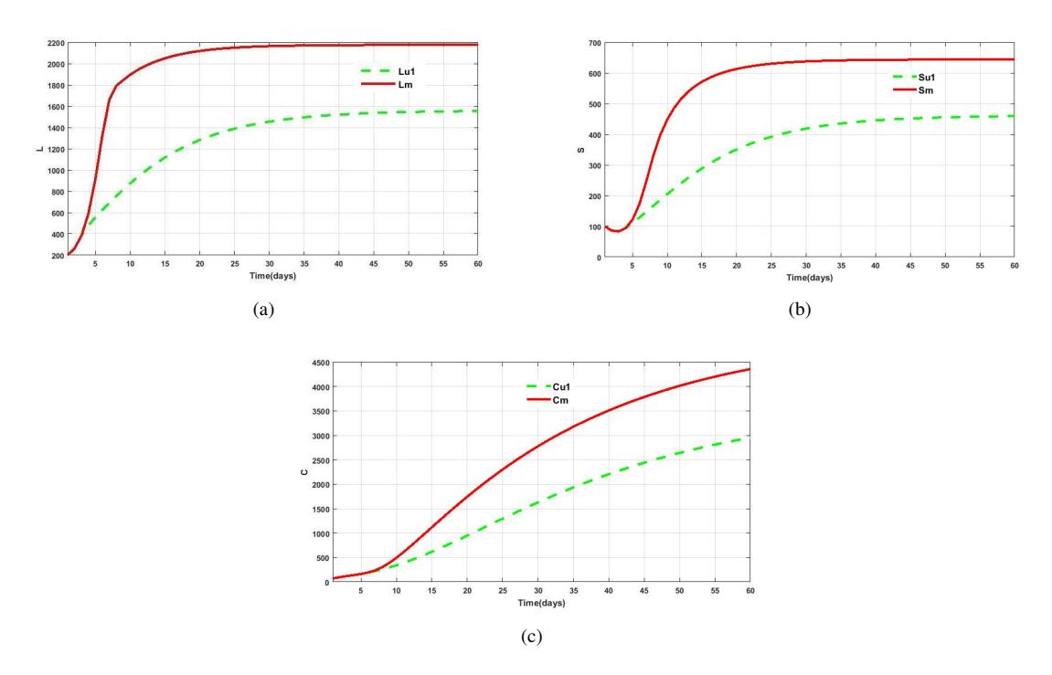
Figure 2: Fast food consumers class with and without control u1.
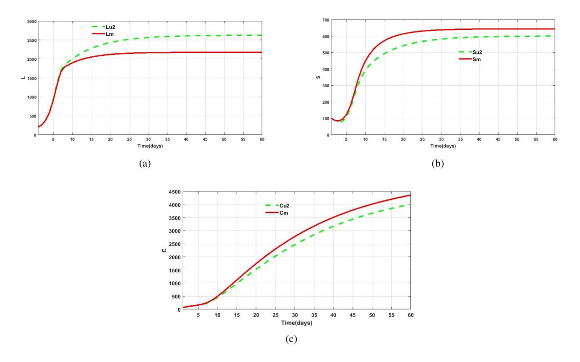
Figure 3: Fast food consumers class with and without control u2.
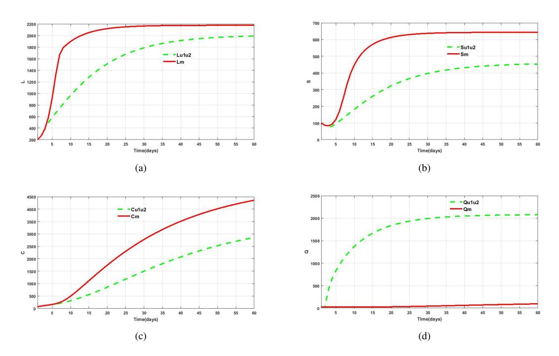
Figure 4: Fast food consumers class with and without controls u1 and u2.
The second objective is to decrease the number of excessive fast food consumers. To achieve this, we exclusively the control u2, i.e., the healthy diet program campaign of the excessive consumers of fast food (see Figures 3). Figure 3b shows a notable reduction in the number of excessive fast food consumers when control measures are applied, compared to a scenario with no control, with the reduction reaching 38% by the end of the chosen control strategy. Figure 3c illustrates that the number of the obese patients decreases from 4400 (C without control u2) to 4000 (C with control u2) at the end of the chosen control. Figure 3a proves that the number of people who stop fast food consumption (without control u2) increases appears under control u2. This increase is not sufficient since the number of people who stop fast food consumption has become moderate consumers of fast food. To improve this situation, we can consider another control corresponding to the obesity treatment for patients.
The third objective is to protect and prevent potential consumers of fast food and the Healthy Diet Program campaign of excessive consumers of fast food. To do this, we utilize the controls u1 and u2, i.e., the unawares program of potential individuals consumers of fast food and the dietary program of excessive consumers of fast food (Figures 4). Figure 4a shows that the number of moderate-income consumers of fast food decreases from 2200 (without control) to 2000 (under control) at the end of the chosen program. The number of excessive fast food consumers decreases from 650 (without control) to 450 (with control) by the end of the adopted control strategy (Figure 4b). We observe in Figure 4c that the obese patient number decreases and reaches 2900 (with control) compared to the scenario without any control, 4400 at the end of the adopted strategy. The number of individuals ceasing fast food consumption rises dramatically from 100 (without controls) to 2100 (with controls) (Figure 4d). This increase indicates the achievement of the objective through the implementation of these controls.
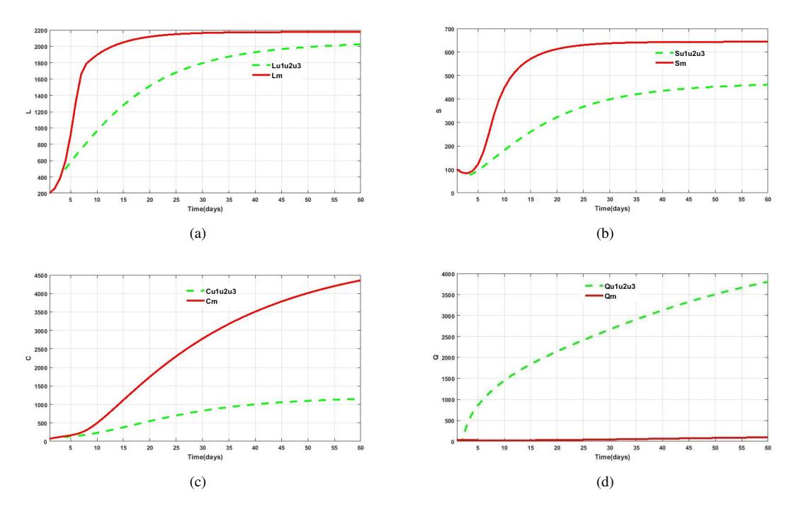
Figure 5: Fast food consumers class with and without controls u1, u2 and u3.
The fourth objective concerns prevention, a Healthy Diet Program campaign for excessive consumers of fast food, and treatment for obesity patients (see Figures 5). To meet this aim, we explore the controls u1, u2, and u3, i.e., awareness programs for the potential individuals consumers of fast food, a healthy diet program campaign for excessive consumers of fast food, and treatment for obesity patients. Hence, we conclude
- Figure 5a shows that the number of moderate individuals consumers of fast food decreases from 2200 (without control) to 2050 (with control) by the end of the applied program.
- Figure 5b shows that the excessive consumer number increases from the early days but then decreases from 650 (without controls) to 475 (under controls).
- Figure 5c shows that the obese patients number increases from the early days but then decreases from 4400 (without controls) to 1100 (under controls).
- Figure 5d illustrates a clear increase in the count of individuals who stop fast food consumption from 100 (without controls) to 3800 (with controls). As a result, the previous objective has been attained.
CONCLUSION
We introduced below a discrete model of fast food consumption with the objective of minimizing the number of excessive consumers and maximizing the number of individuals who stop fast food consumption. The results showed that those awareness programs, healthy diet program campaign and treatment have real influence on of fast food consumption dynamics, and can considerably impact the spread of fast food consumption. We introduced three controls representing awareness programs, encouragement, and follow-up. By applying control theory, we determined the optimal controls. Numerical simulations showed that these control strategies are effective.
ACKNOWLEDGEMENT
The authors thank the reviewer for all the constructive comments.