

1. INTRODUCTION
The oil palm (Elaeis guineensis) is an industrial plant [24]. The cultivation and breeding of oil palm are ruled by specific laws and regulations [29]. Nowadays, oil palm become a strategic commodity. Crude Palm Oil (CPO) is a product of this plant that can be utilized as a renewable energy source [25], [15]. Soh stated that the high demand for palm oil as biofuel and in various products requires efficient production [35]. It triggers a need to increase the production. Increasing oil palm production was driven by many reasons. To improve the characteristics such as heavy bunches, oil yield, oil quality, stress tolerance or adaptability to new environments, and the need for new market niches. Despite those, there is a growing need to explore and develop new varieties with high potential yield and the genetic diversity required to maintain oil palm yield stability [17].
The oil palm has three varieties with different shell thickness characteristics: 1) Dura, 2) Pisifera, and 3) Tenera. Dura has a thick shell. Pisifera is known for having a very slim shell. The Tenera variety is a hybrid breeding between the Dura and Pisifera varieties [2], [36]. Figure 1 illustrates the three varieties of oil palm. Due to the wide range of male and female parental varieties, it would be ideal to breed all these parents to gather comprehensive information on the characteristics of the progeny [2], [36]. However, this task presents significant challenges. Therefore, the researchers employ an experimental method and design to minimize variations in breeding and planting. The Alpha Lattice Design application is widely used for oil palm planting designs [37], [7], [22], [33]. The breeding step applies the Connected Design principle. During its implementation, various obstacles may arise that cause the process and results to deviate from the ideal conditions. Given such circumstances, the challenge lies in determining or selecting the parent palm that can
*Corresponding author
Received May 7th, 2024, Revised July 17th, 2024 (first), Revised October 19th, 2024 (second), Accepted for publication November 28th, 2024. Copyright ©2025 Published by Indonesian Biomathematical Society, e-ISSN: 2549-2896, DOI:10.5614/cbms.2025.8.1.3
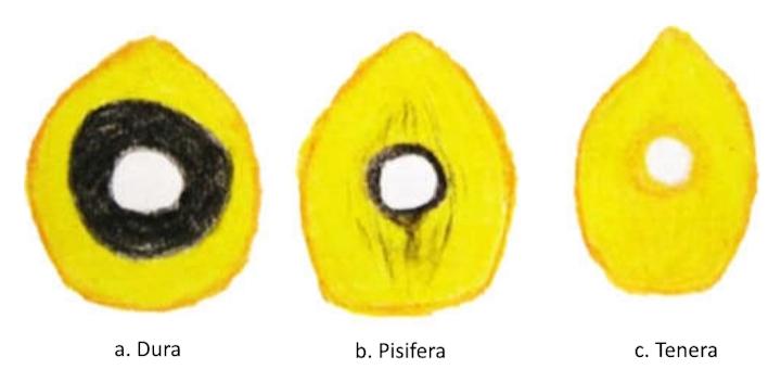
Figure 1: Cross section of the shell of the palm fruit a) Dura, b) Pisifera and c) Tenera.
yield desirable progeny. Breeding between selected female and male parents aimed to determine parents that possess superior characteristics. The female parents are selected from various types of Dura oil palms, while the male parents are from various Pisifera and Tenera oil palms. Concisely, the aim was to determine the value of the phenotype of the progeny [2], [36] and to calculate the ability to transmit parental characteristics to their progeny in subsequent generations. This ability is referred to as General Combining Ability (GCA) and Specific Combining Ability (SCA) in breeding [19].
Quantitative genetic theory explains the process of character inheritance [20]. Quantitative character analysis began with Brownian motion [4]. This analysis was applied to wheat races and commercial cultivars [12] and soybeans [21]. It evaluated the genetic value passed on from the parents to an individual (offspring). Estimation of this genetic value can use phenotype or genomic data. Two components, GCA and SCA, are commonly assessed. GCA is the deviation of an individual's mean value from the population's mean value [18]. The higher the value of this ability, the higher the genetic traits inherited by the parent. SCA results from dominant effect and allele interaction in loci [18]. In other words, the interaction between parents (male and female) has significant value. Estimation can be done in many ways, for example, with a regression model like that done by Fernandez and Miller [10], but the model commonly used today is the Linear Mixed Model (LMM).
In a study by Oliveira et al. [27], mixed models, multivariate analysis, and traditional phenotype selection methods were compared to determine superior maize genotypes in the breeding field. The result was a selection based on the LMM, complemented by multivariate analysis with means, which increased the accuracy of determining the best genotype. In that same year, the same model was used to evaluate and predict the yield of the new wheat genotype [1], demonstrating its stability compared to traditional approaches, where percentage yield determined the genotype performance. Next, Baeza-Rodriguez et al. used a generalized LMM to compare three multiracial population models: the linear animal, the linear sire, and the logistic sire. Their study aimed to evaluate the fertility of heifers on Simmental-Simbrah cattle farms [1]. Specifically in oil palm breeding, Soh used the Best Linear Unbiased Predictor (BLUP) of the LLM in ranking oil palm parents [34]. Likewise, Purba et al. stated that this model helped determine and select the oil palm parents for nurseries [30]. In the past few years, Peixoto et al. have also used this formula for selecting oil palms [28]. Based on the description above, we examine the problems still open for research, including in the multi-site experimental design with repeated measurements. This study is devoted to oil palms where the progenies were planted in two locations. The problem is that the two sets of progenies were inherited from different parents. Hence, the subject under study is the determination of the method of selecting the parent (male and female) of oil palm with the conditions previously mentioned. This study aims to determine the method of oil palm parent selection with certain constraints, as stated in the research problem above. In this case, to link two different sets of progenies, the element of kinship can be used; that is, the closer the kinship, the more genetically similar they are. Therefore, this method will use pedigree information. The next goal is to develop a mathematical model to determine GCA and SCA. We propose the LMM that accommodates the alpha lattice design factors. By accommodating the factors, the model error will be reduced and the likelihood of LMM maximized. In addition to the two general objectives above, we also design specific objectives, namely 1)
exploring the heritability of the oil palm trait, and 2) deepening the model by utilizing pedigree information. After conducting several comparative studies over the years, we observed the potential novelty that this research would bring. It is a method of determining and selecting oil palm parents, calculating combining power values, and predicting progeny and parent values in breeding techniques. The method is LMM with alpha lattice design components as linear terms, including the additive relationship matrix that forms the parent and progeny covariance matrices. This model will benefit the breeder facing the indicated conditions. The paper is organized as follows: 1. Introduction, 2. Data Preparation, 3. Research and Methodology, 4. Result and Discussion, 5. Conclusion, 6. References, and 7. Appendices.
2. DATA PREPARATION (EXPERIMENTAL DATA)
The experiment carried out by the research team followed the Reciprocal Recurrent Selection (RRS) design [8]. This method has been used for genetic improvement [32] and increased Orange-Flashed Sweet potato production [14]. A private incorporation gave access to the experimental data with Non-Disclosure Agreement (NDA) permission. It was collected from Riau in Sumatra and Kumai in Kalimantan, Indonesia (two locations). The data contained three main characteristics. The first was phenotypes. They were the fresh fruit bunch (FFB) of the first three-year productions (FFB1, FFB2, FFB3). FFB is the weight of the oil palm fruit in kg/tree/year. The second was the structure of the experimental design. It consisted of location, replica, block, and plot factors. It constructed an alpha lattice design. The last one was the progenies and their parents. The complete data structure consisted of location, replica, block, progeny, female parent, male parent, FFB1, FFB2, and FFB3 factors. The progeny sets of the two locations are different. No progeny of the same parents was planted in the two locations. The progeny's female parents are Dura. The males are Pisifera and Tenera. Sumatra has 24 Dura, 4 Pisifera, and 9 Tenera varieties. Kalimantan has 19, 2, and 7, respectively. Sumatra has 24 blocks in 4 replicas, 48 plots with 16 same progenies planted on each. Kalimantan has 20 blocks in 4 replicas, 30 plots with 16 same progenies planted on each. The parent selection used third-year production, FFB3. Figure 2 displays the alpha lattice design applied in Kumai.
| 30 | 14 | 21 | 11 | 18 | 5 | 15 | 20 | 10 | 9 | Reg |
|---|---|---|---|---|---|---|---|---|---|---|
| 26 | 23 | 17 | 29 | 19 | 2 | 28 | 22 | 6 | 12 | Replica |
| 1 | 16 | 4 | 24 | 7 | 3 | 27 | 25 | 13 | 8 | | - |
| 12 | 29 | 4 | 22 | 7 | 8 | 9 | 13 | 6 | 17 | Rep |
| 20 | 18 | I 10 | 1 | I 21 | 16 | 1 26 | 3 | l 23 | 19 | Replica II |
| 2 | 30 | l 14 | 5 | l 28 | 15 | l 24 | 25 | l 27 | 11 | | = |
| _ | ||||||||||
| 19 | 14 | 26 | 11 | 10 | 21 | 15 | 24 | 8 | 2 | ζep |
| 19 20 | 14 16 | 26 6 | 11 5 | 10 25 | 21 | 15 27 | 7 | 3 | 17 | Replica I |
| _ | ⊢ i | Replica III | ||||||||
| 20 | 16 | 6 | 5 | 25 | 23 | 7 | 3 | 17 | l _ | |
| 20 13 | 16 | 6 28 | 5 29 | 25 9 | 23 18 | 27 1 | 7 12 | 3 22 | 17 30 | Replica III Replica IV |
Figure 2: Alpha lattice design of plantation in Kumai Kalimantan.
Table 1 shows the snippet of the data. The 3D view of the data of the two locations in Figure 3 illustrates the spread of the data over the replicas and blocks. The statistical description of Sumatra, Kalimantan, and the joined data are displayed in Tables 2, 3, and 4, respectively. Based on those tables, the FFB has an increasing trend. For the joined data, the mean value of the first year is 86.9, 143.6 in the second year (56.7 increase), and 158.3 in the third (14.7 increase). The size of the observation data is 4832. Since there are 36 FFB3 missing values of Sumatra and 26 of Kalimantan, the size reduces to 4770.
Table 1: The snippet of oil palm trial data, that is the fresh fruit bunch of third year yield.
| Trials | Rep | Block | Plot | Progeny | Female | Male | FFB |
|---|---|---|---|---|---|---|---|
| 109.4 | |||||||
| 121 | 110 | 137.5 | |||||
| 203 | 160 | 143.4 | |||||
| Sumatera | 1 | 4 | 142.9 | ||||
| 202 | 168 | 130.3 | |||||
| 147 | 107 | 234.3 | |||||
| 78.2 |
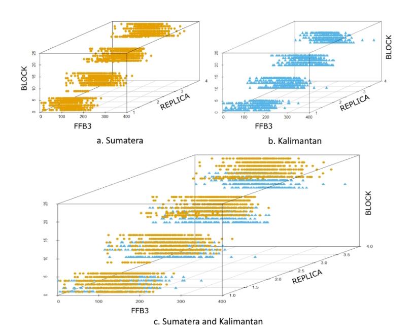
Figure 3: 3D view of the data of the two locations (a) Sumatra (b) Kalimantan and (c) both joined.
Table 2: Descriptive statistics of FFB1, FFB2, FFB3 - Sumatra.
| Phenotype | Min | Q1 | Med | Mean | Q3 | Max | NA's |
|---|---|---|---|---|---|---|---|
| FFB1 | 1.2 | 72 | 97.4 | 96.55 | 122 | 226.8 | 48 |
| FFB2 | 1.5 | 111.2 | 141.8 | 140.9 | 172.7 | 292.9 | 30 |
| FFB3 | 3.3 | 127.6 | 157.7 | 157.1 | 187.5 | 331.1 | 36 |
Table 3: Descriptive statistics of FFB1, FFB2, FFB3 - Kalimantan.
| Phenotype | Min | Q1 | Med | Mean | Q3 | Max | NA's |
|---|---|---|---|---|---|---|---|
| FFB1 | 0.9 | 47.3 | 72.2 | 72.23 | 96.9 | 183.9 | 29 |
| FFB2 | 1.2 | 113.1 | 149.5 | 147.8 | 183.6 | 307.6 | 23 |
| FFB3 | 1.6 | 125.6 | 163.7 | 160.1 | 197.3 | 368.8 | 26 |
Table 4: Descriptive statistics of FFB1, FFB2, FFB3 - Sumatra and Kalimantan.
| Phenotype | Min | Q1 | Med | Mean | Q3 | Max | NA's |
|---|---|---|---|---|---|---|---|
| FFB1 | 0.9 | 61.1 | 87.1 | 86.9 | 113.4 | 226.8 | 77 |
| FFB2 | 1.2 | 112.0 | 144.5 | 143.6 | 176.6 | 307.6 | 53 |
| FFB3 | 1.6 | 126.9 | 160.1 | 158.3 | 191.9 | 368.8 | 62 |
Figure 4 displays the histograms of FFB data and their correlations. The FFB data are from two locations and the three years of observation. Visually, in the first year, the histograms tend to skew left, and for the next two years, they are almost symmetric and normally distributed. The correlation between FFB3 and FFB2 is 0.52, and between FFB3 and FFB1 is 0.43. These correlation values are not high. These show that the production is not mature yet. The production is also still increasing. The LMM analysis will use the phenotype of FFB3.
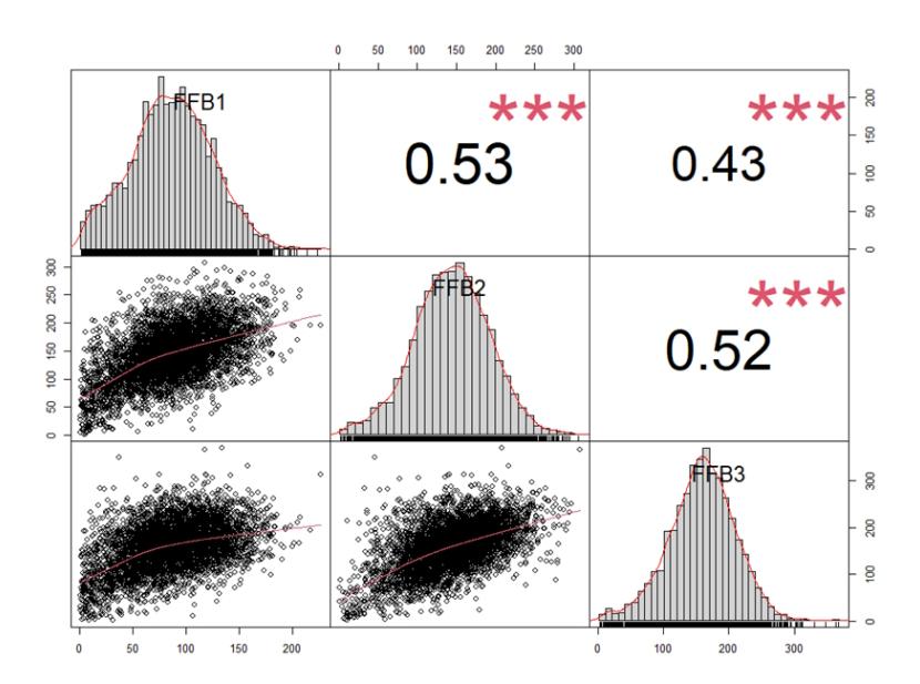
Figure 4: Histogram plots of FFB for the three years of total observation from Sumatera (top), Kalimantan (middle) and both locations (bottom).
3. RESEARCH METHODOLOGY
The Linear Mixed Model was developed by Henderson in 1975 [16] and applied in animal breeding. This model is commonly represented by the following equation.
\[\mathbf{y} = X\beta + Z\nu + \epsilon. \tag{1}\]
In Equation (1), X represents the design matrix of size \(n \times p\), \(\beta\) is a vector of parameters for the fixed effects of size p, Z is an observed random effect design matrix with dimensions \(n \times q\), \(\nu\) is the random effect parameter vector with a size of q and is assumed to be normally distributed with mean 0 and covariance G, and \(\epsilon\) is an unobserved error term that follows a normal distribution with \(E[\epsilon] = 0\) and \(Var[\epsilon] = \sigma_{\epsilon}^2 I\), denoted as \(\epsilon \sim \mathcal{N}0, \sigma_{\epsilon}^2 I\)) with I is an \(n \times n\) identity matrix. The elements of the matrix Z typically take values of 0 and 1.
The structure of the experimental data consists of alpha lattice design components (location, replica, block, and plot) and the genetic factors (male and female parent). Since the two locations are separated (each located on a different island), each replica and associated blocks are assumed to be samples of all possible locations. So, the replicas and blocks are considered random effects. The male, the female, the interaction between the male and female parents, and the interaction between blocks and the progeny are random effects [11]. The only fixed effect is the location.
LMM which accommodates alpha lattice design (the environment), the genetics, and their interaction factors can be represented by Equation (2).
\[\mathbf{y} = X\beta + Z_1 \nu_{Loc:Rep} + Z_2 \nu_{Loc:Rep:Block} + Z_3 \nu_{Loc:Rep:Block:P} + Z_M \nu_M + Z_F \nu_F + Z_{F:M} \nu_{F:M} + \epsilon, \quad (2)\]
where X is the fixed effect design matrix, \(Z_1\), \(Z_2\), \(Z_3\), \(Z_M\), \(Z_F\), and \(Z_{F:M}\) are the design matrices of replicas in location, blocks in replicas in location, the interaction between blocks in replicas in location and progeny, the male, the female, and the progeny factors, respectively. The parameters \(\beta\) is the location fixed effect factor, \(\nu_{Loc:Rep:Blok}\), \(\nu_{Loc:Rep:Blok:P}\), \(\nu_{M}\), \(\nu_{F}\), and \(\nu_{P}\) are the random effects of replicas in location, blocks in replicas in location, the interaction between blocks in replicas in location and progeny, the male, the female, and the progeny factors, respectively, and \(\epsilon\) is the error random effect. Based on the data, the size of each component in Equation (2) is \(y:4770\times1\), \(X:4770\times2\), \(\beta:2\times1\), \(Z_1:4770\times8\), \(\nu_{Loc:Rep:Block}:8\times1\), \(Z_2:4770\times192\), \(\nu_{Loc:Rep:Block}:192\times1\), \(Z_3:4770\times14976\), \(\nu_{Loc:Rep:Block:P}:14976\times1\), \(Z_M:4470\times22\), \(\nu_M:22\times1\), \(\nu_{F:M}:4770\times41\), \(\nu_{F:M}:4770\times78\), \(\nu_{F:M}:78\times1\), \(\epsilon:4770\times1\). The factor of parent interaction effect will be approximated by the progeny effect because the progeny is a result of crossing the parents:
\[\nu_{F\cdot M} \approx \nu_P\].
Each of the random effect factors in Equation (2) is assumed to be normally distributed with mean \(\mathbf{0}\). The distribution of each of them is shown in Equation (3).
\[\nu_{Loc:Rev} \sim \mathcal{N}(\mathbf{0}, G_1), \nu_{Loc:Rev:Block} \sim \mathcal{N}(\mathbf{0}, G_2), \nu_{Loc:Rev:Block:P} \sim \mathcal{N}(\mathbf{0}, G_3),\]
\[\nu_M \sim \mathcal{N}\mathbf{0}, G_M), \nu_F \sim \mathcal{N}\mathbf{0}, G_F), \nu_P \sim \mathcal{N}\mathbf{0}, G_P).\]
The solution of the LMM equation (2) is
\[\hat{\beta} = (X^{t}V^{-1}X)^{-1}X^{t}V^{-1}\mathbf{y}, \hat{\nu} = (Z^{t}\Sigma^{-1}Z + G^{-1})^{-1}Z^{t}\Sigma^{-1}(\mathbf{y} - X\hat{\beta}),\] (3)
where
\[G = \begin{bmatrix} G_1 & 0 & 0 & 0 & 0 & 0 \\ 0 & G_2 & 0 & 0 & 0 & 0 \\ 0 & 0 & G_3 & 0 & 0 & 0 \\ 0 & 0 & 0 & G_M & 0 & 0 \\ 0 & 0 & 0 & 0 & G_F & 0 \\ 0 & 0 & 0 & 0 & 0 & G_P \end{bmatrix}, \quad Var(\mathbf{y}) = V = ZGZ^t + \Sigma,\] and \(G_1, G_2, G_3, G_M, G_F, G_P\) are the covariance matrices of the replicas in location, the blocks in replicas in location, the interaction between blocks in replicas in location and progeny, the male, the female, and the progeny factors, respectively, and \(\Sigma\) is the covariance of error. The solution depends on the variance of random variable y, V.
GCA analysis was performed on data obtained from the two locations. But the progeny sets of two locations did not intersect, no progeny of the same parent was planted in either location. It violated the alpha lattice design principle where all the progenies must be planted on all replicas. This problem can be overcome by linking the two sets with pedigree information. This information is transformed into a coefficient of parentage or additive relationship matrix. The additive relationship is used as a measure of the covariance of breeding
values between relatives. Nilforooshan et al. [26] showed how to calculate this type of matrix. In this analysis, the following assumption is held.
\[G_{1} = \sigma_{1}^{2}I, G_{2} = \sigma_{2}^{2}I, G_{3} = \sigma_{3}^{2}I, G_{M} = \sigma_{M}^{2}A_{M}, G_{F} = \sigma_{F}^{2}A_{F}, G_{P} = \sigma_{P}^{2}A_{P}, \Sigma = \sigma_{\epsilon}^{2}I,\] \[\nu_{Loc:Rep} \sim \mathcal{N}(\mathbf{0}, \sigma_{1}^{2}I), \nu_{Loc:Rep:Block} \sim \mathcal{N}(\mathbf{0}, \sigma_{2}^{2}I), \nu_{Loc:Rep:Block:P} \sim \mathcal{N}(\mathbf{0}, \sigma_{3}^{2}I),\] \[\nu_{M} \sim \mathcal{N}(\mathbf{0}, \sigma_{M}^{2}A_{M}), \nu_{F} \sim \mathcal{N}(\mathbf{0}, \sigma_{M}^{2}A_{F}), \nu_{P} \sim \mathcal{N}(\mathbf{0}, \sigma_{M}^{2}A_{P}),\] where \(A_M, A_F\), and \(A_P\) are the additive relationship matrices of the male parent, the female parent, and the progeny, respectively.
Since the model contains the genetic effects (the male and female parents), we will use the coefficient of parentage (additive relationship matrix) to link the progeny of Sumatra and Kalimantan. We will focus on block matrix
\[\begin{bmatrix} G_M & 0 & 0 \\ 0 & G_F & 0 \\ 0 & 0 & G_P \end{bmatrix}.\]
Define the additive relationship matrices
\[A_M = \begin{bmatrix} A_{M_S} & A_{M_{S:K}} \\ A_{M_{K:S}} & A_{M_K} \end{bmatrix}, \quad A_F = \begin{bmatrix} A_{F_S} & A_{F_{S:K}} \\ A_{F_{K:S}} & A_{F_K} \end{bmatrix}, \quad A_P = \begin{bmatrix} A_{P_S} & A_{P_{S:K}} \\ A_{P_{K:S}} & A_{P_K} \end{bmatrix},\] where \(A_{M_S}\), \(A_{M_K}\), \(A_{F_S}\), \(A_{F_K}\), \(A_{P_S}\), \(A_{P_K}\) are additive relationship matrices of the male parent of Sumatra, the male parent of Kalimantan, the female parent of Sumatra, the female parent of Kalimantan, the progeny of Sumatra, and the progeny of Kalimantan, respectively, \(A_{M_{S:K}}\), \(A_{F_{S:K}}\), and \(A_{P_{S:K}}\) are additive relationship matrices of the male parent of Sumatra and Kalimantan, the female parent of Sumatra and Kalimantan, and the progeny of Sumatra and Kalimantan, respectively. The distribution of \(\nu_M\), \(\nu_F\), and \(\nu_P\) are:
\[\nu_{M} \sim \mathcal{N}(\mathbf{0}, \begin{bmatrix} A_{M_{S}} & A_{M_{S:K}} \\ A_{M_{K:S}} & A_{M_{K}} \end{bmatrix}), \quad \nu_{F} \sim \mathcal{N}(\mathbf{0}, \begin{bmatrix} A_{F_{S}} & A_{F_{S:K}} \\ A_{F_{K:S}} & A_{F_{K}} \end{bmatrix}), \quad \nu_{P} \sim \mathcal{N}(\mathbf{0}, \begin{bmatrix} A_{P_{S}} & A_{P_{S:K}} \\ A_{P_{K:S}} & A_{P_{K}} \end{bmatrix}).\]
Hence, the variance of y is
\[V = [Z_1 Z_2 Z_3 Z_M Z_F Z_P] \begin{bmatrix} \sigma_1^2 I & 0 & 0 & 0 & 0 & 0 & 0 \\ 0 & \sigma_2^2 I & 0 & 0 & 0 & 0 & 0 \\ 0 & 0 & \sigma_3^2 I & 0 & 0 & 0 & 0 \\ 0 & 0 & 0 & \sigma_M^2 A_M & 0 & 0 & 0 \\ 0 & 0 & 0 & 0 & \sigma_F^2 A_F & 0 \\ 0 & 0 & 0 & 0 & 0 & \sigma_P^2 A_P \end{bmatrix} \begin{bmatrix} Z_1^t \\ Z_2^t \\ Z_3^t \\ Z_M^t \\ Z_F^t \\ Z_P^t \end{bmatrix}.\]
Appendix 1 Table 10 lists the pedigree information of the oil palm used in this analysis and Table 11 lists its corresponding additive relationship matrix (snippet).
Several researchers have conducted the oil palm selection for breeding programs, including Purba et al. [30], Soh [35], and Peixoto et al. [28]. Table 5 shows the summary of the differences between this model and theirs. In summary, the model in this analysis focuses on male and female parent selection by treating the replicas, blocks, interaction between blocks and progeny, male and female parent, and progeny as random effects. The aim of accommodating the mentioned factors, is that the parents selected will pass down the character of adaptability to different locations to their offspring. We ran the LMM using the R library Sommer version 4.3.4 [5] [6], and calculated the Additive Relationship matrix using the R library Pedigreemm version 0.3-4 [3]. The R version is 4.3.2 for Windows [31].
| Factor | Soh (1994) | Purba (2001) | Peixoto (2015) | This model (2024) | ||
|---|---|---|---|---|---|---|
| Fixed Effects | Genetic group | Trail | Trail | Location | ||
| Random Effects | Progeny, male parent, female parent | Parent of group A, par ent of group B, interac tion between parent of group A and B | Progeny, male parent, female parent | Replica in location (loc:rep), blocks in loc:rep (loc:rep:block), interaction between loc:rep:block and progeny, male parent, female parent, progeny | ||
| Experimental design | Randomized Block | Randomized Complete Block (mostly) | Randomized Complete Block | Alpha Lattice De sign/Randomized Incomplete Block | ||
| Selection | Male parent | Parent | Family | Male and female parent | ||
Table 5: The differences between the model other previous researches.
4. RESULTS AND DISCUSSION
The variance components of LMM equation (2) are shown in Table 6 and the fixed effect estimations in Table 7. The variance component of female parents is 834.77. It is higher than the male parents which is 51.56. The ratio is about 16.2 times. In inheriting the trait, the female has a higher impact than the male. Although small enough compared to the female, the male effect cannot be neglected [35]. For a female parent, the highest GCA value is 30.23 and the lowest is -59.04 while for the male parent are 5.14 and -4.88, respectively. The location effect estimation values of Sumatra and Kalimantan are 142.0 and 144.4, respectively. They are very close. The heritability value is 0.81 based on Gioia et al. [13]. The value is high. This shows that there is high genetic control for the trait. Parent selection will be advantageous, particularly for the female parent. The first 5 of the highest GCA females are the candidates of superior female parents.
Table 6: Variance components of LMM equation 2.
| Factor | Variance-covariance component |
|---|---|
| Loc:Rep | 35.24 |
| Loc:Rep:Block | 213.34 |
| Loc:Rep:Block:P | 371.93 |
| Progeny | 59.87 |
| Female | 834.77 |
| Male | 51.56 |
| Error | 1807.31 |
Table 7: The Fixed effect estimation values.
| Factors | Estimation value |
|---|---|
| Location 1 | 142.0 |
| Location 2 | 144.4 |
The GCA values of these females are above 25. They are ID 137, 155, 126, 147, and 159. ID 137, 126, and 159 are of Kalimantan and ID 155 and 147 are of Sumatra. The first 4 of the highest GCA are ID 101, 113, 109, and 117. ID 117 is of Kalimantan and the rest are of Sumatra. The GCA values of the parent is displayed in Table 8.
Table 9 shows the average weight of the oil palm bunch of the female and male parents. The selection is reasonable. The selected female parents are among the top 5. For the male parents, 3 of 4 are among the top 5, and only ID 113 is not. This shows that their corresponding progenies' performances are among the top productive yields.
Table 8: GCA values of female and male parents (ordered from largest to smallest).
| ID Female | GCA | ID Female | GCA | ID Male | GCA |
|---|---|---|---|---|---|
| 137 | 30.2378891 | 139 | 15.3943678 | 101 | 5.1399761 |
| 155 | 30.1729883 | 134 | 15.1107185 | 113 | 4.9548271 |
| 126 | 29.3908126 | 151 | 15.0924924 | 109 | 4.9353 |
| 147 | 27.0855274 | 158 | 14.3700068 | 117 | 4.5638783 |
| 159 | 25.9571829 | 149 | 13.6106632 | 100 | 4.2169756 |
| 125 | 23.965404 | 141 | 12.8018348 | 116 | 4.0216417 |
| 128 | 23.5795049 | 157 | 11.7099035 | 114 | 3.9338027 |
| 136 | 22.8887212 | 129 | 11.5627134 | 99 | 3.8246342 |
| 124 | 22.6749783 | 123 | 10.953722 | 115 | 3.5878338 |
| 150 | 22.0557911 | 156 | 10.2557247 | 102 | 2.9622833 |
| 154 | 21.3618275 | 144 | 7.5875052 | 104 | 1.3317078 |
| 148 | 21.158078 | 131 | 7.2298169 | 112 | 0.655304 |
| 127 | 20.1315429 | 133 | 5.8275816 | 108 | -0.4901503 |
| 153 | 19.1152555 | 121 | 4.9835485 | 105 | -0.9552536 |
| 119 | 18.8412355 | 145 | 4.9716269 | 96 | -1.1201911 |
| 142 | 18.1976069 | 118 | 3.1870911 | 111 | -1.403554 |
| 143 | 17.5823985 | 122 | 0.9664901 | 98 | -1.4743577 |
| 152 | 17.0222825 | 132 | 0.5985304 | 107 | -1.5822143 |
| 138 | 16.5874891 | 135 | -5.4666733 | 106 | -1.9428063 |
| 146 | 16.2486114 | 140 | -59.035955 | 110 | -3.7566837 |
| 130 | 15.9270587 | 97 | -4.0268603 | ||
| 103 | -4.8786914 |
Table 9: The 5 highest average FFB values of female and male parent.
| No | Female ID | Progeny Average FFB | Male ID | Progeny Average FFB |
| 1 | 159 | 187.9062 | 117 | 177.0016 |
| 2 | 147 | 186.3766 | 116 | 172.3350 |
| 3 | 137 | 183.2984 | 101 | 171.8451 |
| 4 | 155 | 179.2489 | 100 | 170.5906 |
| 5 | 126 | 177.0012 | 109 | 168.1410 |
There are new crossings between the selected female and male parents that are not on the plantation yet. They are candidates for the new superior seeds. They have the high potential to pass down superior traits to offspring: 1) high oil yield, and 2) ability to adapt to the two locations. For example, the crossing between ID 137 of Kalimantan and ID 101 of Sumatra has the highest total additive genetic value (35.37) among the selected parents. Potentially, all possible crossings between selected female and male parents have these characteristics. This result is beneficial to the breeder and feasible for commercial seeds. Both industry and homeland farmers will have an alternative source of superior seeds. This will minimize the risk of loss because of getting low-production oil palm seeds.
Although the aim is to get the parents whose progeny is adaptable to any location or environment, we performed the analysis using the data from two locations. To make the analysis more robust, more samples from various locations are required. The model might be improved by accommodating the weather, season, soil, and other natural factors. The assumption of no dominant, epistatic, or other genetic effect might be violated, as well. Since the phenotype analyzed was FFB3 (6 years after planting), it might not represent the true productive progeny. The mature productivity of oil palm is in the 8-14 years after planting [23]. Purba et al. [30] use 7-9 years after planting as a mature oil palm tree. Danylo et al. [9] quoted that the oil palm reaches a high mature productivity at the age of 7-15 years after planting.
5. CONCLUSION
Oil palm parents (both female and male) having potential superior genetic characteristics are selected using an LMM. The LMM accommodates the following random effects factors: 1) location, 2) replica, 3) block, 4) interaction between blocks in replicas in location and progeny, 5) female parent, 6) male parent, and 7) progeny. The location is considered a fixed effect. There are two locations in which the sets of their progenies are non-intersect. The model uses pedigree information to link the progenies. This pedigree information contributes to the variance-covariance structure of the LLM. We use the phenotype FFB3 in this analysis. The selected female parents are ID 137, 155, 126, 147, and 159. All of them are Dura varieties. The selected male parents are ID 101, 113, 109, and 117. ID 101 and 117 are Pisifera. The rest are Tenera. The oil palm female parents have a higher impact than the male in inheriting the trait. The variance component of the female parent is greater than that of the male parent. The selection is advantageous for the superior characteristics because the heritability is high. This selection also results in new potential crossings. The crossings will inherit the following traits: 1) a high productive yield and 2) adaptability to different locations.