

1. Introduction
The infectious disease known as tuberculosis (TB) is caused by bacillus Mycobacterium tuberculosis (Mtb), which is dispersed in the air by patients with TB. Although pulmonary tuberculosis is a disease that usually affects the lungs, extrapulmonary TB can also affect other sites. One of the main causes of disease and death globally is tuberculosis (TB). Before the coronavirus (COVID-19) pandemic, TB was the second most common infectious agent-related cause of death, after HIV [40]. Globally, the number of new and relapse cases per 100,000 people annually is decreasing, but not fast enough to meet the first milestone of the End TB Strategy: a 20% decrease in the incidence rate of TB from 2015 to 2020. Globally, between 2015 and 2019, there was a cumulative decrease of 9%, from 142 to 130 new and relapsed cases per 100,000 people. This decrease included a decrease of 2.3% from 2018 to 2019 [8].
The United Nations (UN) Secretary-General's 2020 progress report on tuberculosis (TB) is outlined in the 2020 Global TB Report. This report includes initial evaluations of the potential effects of the 2019 unprecedented coronavirus disease pandemic (COVID-19) on health services, treatment, and efforts to prevent tuberculosis. However, even before the COVID-19 pandemic struck, efforts to control tuberculosis (TB) were not progressing as planned, and there is still a significant discrepancy in the number of TB cases worldwide between estimates and figures provided to public health authorities. Therefore, it cannot be assumed that the failure to meet the target is due to a discrepancy between the estimated and reported numbers of tuberculosis cases. Of the 10 million individuals who were thought to have contracted tuberculosis in 2019, 7.1 million
*Corresponding author
Received December 13<sup>th</sup>, 2023, Revised October 24<sup>th</sup>, 2024, Accepted for publication June 20<sup>th</sup>, 2025. Copyright ©2025 Published by Indonesian Biomathematical Society, e-ISSN: 2549-2896, DOI:10.5614/cbms.2025.8.1.8
(71%) were found and reported to national TB programs worldwide; the remaining 2.9 million individuals (29%) were not included in this figure. Those who were diagnosed with tuberculosis (TB) but did not report their condition to the private sector or public health authorities, as well as those who were not diagnosed and therefore did not receive treatment, are among the missing individuals with TB [8].
An estimated 10.0 million people worldwide contracted TB in 2019, accounting for 1.2 million TB-related deaths among HIV-negative individuals and an additional 208,000 deaths among HIV-positive individuals. People of all ages and genders are affected by tuberculosis (TB), but adult males bear the greatest burden: They make up 56% of all cases, compared to 32% for adult women and 12% for children under the age of 15. 8.2% of all TB cases involved HIV-positive individuals. Geographically, the WHO regions of South East Asia (44%), Africa (25%), and the Western Pacific (18%) had the highest percentages of tuberculosis cases in 2019. The Eastern Mediterranean (8.2%), the Americas (2.9%), and Europe (2.5%) had the lowest percentages. Twothirds of the total worldwide was made up of eight countries: South Africa (3.6%), Nigeria (4.4%), Bangladesh (3.6%), India (26%), Indonesia (8.5%), China (8.4%), Philippines (6.0%), Pakistan (5.7%), Nigeria (4.4%) and Bangladesh (3.5%) [8].
Inhalation of Mtb organisms is the first step in the natural history of tuberculosis. After a time of bacterial propagation and replication, live bacilli are immunologically contained. Asymptomatic latent tuberculosis infection is the result of this process [18]. According to a 2016 global modeling study, roughly 1.7 billion people were latently infected with Mtb, representing around 25% of the global population [21]. There is strong evidence that Mtb infection can self-clear, and recent analyses and commentary point to a lower number of people currently infected [15]. Most people with immunoreactivity to tuberculosis can manage their infection and do not progress to active tuberculosis when immunosuppressed, meaning they cannot spread the disease. This suggests that they have successfully cleared their infection while still having an immunological memory of it [4]. People with HIV and those exposed to risk factors such as alcohol consumption, smoking, diabetes, and undernourishment have a significantly higher chance of developing tuberculosis (TB) disease [40].
When Mtb enters the alveolar air sacs of the lungs, the primary infection of tuberculosis (TB) starts when the pathogen invades and replicates inside the endosomes of alveolar macrophages. Although macrophages are known to be pathogen-killing professionals, Mtb has developed amazing strategies to avoid host defenses and create the ideal environment for survival and proliferation [42]. In addition to the formation of granulomas, macrophages and CD4 + T lymphocytes have long been considered the cornerstones of the immune response against Mtb, and their importance is evident [12]. Granulomas are central to the immunopathogenesis of tuberculosis because they are a characteristic of Mtb infection. Reactivation of a granuloma that has already formed in a latently infected individual or early progression of the primary granuloma during the infection process can lead to tuberculosis. Granulomas are well-organized and dynamic structures that arise at the location of bacteria and are mediated during the infection process by particular immune responses. The primary function of the granuloma is to confine and localize Mtb while focusing the immune response in a specific area [19].
When inhaled Mtb is consumed and spreads through the alveolar epithelium into lung tissue and surrounding lymph nodes, as well as through the lymphatics and bloodstream, granuloma formation in human pulmonary tuberculosis begins shortly after infection. More mononuclear leukocytes are drawn to the infection site as a result of the immune response that is triggered, which also activates phagocyte antimicrobial activities. Aggregation of cells surrounding the foci of infected cells results in the granuloma, a mass of cells rich in macrophages. Immune cells in varying stages of differentiation make up a granuloma, with infected macrophages at the center of the accumulation of cells. To control the mycobacterial load in infected cells and activate cytotoxic T cells, recruited T cells secrete cytokines. The cellular makeup of granulomatous TB lesions is made up of B and T lymphocytes, fibroblasts, foamy macrophages, epithelioid cells (a special type of differentiated macrophage), blood-derived infected and uninfected macrophages, and multinucleated giant cells (also known as Langerhans cells) [19].
Mtb is a facultative intracellular pathogen that lives in monocytes [7]. Most infected people have a successful and defensive cell-mediated response and do not experience active disease. Most Mtb infections are manageable (not curable) and enter a latent state. Others experience a short-term (primary infection) or longterm (reactivation) onset of active disease [36]. The usefulness of an experimental model of mycobacterial persistence for methods in identifying underlying mechanisms related to clinical latency, to direct clinical evaluation of new interventions, novel diagnostics, and medications, as well as for the detection, treatment and prevention of disease [4].
Many theoretical investigations have been conducted to comprehend the data on Mtb infection, from immunological and epidemiological perspectives. Different mathematical models, such as [1], [2], [11], [23], [28], [29], [32], [34], [39], [41], [43], [45], [46], [50], have been proposed to evaluate the influence of factors such as Mtb population dynamics, immune system, treatment, and bacterial resistance on the progression of infection.
Specifically, in this work we suggest a model to assess how Mtb growth affects the course of infection. In this model, the earlier research presented in [27], [22], [24], [25], [26] is continued.
2. MODEL FORMULATION
An important factor in how a Mtb infection turns out is the cell-mediated response. A particular immune response triggered by macrophages, T cells, and the cytokines they produce results in the formation of a granuloma at the site of bacteria's implantation. Using the population of uninfected macrophages, infected macrophages, activated macrophages, Mtb bacteria, and T cells - represented by the variables \(M_1\), \(M_2\), \(M_3\), B and T, respectively. We develop a mathematical model for the cell-mediated response against tuberculosis. The ranges and units of the parameters are shown in Table 1.
Resting or uninfected macrophages \((M_1)\) are normally present in the lung [10]. Macrophages have a natural turnover due to monocyte differentiation at a constant rate \(s_1\) and the natural death of cells at a constant rate per capita \(d_1\). We assume that all incoming macrophage cells are equally uninfected \(M_1\) and differentiated because they undergo infection \(M_2\) and activation \(M_3\). In response to chemokines released by activated and infected macrophages, more uninfected macrophages are drawn to the lung infection site when bacteria are present. The macrophage population should remain at \(M_1 = s_1/d_1\), the equilibrium value, in the absence of infection. Uninfected macrophages experience three distinct dynamics during infection: increased recruitment, infection, and activation. At a maximum rate of \(\beta\), uninfected macrophages that cannot eliminate their bacterial load may develop a chronic infection [30]. It is possible to formulate the differential equation for the concentration of uninfected macrophages as
\[\frac{dM_1}{dt} = s_1 - d_1 M_1 - \beta B M_1. \tag{1}\]
The accumulation of infected macrophages leads to the development of the adaptive immune response against Mtb. Briefly, a type 1 T helper \((T_h)\) or CD4<sup>+</sup> T cells immune response and produce IFN-\(\gamma\) to activate bactericidal effector mechanisms of infected macrophages [17]. Additional types of T cells also contribute to the immune response against M.tb infection, including CD8<sup>+</sup> T cells \((T_c)\). CD8<sup>+</sup> T cells are important to induce cytotoxic activity in response kill infected macrophages to control of Mtb infection [19], [33], [48].
Chronic infection results in either infected macrophage killing or natural death (at rate \(d_2\) and \(d_2 \ge d_1\)). Bacteria that reside intracellularly in infected macrophage cells \((M_2)\) will continue to replicate in the cell. Infected macrophage cells \((M_2)\) that cannot accommodate the number of bacteria in the cell will rupture with a rate of cell rupture due to intracellular bacteria at maximal rate \(\mu_2\). Both apoptosis and cytotoxic activity are due to \(CD4^+\) or \(T_h\) cells and \(CD8^+\) or \(T_c\) cells. Infected macrophages grow at a rate \(\beta BM_1\) and are eliminated by \(CD4^+\) or \(T_h\) for macrophage activation, occurring at a rate of \(\alpha_1\). Furthermore infected macrophages are eliminated via cytotoxic activity by \(CD8^+\) or \(T_c\) cells, at a rate of \(\alpha_2\). T cells arrive at the site of infection as fully differentiated \(T_h\) and \(T_c\). p is the proportion of differentiated T cells, \(T_h = pT\) and \(T_c = (1-p)T\). T cells is given by \(T = T_h + T_c\). The differential equation for infected macrophage concentration becomes:
\[\frac{dM_2}{dt} = \beta BM_1 - (\alpha_1 pT + \alpha_2 (1-p)T)M_2 - d_2 M_2 - \mu_2 M_2. \tag{2}\]
Although bacteria are enough to cause infection, IFN-\(\gamma\) is necessary to activate macrophages, which happens at a maximum rate of \(\alpha_1\) [16]. The rate at which activated macrophages naturally die is \(d_3\). The differential equation for the concentration of activated macrophages is provided by
\[\frac{dM_3}{dt} = \alpha_1 pT M_2 - d_3 M_3. \tag{3}\]
Immune cells (T) that have differentiated will migrate to the site of infection through the blood and lymph nodes [30]. Afterward, chemotactic signals from infected macrophages attract immune cells to the infection site [6]. With a proportionality constant \(\gamma\), the recruitment of T cells is inversely correlated with the number of infected macrophages, and their death occurs at a constant rate per capita \(d_4\). Here we obtain the T dynamics formula:
\[\frac{dT}{dt} = s_4 + \gamma M_2 T - d_4 T. \tag{4}\]
The growth rate of extracellular bacteria (B) is r due to self-replication, and their natural death rate is \(d_5\) per capita. We assume that each macrophage has a bacterial carrying capacity of N. An infected macrophage's intracellular bacterial load builds up until it reaches a breaking point, at which point the macrophage bursts. Hence, we get \(N\mu_2M_2\) as the representation of the number of new extracellular bacteria due to the bursting of infected macrophages at a rate of \(\mu_2\). At a rate \(k_1\), extracellular bacteria infect macrophages or are consumed and eliminated by uninfected macrophages. Activated macrophages also kill them at a rate \(k_3\) [36], [50]. In total, we obtain the dynamics formula of B.
\[\frac{dB}{dt} = rB - d_5B - (k_1M_1 + k_3M_3)B + N\mu_2M_2.\] (5)
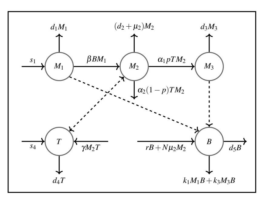
Figure 1: The flow chart for bacteria, T cells, and macrophages.
The flow diagram of bacteria, T cells, and macrophages as described by the differential equations (1)-(5) is shown in Figure 1. The interactions and intracellular growth of these three populations have been visualized by figures and videos in [35]. There are several videos such as macrophage internalization of Mtb aggregates, death of an Mtb-infected macrophage, pyroptotic death of macrophages, Mtb grows inside a dead macrophage treated with IFNy prior to infection and cell death cascade following phagocytosis of a dead infected macrophage in that article. The following system of nonlinear differential equations is satisfied by the model for the development of Mycobacterium tuberculosis infection in the lungs, which is derived from
Equations (1)-(5).
\[\frac{dM_1}{dt} = s_1 - d_1 M_1 - \beta B M_1, \frac{dM_2}{dt} = \beta B M_1 - (\alpha_1 p + \alpha_2 (1 - p)) T M_2 - d_2 M_2 - \mu_2 M_2, \frac{dM_3}{dt} = \alpha_1 p T M_2 - d_3 M_3, \frac{dT}{dt} = s_4 + \gamma M_2 T - d_4 T, \frac{dB}{dt} = r B - d_5 B - (k_1 M_1 + k_3 M_3) B + N \mu_2 M_2.\] (6)
The existence and uniqueness conditions of the system (6) are easily verified. In addition, the designated biological interest region is provided by
\[\Omega = \left\{ (M_1, M_2, M_3, T, B)^T \in \mathbb{R}^5_+ : M_1 \ge 0, M_2 \ge 0, M_3 \ge 0, T \ge 0, B \ge 0 \right\}. \tag{7}\]
We show that all solutions with initial conditions in \(\Omega\) stay there for all \(t \ge 0\) and have biological meaning. First, we introduce the following lemma.
Lemma 2.1. [51] Suppose \(\Omega \subset \mathbb{R} \times \mathbb{C}^n\) is open, \(f_i \in C(\Omega, \mathbb{R}), i = 1, 2, 3, ..., n\). If \(f_i|_{x_i(t)=0, X_t \in \mathbb{C}^n_{+0}} \geq 0, X_t = (x_{1t}, x_{2t}, ..., x_{nt})^T, i = 1, 2, 3, ..., n\), then \(\mathbb{C}^n_{+0}\) is the invariant domain of the following equations
\[\frac{dx_i(t)}{dt} = f_i(t, X_t), t \ge 0, i = 1, 2, ..., n.\]
Theorem 2.2. Each solution in System (6) with nonnegative initial conditions is nonnegative for all t > 0.
Proof: Let \(X = (M_1, M_2, M_3, T, B)^T\) and \(f(X) = (f_1(X), f_2(X), f_3(X), f_4(X), f_5(X))^T\) then we can rewrite System (6) as \(\dot{X} = f(X)\) where
\[f(X) = \begin{pmatrix} f_1(X) \\ f_2(X) \\ f_3(X) \\ f_4(X) \\ f_5(X) \end{pmatrix} = \begin{pmatrix} s_1 - d_1M_1 - \beta BM_1 \\ \beta BM_1 - (\alpha_1 p + \alpha_2(1-p))TM_2 - d_2M_2 - \mu_2M_2 \\ \alpha_1 pTM_2 - d_3M_3 \\ s_4 + \gamma M_2T - d_4T \\ rB - d_5B - (k_1M_1 + k_3M_3)B + N\mu_2M_2 \end{pmatrix}.\]
We can easily confirmed that \(\left. \frac{dM_1}{dt} \right|_{M_1=0} = s_1 \ge 0\), \(\left. \frac{dM_2}{dt} \right|_{M_2=0} = \beta B M_1 \ge 0\), \(\left. \frac{dM_3}{dt} \right|_{M_3=0} = \alpha_1 p T M_2 \ge 0\), \(\left. \frac{dT}{dt} \right|_{T=0} = \alpha_1 p T M_2 \ge 0\).
\(s_4 \ge 0\), \(\frac{dB}{dt}\Big|_{B=0} = N\mu_2 M_2 \ge 0\). Then it follows from Lemma 2.1 that \(\mathbb{R}^5_+\) is invariant set. Subsequently, the solutions with initial conditions in \(\Omega\) remain there for all t > 0.
3. MODEL ANALYSIS
The following algebraic system solutions provide the equilibrium states of the system (6).
\[s_{1} - d_{1}M_{1} - \beta BM_{1} = 0,\] \[\beta BM_{1} - (\alpha_{1}p + \alpha_{2}(1-p))TM_{2} - d_{2}M_{2} - \mu_{2}M_{2} = 0,\] \[\alpha_{1}pTM_{2} - d_{3}M_{3} = 0,\] \[s_{4} + \gamma M_{2}T - d_{4}T = 0,\] \[rB - d_{5}B - (k_{1}M_{1} + k_{3}M_{3})B + N\mu_{2}M_{2} = 0.\] (8)
The solutions of the system (8) indicate the existence of an infection-free equilibrium, \(E_0 = \left(\frac{s_1}{d_1}, 0, 0, \frac{s_4}{d_4}, 0\right)\) and infected compartments, \(M_2\) and B, in which naive T cells control infection. The reproduction number
can be derived by identifying the infection terms and the transition terms of the compartments, as in Van den Driessche and Watmough [49]. Therefore, we obtained the matrices F and V as follows.
\[F = \begin{bmatrix} 0 & \frac{\beta s_1}{d_1} \\ 0 & 0 \end{bmatrix} \text{ and } V = \begin{bmatrix} \sigma & 0 \\ -N\mu_2 & \sigma_1 \end{bmatrix}, \tag{9}\] with
\[\sigma = d_2 + \mu_2 + \frac{s_4(\alpha_1 p + \alpha_2 (1 - p))}{d_4}.\] \[\sigma_1 = -r + d_5 + \frac{k_1 s_1}{d_1}.\] (10)
The eigenvalues that dominate \(FV^{-1}\) are defined in the following Equation (11).
\[R_0 = \frac{\beta s_1 N \mu_2}{d_1 \sigma \sigma_1}.\tag{11}\]
The number of secondary (latent) infections caused by a single infectious particle (bacteria) throughout the mean infectious period is denoted by \(R_0\). The endemic equilibrium in which Mtb infection endures. Regarding \(E_1 = (M_U^*, M_I^*, M_A^*, T^*, B^*)\), the endemic equilibrium. We begin by solving \(M_U^*\), \(M_A^*\), and \(T^*\) from the first, third, and fourth equations of (8) to determine this equilibrium:
\[M_U^* = \frac{s_1}{\beta B^* + d_1}, M_A^* = \frac{\alpha_1 p M_I^* s_4}{(d_4 - \gamma M_I^*) d_3} \text{ and } T^* = \frac{s_4}{d_4 - \gamma M_I^*}.\] (12)
In the second equation of (8), if we substitute \(M_U^*\) and \(T^*\) defined by (12), we obtain
\[\frac{\beta B^* s_1}{\beta B^* + d_1} + \left(\frac{s_4(\alpha_1 p + \alpha_2 (1 - p)) M_2^*}{d_4 - \gamma M_I^*}\right) - (d_2 + \mu_2) M_2^* = 0.\] (13)
We derive the following quadratic equation from (13).
\[M_I^{*2} - b_1(B^*)M_I^* + c_1(B^*) = 0,\] (14)
where
\[b_{1}(B^{*}) = \frac{\beta(\sigma d_{4} + \gamma s_{1})B^{*} + \sigma d_{1}d_{4}}{\gamma(d_{2} + \mu_{2})(\beta B^{*} + d_{1})},\] \[c_{1}(B^{*}) = \frac{\beta s_{1}d_{4}B^{*}}{\gamma(d_{2} + \mu_{2})(\beta B^{*} + d_{1})}.\] (15)
Solution of (14) is
\[M_I^* = f_1(B^*) = \frac{b_1(B^*) \pm \sqrt{[b_1(B^*)]^2 - 4c_1(B^*)}}{2}.\] (16)
Currently, we can solve for \(M_I^*\) by substituting \(M_U^*\) and \(M_A^*\) defined in (12) in the fifth equation of (8).
\[B^* \left( r - d_5 - \frac{s_1 k_1}{\beta B^* + d_1} - \frac{s_4 k_3 \alpha_1 p M_I^*}{(d_4 - \gamma M_I^*) d_3} \right) + N \mu_2 M_I^* = 0.\] (17)
We derive the following quadratic equation from (17).
\[M_I^{*2} + b_2(B^*)M_I^* - c_2(B^*) = 0,\] (18)
where
\[b_{2}(B^{*}) = \frac{\beta (s_{4}\alpha_{1}pk_{3} + \gamma d_{3}(r - d_{5}))B^{*2} + (-\beta Nd_{3}d_{4}\mu_{2} + \alpha_{1}pk_{3}d_{1}s_{4} - \gamma\sigma_{1}d_{1}d_{3})B^{*} - Nd_{1}d_{3}d_{4}\mu_{2}}{N\gamma d_{3}\mu_{2}(\beta B^{*} + d_{1})}.\] \[c_{2}(B^{*}) = \frac{d_{4}B^{*}(\beta B^{*}(r - d_{5}) - \sigma_{1}d_{1})}{N\gamma\mu_{2}(\beta B^{*} + d_{1})},\] (19)
Solution of (18) is
\[M_I^* = f_2(B^*) = \frac{-b_2(B^*) \pm \sqrt{[b_2(B^*)]^2 + 4c_2(B^*)}}{2}.\] (20)
It is important to study the intersections of the aforementioned functions to determine the intersections of the functions (14) and (18). Based on our observation, \(f_1\) and \(f_2\) represent two different expressions for \(M_I^*\) and \(B^*\). We find that the solutions of the functions (14) and (18) are
\[f_1(B^*) = \frac{b_1(B^*) \pm \sqrt{[b_1(B^*)]^2 - 4c_1(B^*)}}{2},\] \[f_2(B^*) = \frac{-b_2(B^*) \pm \sqrt{[b_2(B^*)]^2 + 4c_2(B^*)}}{2}.\] (21)
As \(f_1\) defined in (14) is positive, strictly increasing, and concave, we also obtain that \(f_1(0) = f_2(0)\) from (21). Some obvious properties of \(f_1\) and \(f_2\) are established by the following theorem.
Theorem 3.1. In \(B^* = 0\), the functions \(f_1\) and \(f_2\) intersect. Furthermore, \(f_1\) is concave in the first quadrant, strictly increasing, and positive.
Proof: The roots of the quadratic equation \(f_1(0)\) are \(M_I^{f_1^-}=0\) and the roots of the quadratic equation \(f_2(0)\) are \(M_I^{f_2^-}=0\) and
\[\begin{split} M_{I}^{f_{1}^{+}} &= \frac{b_{1}(B^{*}) + \sqrt{[b_{1}(B^{*})]^{2} - 4c_{1}(B^{*})}}{2} \\ &= \frac{d_{4}\sigma}{\gamma(d_{2} + \mu_{2})} = \frac{d_{4}}{\gamma} \left( 1 + \frac{s_{4}(\alpha_{1}p + \alpha_{2}(1 - p))}{d_{4}(d_{2} + \mu_{2})} \right), \\ M_{I}^{f_{2}^{+}} &= \frac{-b_{2}(B^{*}) + \sqrt{[b_{2}(B^{*})]^{2} + 4c_{2}(B^{*})}}{2} \\ &= \frac{d_{4}}{\gamma}. \end{split} \tag{22}\]
Furthermore, we see that the derivatives of \(f_1\) and \(f_2\) are given by
\[\bar{f}'_1(B^*) = \frac{1}{2} \left[ b'_1(B^*) \pm \frac{b_1(B^*)b'_1(B^*) - 2c'_1(B^*)}{\sqrt{b_1(B^*)^2 - 4c_1(B^*)}} \right], \tag{23}\]
where
\[b'_{1}(B^{*}) = \frac{\beta s_{1}d_{1}}{(d_{2} + \mu_{2})(\beta B^{*} + d_{1})^{2}},\] \[c'_{1}(B^{*}) = \frac{\beta s_{1}d_{1}d_{4}}{\gamma(d_{2} + \mu_{2})(\beta B^{*} + d_{1})^{2}},\] (24)
\[\bar{f}_2'(B^*) = \frac{1}{2} \left[ -b_2'(B^*) \pm \frac{b_2(B^*)b_2'(B^*) + 2c_2'(B^*)}{\sqrt{b_2(B^*)^2 + 4c_2(B^*)}} \right], \tag{25}\]
\[b_{2}'(B^{*}) = \frac{pS_{T}\alpha_{1}k_{A}(\beta B + d_{U})^{2} + B\beta \gamma d_{A}(r - d_{B})(\beta B + 2d_{U}) - \gamma \sigma_{1} d_{U}^{2} d_{A}}{N\gamma d_{A}\mu_{I}(\beta B^{*} + d_{U})^{2}},\] \[c_{2}'(B^{*}) = \frac{d_{T}(\beta B(r - d_{B})(\beta B + 2d_{U}) - \sigma_{1} d_{U})}{N\gamma \mu_{I}(\beta B^{*} + d_{U})^{2}}.\] (26)
From Equations (23) and (25), we obtain
\[f'_{1}(0)^{-} = \frac{\beta s_{1}}{\sigma d_{1}},\] \[f'_{1}(0)^{+} = \frac{s_{1}s_{4}(\alpha_{1}p + \alpha_{2}(1-p))\beta}{d_{1}d_{4}(d_{2} + \mu_{2})\sigma},\] \[f'_{2}(0)^{-} = \frac{\sigma_{1}}{N\mu_{2}},\] \[f'_{2}(0)^{+} = -\frac{p\alpha_{1}k_{3}s_{4}}{N\gamma d_{3}\mu_{2}}.\] (27)
Observe that
\[f_1'(0)^- - f_2'(0)^- = \frac{\beta s_1}{\sigma d_1} - \frac{\sigma_1}{N\mu_2}\] \[= \frac{\sigma_1(R_0 - 1)}{N\mu_2}.\] (28)
From Equation (13), we can also see the derivative of \(B^* = h(M_L^*)\) as follows
\[h'(M_I^*) = \frac{d_1 s_1 \left( (d_2 + \mu_2) (d_4 - \gamma M_I^*)^2 + (\alpha_1 p + \alpha_2 (1 - p)) d_4 s_4 \right)}{\beta \left( \gamma M_I^{*2} (d_2 + \mu_2) + s_U \left( d_4 - \gamma M_I^* \right) - \sigma M_I^* d_4 \right)^2}.\]
Because \(h'(M_I^*) > 0\), \(h(M_I^*)\) increases for \(M_I^* > 0\). Based on the inverse function theorem, \(M_I^* = f_1(B^*)\) is also differentiable and increasing. We compute second-order continuous partial derivatives to evaluate concavity [3]. The Hessian matrix \(f_1\) from (13) is given by
\[H(B^*, M_I^*) = \begin{bmatrix} \frac{\partial^2 f_1}{\partial B^{*2}} & \frac{\partial^2 f_1}{\partial B^{*2}} & \frac{\partial^2 f_1}{\partial B^* \partial M_I^*} \\ \frac{\partial^2 f_1}{\partial M_I^* \partial B^*} & \frac{\partial^2 f_1}{\partial M_I^{*2}} \end{bmatrix} = \begin{bmatrix} 0 & -a \\ -a & -2\gamma(d_2 + \mu_2)(\beta B^* + d_1) \end{bmatrix}, \tag{29}\]
with
\[a = \beta \left( \gamma \left( 2M_I^* \left( d_2 + \mu_2 \right) - s_U \right) - d_4 \sigma \right).\]
From Equation (29), we obtain
\[|0| = 0, \begin{vmatrix} 0 & -a \\ -a & -2\gamma(d_2 + \mu_2)(\beta B^* + d_1) \end{vmatrix} = -a^2.\]
The matrix H is semidefinite negative, since the determinants H are negative and zero. The theorem in [3], [38] can be used to show that \(f_1\) is concave.
We examine two scenarios, \(R_0 < 1\) and \(R_0 > 1\), to assess the presence of endemic equilibrium. In the first instance, the outcome is as follows:
Theorem 3.2. If \(R_0 > 1\), there exists a unique endemic equilibrium.
Proof: First, assume \(R_0 > 1\). We can observe from (22) that in this instance, \(M_I^{f_2^-} = 0\) is satisfied by the roots of \(f_2(0)\). In the first quadrant, \(f_1\) is concave and \(f_2\) is convex, \(f_1'(0) > 0\), \(f_2'(0)^- > 0\), and \(\lim_{B^* \to \infty} f_1(B^*) > 0\) are also satisfied by the roots of \(f_1(0)\). All these conditions implied that \(f_1\) and \(f_2\) only cross once in the positive quadrant. For \(R_0 > 1\) we have
\[f_1'(0)^- - f_2'(0)^- = \frac{\sigma_1(R_0 - 1)}{Nu_2} > 0.\]
Theorem 3.3. Assume \(R_0 > 0\) so that \(\sigma_1 = -r + d_5 + \frac{k_1 s_1}{d_1} > 0\) then
- 1) There is no endemic equilibrium if \(R_0 < 1\) because \(f_1\) and \(f_2\) do not positively intersect.
- 2) There is only one endemic equilibrium for \(f_1\) and \(f_2\) if \(R_0 > 1\). This is because they have only one positive intersection.
This suggests outcomes that are comparable to those found in Theorem 3.2.
3.1. Stability analysis of equilibrium
Conditions for the stability of the equilibrium points are examined in this section. The eigenvalues concerning the system's Jacobian (6), assessed at the equilibrium points, are determined in this way:
\[J \begin{bmatrix} M_1 \\ M_2 \\ M_3 \\ T \\ B \end{bmatrix} = \begin{bmatrix} -(d_1 + \beta B) & 0 & 0 & 0 & -\beta M_1 \\ \beta B & -a_0 & 0 & -a_1 & \beta M_1 \\ 0 & \alpha_1 p T & -d_3 & \alpha_1 p M_2 & 0 \\ 0 & \gamma T & 0 & -(d_4 - \gamma M_2) & 0 \\ -k_1 B & N\mu_2 & -k_3 B & 0 & -a_2 \end{bmatrix},\](30)
where,
\[a_{0} = (\alpha_{1}p + \alpha_{2}(1-p))T + d_{2} + \mu_{2},\] \[a_{1} = (\alpha_{1}p + \alpha_{2}(1-p))M_{2},\] \[a_{2} = k_{1}M_{1} + k_{3}M_{3} - r + d_{5}.\] (31)
For the infection-free equilibrium \(E_0 = (\frac{s_1}{d_1}, 0, 0, \frac{s_4}{d_4}, 0)\), the Jacobian is given by
\[J(E_0) = \begin{bmatrix} -d_1 & 0 & 0 & 0 & \frac{-\beta s_1}{d_1} \\ 0 & -\sigma & 0 & 0 & \frac{\beta s_1}{d_1} \\ 0 & \frac{\alpha_1 p s_4}{d_4} & -d_3 & 0 & 0 \\ 0 & \frac{\gamma s_4}{d_4} & 0 & -d_4 & 0 \\ 0 & N\mu_2 & 0 & 0 & -\sigma_1 \end{bmatrix}.\] (32)
Easy computations reveal that the roots of the quadratic equation and \(\lambda_1 = -d_1\), \(\lambda_2 = -d_3\), and \(\lambda_3 = -d_4\) provide the eigenvalues.
\[\lambda^2 + (\sigma + \sigma_1)\lambda + \sigma\sigma_1(1 - R_0) = 0. \tag{33}\]
The Routh-Hurwitz criterion leads us to the conclusion that if and only if \(R_0 < 1\), then all of the eigenvalues of the equation (33) have negative real parts.
Theorem 3.4. The infection-free equilibrium \(E_0 = (1,0,0,1,0)\) is locally asymptotically stable if \(R_0 < 1\), and unstable when \(R_0 > 1\).
We now examine the stability of the endemic equilibrium, which indicates the persistence of the infection. Following the equilibrium equations (8), we obtain the following equalities.
\[\frac{\frac{s_1}{M_1}}{\frac{BBM_1}{M_2}} = d_1 + \beta B,\] \[\frac{\beta BM_1}{M_2} = (\alpha_1 p + \alpha_2 (1 - p))T + d_2 + \mu_2,\] \[\frac{\frac{s_4}{T}}{T} = d_4 - \gamma M_2,\] \[\frac{N\mu_2 M_2}{B} = (k_1 M_1 + k_3 M_3) - r + d_5.\] (34)
Replacing (34) in (30) we obtain
\[J(E_1) = \begin{bmatrix} -\frac{s_1}{M_1} & 0 & 0 & 0 & -\beta M_1 \\ \beta B & -\frac{\beta B M_1}{M_2} & 0 & -a_1 & \beta M_1 \\ 0 & \alpha_1 p T & -d_3 & \alpha_1 p M_2 & 0 \\ 0 & \gamma T & 0 & -\frac{s_4}{T} & 0 \\ -k_1 B & N\mu_2 & -k_3 B & 0 & -\frac{N\mu_2 M_2}{B} \end{bmatrix}.\](35)
After calculating \(J(E_1)\), we obtain its characteristic polynomial, which is given by, to obtain the conditions for negative eigenvalues of \(J(E_1)\).
\[p(\lambda) = \left(\lambda + \frac{s_1}{M_1}\right) \left(\lambda + \frac{\beta B M_1}{M_2}\right) (\lambda + d_3) \left(\lambda + \frac{s_4}{T}\right) \left(\lambda + \frac{N\mu_2 M_2}{B}\right) + (\lambda + d_3) a_1 \gamma T \left[\left(\lambda + \frac{s_1}{M_1}\right) \left(\lambda + \frac{N\mu_2 M_2}{B}\right) - \beta M_1 k_1 B\right] + \beta M_1 k_3 B \alpha_1 p T \left[\lambda + \frac{s_4}{T} + \gamma M_2\right] \left[\lambda + \frac{s_1}{M_1} - \beta B\right] - \beta M_1 (\lambda + d_3) \left(\lambda + \frac{s_4}{T}\right) \left[N\mu_2 \left(\lambda + \frac{s_1}{M_1} - \beta B\right) + \left(\lambda + \frac{\beta B M_1}{M_2}\right) k_1 B\right] = \lambda^5 + s_1 \lambda^4 + s_2 \lambda^3 + s_3 \lambda^2 + s_4 \lambda + s_5,\] (36)
where
\[s_{1} = \frac{s_{1}}{M_{1}} + \frac{\beta B M_{1}}{M_{2}} + d_{3} + \frac{s_{4}}{T} + \frac{N \mu_{2} M_{2}}{B},\] \[s_{2} = \frac{s_{1}}{M_{1}} \left( \frac{\beta B M_{1}}{M_{2}} + d_{3} + \frac{s_{4}}{T} + \frac{N \mu_{2} M_{2}}{B} \right) + \frac{\beta B M_{1}}{M_{2}} \left( d_{3} + \frac{s_{4}}{T} \right) + d_{3} \left( \frac{s_{4}}{T} + \frac{N \mu_{2} M_{2}}{B} \right)\] \[+ \frac{s_{4}}{T} \left( \frac{N \mu_{2} M_{2}}{B} \right) + a_{1} \gamma T - \beta M_{1} k_{1} B,\] \[s_{3} = \frac{s_{1}}{M_{1}} \frac{\beta B M_{1}}{M_{2}} \left( d_{3} + \frac{s_{4}}{T} \right) + \left( \frac{s_{1}}{M_{1}} \right) d_{3} \left( \frac{s_{4}}{T} + \frac{N \mu_{2} M_{2}}{B} \right)\] \[+ \frac{s_{4}}{T} \left( \frac{s_{1}}{M_{1}} \frac{N \mu_{2} M_{2}}{B} + d_{3} \left( \frac{\beta B M_{1}}{M_{2}} + \frac{N \mu_{2} M_{2}}{B} \right) \right)\] \[+ \beta B M_{1} (k_{3} \alpha_{1} p T + \beta N \mu_{2}) - \beta M_{1} k_{1} B \left( \frac{\beta B M_{1}}{M_{2}} + d_{3} + \frac{s_{4}}{T} \right)\] \[+ a_{1} \gamma T \left( \frac{s_{1}}{M_{1}} + d_{3} + \frac{N \mu_{2} M_{2}}{B} \right),\] \[s_{4} = \left( \frac{s_{1}}{M_{1}} \right) (d_{3}) \left( \frac{s_{4}}{T} \right) \left( \frac{\beta B M_{1}}{M_{2}} + \frac{N \mu_{2} M_{2}}{B} \right) + a_{1} \gamma T \left( d_{3} \left( \frac{s_{1}}{M_{1}} + \frac{N \mu_{2} M_{2}}{B} \right) + \frac{s_{1}}{M_{1}} \frac{N \mu_{2} M_{2}}{B} \right)\] \[+ \beta M_{1} k_{3} B \alpha_{1} p T \left( \gamma M_{2} + \frac{s_{4}}{T} + \frac{s_{1}}{M_{1}} - \beta B \right) + B N \beta^{2} M_{1} \mu_{2} \left( d_{3} + \frac{s_{4}}{T} \right)\] \[- \beta M_{1} k_{1} B \left( d_{3} \left( \frac{\beta B M_{1}}{M_{2}} \right) + \frac{\beta B M_{1}}{M_{2}} \frac{s_{4}}{T} + d_{3} \left( \frac{s_{4}}{T} \right) + a_{1} \gamma T \right),\] \[s_{5} = \beta M_{1} k_{3} B \alpha_{1} p (\gamma T M_{2} + s_{4}) d_{1} - \beta M_{1} k_{1} B (d_{3}) \left( \frac{\beta B M_{1}}{M_{2}} \frac{s_{4}}{T} + a_{1} \gamma T \right)\] \[+ d_{3} \left( \beta B \left( \frac{s_{4}}{T} \right) N \mu_{2} \beta M_{1} + \frac{s_{1}}{M_{1}} \frac{N \mu_{2} M_{2}}{M_{1}} \frac{n}{B} a_{1} \gamma T \right).\] \[(37)\]
Given the positive values of all the parameters, the coefficient s1 > 0. The remaining coefficients are rewritten as:
\[s_{2} = \frac{s_{1}}{M_{1}} \frac{\beta B M_{1}}{M_{2}} + \left(d_{3} + \frac{s_{4}}{T}\right) \left(\frac{s_{1}}{M_{1}} + \frac{\beta B M_{1}}{M_{2}}\right) + d_{3} \left(\frac{s_{4}}{T} + \frac{N\mu_{2}M_{2}}{B}\right) + \frac{s_{4}}{T} \frac{N\mu_{2}M_{2}}{B} + a_{1}\gamma T + \frac{1}{B(\beta B + d_{1})} \left(\beta \left(N\beta \mu_{2} M_{2} - k_{1}s_{1}\right) B^{2} + N\mu_{2} M_{2} d_{1} \left(2\beta B + d_{1}\right)\right),\] \[s_{3} = \frac{s_{1}}{M_{1}} \frac{\beta B M_{1}}{M_{2}} \left(d_{3} + \frac{s_{4}}{T}\right) + \left(d_{3}\right) \frac{s_{4}}{T} \left(\frac{s_{1}}{M_{1}} + \frac{\beta B M_{1}}{M_{2}} + \frac{N\mu_{2}M_{2}}{B}\right) + a_{1}\gamma T \left(\frac{s_{1}}{M_{1}} + d_{3} + \frac{N\mu_{2}M_{2}}{B}\right) + \left(d_{3} + \frac{s_{4}}{T}\right) \frac{1}{B(\beta B + d_{1})} \left(\beta \left(N\beta \mu_{2} M_{2} - k_{1}s_{1}\right) B^{2} + N\mu_{2} M_{2} d_{1} \left(2\beta B + d_{1}\right)\right) + \beta B M_{1}k_{3}\alpha_{1}pT + \frac{1}{(\beta B + d_{1})M_{2}} \left(\beta^{2}B M_{1}\right) \left(B \left(N\beta \mu_{2} M_{2} - k_{1}s_{1}\right) + N\mu_{2} M_{2} d_{1}\right),\] \[s_{4} = \frac{s_{1}}{M_{1}} \frac{\beta B M_{1}}{M_{2}} \frac{s_{4}}{T} \left(d_{3}\right) + a_{1}\gamma T d_{3} \left(\frac{s_{1}}{M_{1}} + \frac{N\mu_{2}M_{2}}{B}\right) + \beta M_{1}k_{3}B\alpha_{1}pT \left(\gamma M_{2} + \frac{s_{4}}{T} + d_{1}\right) + \left(d_{3}\left(\frac{s_{4}}{T}\right) + a_{1}\gamma T\right) \frac{1}{B(\beta B + d_{1})} \left(\beta \left(N\beta \mu_{2} M_{2} - k_{1}s_{1}\right) B^{2} + N\mu_{2} M_{2} d_{1} \left(2\beta B + d_{1}\right)\right) + \left(d_{3} + \frac{s_{4}}{T}\right) \frac{1}{(\beta B + d_{1})M_{2}} \left(\beta^{2}B M_{1}\right) \left(B \left(N\beta \mu_{2} M_{2} - k_{1}s_{1}\right) + N\mu_{2} M_{2} d_{1}\right),\] \[s_{5} = \beta M_{1}k_{3}B\alpha_{1}p(T\gamma M_{2} + s_{4})d_{1} + d_{3}\left(\frac{s_{4}}{T}\right) \frac{1}{(\beta B + d_{1})M_{2}} \left(\beta^{2}B M_{1}\right) \left(B \left(N\beta \mu_{2} M_{2} - k_{1}s_{1}\right) + N\mu_{2} M_{2} d_{1}\right),\] \[+ \left(a_{1}\gamma T d_{3}\right) \frac{1}{B(\beta B + d_{1})} \left(\beta \left(N\beta \mu_{2} M_{2} - k_{1}s_{1}\right) B^{2} + N\mu_{2} M_{2} d_{1} \left(2\beta B + d_{1}\right)\right).\] \[(38)\]
A polynomial p(λ) of order five has a negative real part at its roots if and only if its coefficients satisfy the Routh-Hurwitz criteria, since s1 > 0.
\[D_{1} = s_{1} > 0,\] \[D_{2} = s_{1}s_{2} - s_{3} > 0,\] \[D_{3} = (s_{1}s_{2} - s_{3})s_{3} - s_{1}^{2}s_{4} + s_{1}s_{5} > 0,\] \[D_{4} = (s_{1}s_{2} - s_{3})(s_{3}s_{4} - s_{2}s_{5}) + s_{1}s_{4}(2s_{5} - s_{1}s_{4}) - s_{5}^{2} > 0.\] (39)
We define the following constants in order to ascertain the conditions under which the preceding inequalities are satisfied:
\[A = \frac{s_1}{M_1}, C = \frac{\beta B M_1}{M_2}, E = d_3, F = \frac{s_4}{T}, G = \frac{N\mu_2 M_2}{B},\] \[Q = a_1 \gamma T, V = \beta M_1 k_3 B \alpha_1 p T, H = (d_1 + \gamma M_2 + \frac{s_4}{T}), \bar{H} = d_1 (\gamma M_2 + \frac{s_4}{T}),\] \[X(M_2) = AG - \beta M_1 k_1 B = \frac{1}{B(\beta B + d_1)} \left( \beta (N\beta \mu_2 M_2 - k_1 s_1) B^2 + N\mu_2 M_2 d_1 (2\beta B + d_1) \right),\] \[Y(M_2) = \frac{1}{(\beta B + d_1) M_2} \left( \beta^2 B M_1 \right) \left( B(N\beta \mu_2 M_2 - k_1 s_1) + N\mu_2 M_2 d_1 \right). \tag{40}\]
Replacing A,C,E,F,G,Q,Q¯,H,H¯,X(M2) and Y(M2) in s1,s2,s3,s4 and s5 we obtain
\[s_{1} = A + C + E + F + G,\] \[s_{2} = A(C + E + F) + C(E + F) + E(F + G) + FG + Q + X(M_{2}),\] \[s_{3} = V + AC(E + F) + AEF + FE(C + G) + Q(A + E + G) + (E + F)X(M_{2}) + Y(M_{2}),\] \[s_{4} = VH + AEFC + QE(A + G) + (EF + Q)X(M_{2}) + (E + F)Y(M_{2}),\] \[s_{5} = EQX(M_{2}) + EFY(M_{2}) + V\bar{H}.\] (41)
Furthermore, after some simplifications, \(D_2\), \(D_3\) and \(D_3\) can be written as
\[\begin{array}{lll} D_2 & = & F\left((A+E)^2+(C+G)^2\right)+A(C+F)^2+(E+F)^2(C+G)+(A+G)(AC+X(M_2))\\ & & +E(AE+F^2+G^2+(A+C)^2)+2AG(E+F)+CG\bar{W}+W+FQ,\\ D_3 & = & D_2\left(V+AC\left(E+F\right)+AEF+FE\left(C+G\right)+Q\left(A+E+G\right)+(E+F\right)X(M_2)+Y(M_2)\right)\\ & & -(A+C+E+F+G)^2\left((EF+Q)X(M_2)+VH+AEFC+QE\left(A+G\right)+(E+F\right)Y(M_2)\right)\\ & & +(A+C+E+F+G)\left(EFY(M_2)+QEX(M_2)+V\bar{H}\right),\\ D_4 & = & D_2\left(V+AC\left(E+F\right)+AEF+FE\left(C+G\right)+Q\left(A+E+G\right)+(E+F\right)X(M_2)+Y(M_2)\right)\\ & & \left((EF+Q)X(M_2)+VH+AEFC+QE\left(A+G\right)+(E+F\right)Y(M_2)\right)\\ & & -D_2\left(A\left(C+E+F\right)+C\left(E+F\right)+E\left(F+G\right)+FG+Q+X(M_2)\right)\\ & & \left(EFY(M_2)+QEX(M_2)+V\bar{H}\right)-\left(A+C+E+F+G\right)^2\\ & & \left((EF+Q)X(M_2)+VH+AEFC+QE\left(A+G\right)+(E+F\right)Y(M_2)\right)^2\\ & & +2\left(A+C+E+F+G\right)\left((EF+Q)X(M_2)+VH+AEFC+QE\left(A+G\right)+(E+F\right)Y(M_2)\right)\\ & & \left(EFY(M_2)+EQX(M_2)+V\bar{H}\right)-\left(EFY(M_2)+EQX(M_2)+V\bar{H}\right)^2. \end{array}\]
with
\[W = CQ - V = BT\beta M_1(\alpha_1 p(\gamma - k_3) + \gamma \alpha_2 (1 - p)), \ \bar{W} = 2d_3 + d_1\]
The stability results of the unique bacteria present equilibrium when \(R_0 > 1\) are summarized in the following theorem.
Theorem 3.5. There is a single endemic equilibrium \(E_1\) (distinct from the infection-free equilibrium \(E_0\)) that is locally asymptotically stable if \(R_0 > 1\).
Proof: Theorem 3.2 provides evidence for the existence of a single endemic equilibrium under the hypothesis of the theorem. The Routh-Hurwitz conditions for the coefficients in (40) and (41) can be easily verified if \((\beta (N\beta \mu_2 M_2 - k_1 s_1) B^2 + N\mu_2 M_2 d_1 (2\beta B + d_1))\) and \((B(N\beta \mu_2 M_2 - k_1 s_1) + N\mu_2 M_2 d_1)\) are bigger or equal to zero, so it suffices to demonstrate that those expressions are positive when \(R_0 > 1\). It can be seen that, given \(R_0 > 1\) in (11), \(N\beta s_1 \mu_2 - d_1 \sigma \sigma_1 > 0\). Moreover, since \(M_2 > 0\) and N > 0 represent the average maximal bacterial carrying capacity per macrophage, it follows that \(X(M_2) \ge 0\) and \(Y(M_2) \ge 0\). \(E_1\) is locally stable, as demonstrated by these findings.
4. SIMULATION
In this section, we show graphs and numerical simulations showing how the population of Mtb bacteria in the system is growing (6). It is important to emphasize that the variability of the parameters depends on the immunological status of each patient. Table 1 contains the values and a description of the parameters used in the simulations, and (3)
The way in which the parameters \(\alpha_1, \alpha_2, k_1, k_3, r\) and \(\beta\) interact determines how Mtb infection turns out because the other parameters \((d_1, d_2, \mu_2, d_3, d_4, d_5, p,\) and N) are not affected by the stage of the disease. To examine how this parameter affects the variations in results, we present numerical simulations with varied values of \(\alpha_1, \alpha_2, k_1\), and r while holding the other parameters constant. Figures (2(a)) (see Table 1 column 3) show that, with \(R_0 = 0.25507\), \(\alpha_1 = 6*10^{-3}\) and \(\alpha_2 = 2*10^{-5}\). Figure (2(b)) and (2(c)) (see Table 1 column 4 and 5) shows the nullcline analysis that supports the existence of the equilibrium. Figure (3) shows that extracellular bacterial particles (B) and infected macrophage cells (M2) will increase over time to a maximum value and then decrease until the extracellular bacterial particles (B) and infected macrophage cells are gone. It can be seen that healthy macrophage cells will increase to a maximum value and then remain constant, immune cells will increase to a maximum value and then decrease towards an infection-free equilibrium point. This indicates that Mtb bacteria can be eliminated from the lungs. From this phenomenon, it can be concluded that by using the parameter values in Table 1 column 3, immune cells and macrophage cells are able to eliminate Mtb bacterial infection so that infected macrophage cells (M2) can be cleared in less than two years. We see this behavior in this case, \(R_0 < 1\), in Figure (6(a)) and Figure (7(a)), which shows the phase plane portrait and the temporal evolution of bacteria for varying initial conditions. It follows that for \(R_0 < 1\), the stable infection-free equilibrium \(E_0\) exists and is stable. Using Theorem (3.4), it is possible to confirm that the infection-free equilibrium is locally asymptotically stable if \(R_0 < 1\) and unstable if \(R_0 > 1\).
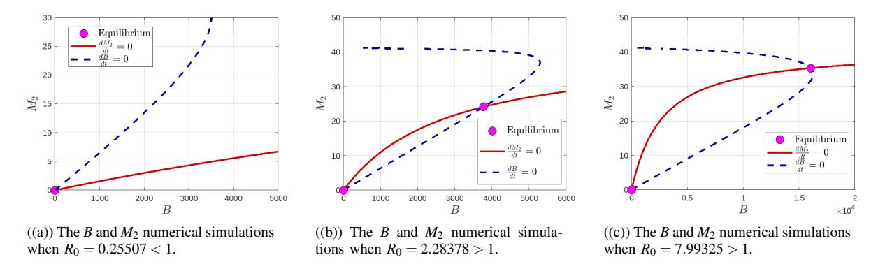
Figure 2: The graph of functions \(f_1\) (solid) and \(f_2\) (dash) defined in (21) and \(R_0 \le 1\) by using parameter values from Table 1.
| Parameter | range | column 3 | column 4 | column 5 | Units | Reference | |
|---|---|---|---|---|---|---|---|
| \(s_1\) | (3300-7000) | 5000 | 5000 | 5000 | 1/day | [36] | |
| \(d_1\) | (0.01-0.011) | 0.01 | 0.01 | 0.01 | 1/day | [36] | |
| \(d_2\) | (0.01-0.011) | 0.01 | 0.01 | 0.01 | 1/day | [36] | |
| \(d_3\) | (0.01-0.011) | 0.01 | 0.01 | 0.01 | 1/day | [36] | |
| β | \((10^{-8}-10^{-5})\) | \(3*10^{-8}\) | \(3*10^{-8}\) | \(3*10^{-8}\) | 1/(cell · day) | [13] | |
| \(\alpha_1\) | - | \(6*10^{-3}\) | \(6*10^{-4}\) | \(6*10^{-4}\) | 1/(cell · day) | - | |
| \(\alpha_2\) | \((2*10^{-5}-3*10^{-5})\) | \(2*10^{-5}\) | \(2*10^{-6}\) | \(2*10^{-6}\) | 1/(cell · day) | [26] | |
| \(\mu_2\) | (0.05-0.5) | 0.11 | 0.11 | 0.11 | 1/day | [13] | |
| r | (0-0.26) | 0.005 | 0.005 | 0.005 | 1/day | [36] | |
| \(d_5\) | - | 0 | 0 | 0 | 1/day | ||
| \(k_1\) | \((1.25 * 10^{-9} - 1.25 * 10^{-7})\) | \(8*10^{-8}\) | \(8*10^{-8}\) | \(3*10^{-8}\) | 1/(cell · day) | [13] | |
| \(k_3\) | \(1.25 * 10^{-7}\) | \(1.25 * 10^{-7}\) | \(1.25 * 10^{-7}\) | \(1.25 * 10^{-7}\) | 1/(cell · day) | [36] | |
| N | (50-100) | 50 | 50 | 50 | constant | [36] | |
| S4 | 1000 | 1000 | 1000 | 1000 | 1/day | [36] | |
| γ | - | 0.008 | 0.008 | 0.008 | 1/(cell · day) | [43] | |
| \(d_4\) | - | 0.33 | 0.33 | 0.33 | 1/day | [36] | |
| p | - | 0.5 | 0.5 | 0.5 | constant | ||
Table 1: Information is inferred from published works (references).
Figure (4) shows that in this case, a numerical simulation of the model is shown when immune cell capacity decreases with decreasing parameter values \(\alpha_1\) and \(\alpha_2\) to \(6*10^{-4}\) and \(2*10^{-6}\), respectively. The resulting value of \(R_0\) is 2.28378. Infected macrophages (M2) continue to increase with increasing extracellular bacterial particles (B) to a maximum value, then decrease to an endemic equilibrium point. Healthy macrophages, activated macrophages, and naive T cells also increase to a maximum value, then decrease to an endemic equilibrium point. This indicates that the body's immune system cannot completely eliminate infected macrophages (M2) and extracellular bacterial particles (B). Immune cells (T cells) that can differentiate into cytotoxic T cells or helper T cells are unable to control and eliminate Mtb bacterial infection, allowing extracellular bacterial particles (B cells) to continuously infect healthy macrophages (M1 cells). Consistent with findings published by [14], a peak in the bacterial (B cell) and infected macrophage (M2) populations was observed early in the infection. These results indicate that M0 cells are highly susceptible to competition between Mtb bacteria, macrophages, and immune cells. These findings may help explain the need for the immune system to deploy stronger defense mechanisms to prevent Mtb infection, as macrophage
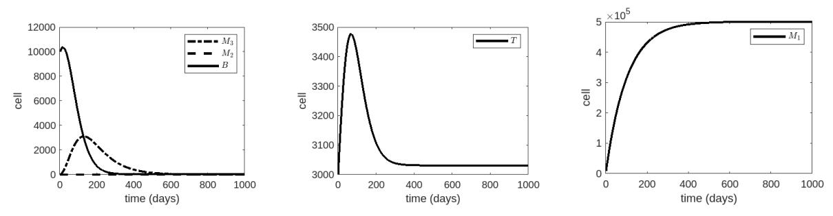
Figure 3: System numerical simulations (6). The graphs, which use the parameter values listed in Table 1, column 3, display the time course of bacteria, T cells, and uninfected, infected, and activated macrophages. In this instance, Mtb is eliminated, and \(R_0 = 0.25507\).
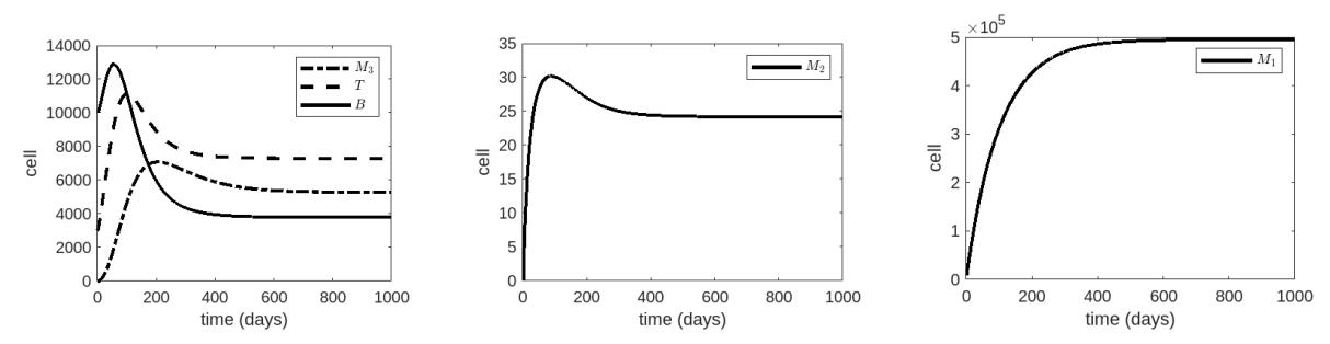
Figure 4: System numerical simulations (6). The graphs, which use the parameter values listed in Table 1, column 4, display the time course of bacteria, T cells, and uninfected, infected, and activated macrophages. In this instance, the progression of Mtb is regulated and \(R_0 = 2.28378\).
responses alone are insufficient to halt the initial bacterial invasion. The activity of immune cells (T cells) and macrophages allows for the regulation of bacterial growth and the immunological response that occurs concurrently with granuloma formation [47]. These theoretical findings suggest a trend toward an endemic equilibrium, meaning that bacterial, macrophage, and immune cell populations coexist. The condition \(R_0 > 1\) has been confirmed to be satisfied, resulting in a locally asymptotically stable endemic equilibrium point. Table 1 column 4 are used to illustrate the dynamic of the population of B and B in Figures (4). As demonstrated by the phase portrait and temporal evolution of B with ten initial conditions in Figure (6(b)) and Figure (7(b)). It is confirmed that conditions B 1 are satisfied, leading to a unique endemic equilibrium B 1 that is locally asymptotically stable, as indicated by Theorem (3.5).
If a small number of bacteria are injected, the model will proceed to either primary TB or clearance, contingent upon various parameter values. Infections leading to active TB are referred to as primary TB [5]. With parameter values taken from Table 1, column 5, Figures (5) depict the behavior of bacteria and cell populations for \(k_1 = 3*10^{-8}\). We note that in this case \(R_0 = 7.99325\), the population of T cells cannot activate rapidly enough to stop the infection. Although T cell counts begin to increase quickly, they eventually fail to control infection. The number of infected macrophages drops precipitously as a result of their burst. As a result, a significant amount of intracellular bacteria is released, leading to the growth of the out-of-control population of bacteria. Such a high bacterial load can cause necrosis, cavity formation, and spread [36]. The results presented in [50],[37], [46] are in line with this scenario. Furthermore, a particularly virulent strain of mycobacteria or an immunosuppressed host may be responsible for the rapid progression to primary TB. This is probably caused by immune system failure [37]. \(E_1\) is locally asymptotically stable, according to Theorem 3.5. This corresponds to the figures (6(c)) and (7(c)), which depict the phase portrait and the temporal evolution of the bacteria under varying initial conditions (denoted by circle) and final points denoted
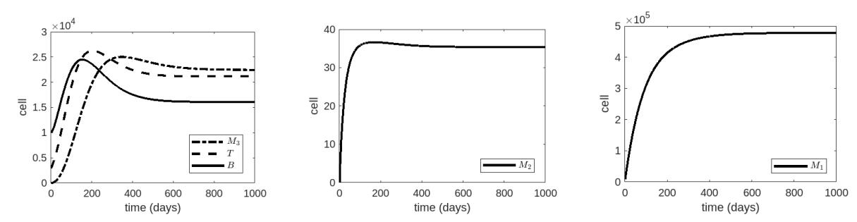
Figure 5: System numerical simulations (6). The time course of bacteria, T cells, and uninfected, infected, and activated macrophages are depicted in the graphs using parameter values from Table 1, column 5. In this case, Mtb is not controlled and R0 = 7.99325.
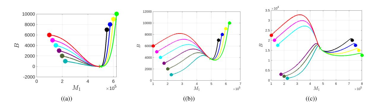
Figure 6: Portrait of phase fields for different initial conditions displays endemic and disease-free equilibrium points using the parameter values listed in Table 1.
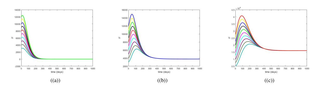
Figure 7: Using parameter values from Table 1, the numerical simulations of the temporal course for bacteria with ten initial conditions demonstrate the stability of the infection-free equilibrium E0 and the endemic equilibrium E1 comparing the three cases: (a) Mtb is eliminated, (b) Mtb progression is controlled, and (c) and Mtb is not controlled.
by x. Both the bacterial and immune T cell populations were seen to proliferate early in the infection, then decline until eventually approaching a steady state.
4.1. Sensitivity Analysis
Remember that when all other cell populations are fully susceptible, \(R_0\) represents the expected total number of new infectious particles produced by a single infectious particle (bacteria) during its average life span [49], [20]. The basic reproductive ratio, \(R_0\), is used to provide qualitative analysis of the models.
\[R_{0} = \frac{\beta s_{1} N \mu_{2}}{d_{1} \sigma \sigma_{1}}\] \[= \frac{\beta s_{1} N \mu_{2}}{d_{1} (d_{2} + \mu_{2} + \frac{s_{4} (\alpha_{1} p + \alpha_{2} (1 - p))}{d_{4}})(-r + d_{5} + \frac{k_{1} s_{1}}{d_{1}})}\] \[= \frac{\beta s_{1} N \mu_{2}}{(d_{2} + \mu_{2} + \frac{s_{4} (\alpha_{1} p + \alpha_{2} (1 - p))}{d_{4}})(-r d_{1} + d_{5} d_{1} + k_{1} s_{1})},\] (42)
where \(d_2\) and \(d_5\) represent the natural death rates of infected bacteria and macrophages, respectively, and r is the average number of bacteria produced as a result of self-replication; The rate of bacterial death by uninfected macrophages is \(k_1\), \(\beta\) is the infection rate; The removal rates of infected macrophages by pT and (1-p)T, respectively, are denoted by \(\alpha_1\) and \(\alpha_1\); p is the proportion of differentiated naive T cells; \(\mu_2\) is the maximal bursting rate of infected macrophages. The best way to reduce the number of mtb bacteria is to assess the sensitivity of various factors responsible for their transmission and prevalence. This study used a local sensitivity analysis. The index definition sensitivity can be seen in [9]. It should be noted that if the sensitivity index value is greater, then this parameter is the most influential. Positive and negative signs indicate the relationship between the parameter and the variable. Given that \(R_0\) (42) has an explicit formula, we can calculate the sensitivity of \(R_0\) to each of the parameters listed in Table 1, column 5. For example, the sensitivity indices of \(R_0\) for \(\beta\) are independent of any parameter value.
\[\Upsilon_{\beta}^{R_0} = \frac{\partial R_1}{\partial \beta} \times \frac{\beta}{R_1} = 1.\]
A few partially significant indices with a clear structure are as follows:
\[\Upsilon_{k_{1}}^{R_{0}} = \frac{\partial R_{0}}{\partial k_{1}} \times \frac{k_{1}}{R_{0}} = -\frac{k_{1}s_{1}}{\left(-r + d_{5} + \frac{k_{1}s_{1}}{d_{1}}\right)d_{1}} = -1.5,\] \[\Upsilon_{\alpha_{1}}^{R_{0}} = \frac{\partial R_{0}}{\partial \alpha_{1}} \times \frac{\alpha_{1}}{R_{0}} = -\frac{\alpha_{1}ps_{4}}{\left(d_{2} + \mu_{2} + \frac{s_{4}(\alpha_{1}p + \alpha_{2}(1 - p))}{d_{4}}\right)d_{4}} = -0.88079.\]
Table 2 presents a summary of our findings regarding the sensitivity of the basic reproductive ratio. The positive symbol indicates that the basic reproductive ratio will increase as the parameters increase. For each variation 1% in the parameter, the figure indicates how the basic reproductive ratio will change. For example, increasing 1% of the elimination rate \(\alpha_1\) will decrease \(R_0 - 0.88079\%\) since \(\Upsilon^{R_0}_{\alpha_1} = -0.88079\). As can be seen, the most important parameters in the basic reproductive ratio are \(r, k_1, \beta, \mu_2\), and \(\alpha_1\).
These findings indicate that \(R_0\) is highly susceptible to the Mtb bacteria's production and release by macrophages. These results for \(R_0\) may contribute to understanding why the immune system requires more complex defensive mechanisms to contain Mtb-causing infections, such as the recruitment of different components of the immune system and the formation of granulomas, because an initial bacterial invasion cannot be controlled by the macrophage response alone.
In Figure 8(a), it can be seen that when parameter r is in the value range \(0 < r < r^*\), with
\[r^* = \frac{-N\beta s_1\mu_2 + (k_1s_1 + d_1d_5)\sigma}{\sigma d_1} = 0.03107\] there is only one equilibrium point, namely the disease-free
Table 2: \(R_0\) (42) sensitivity indices to Mtb Infection model parameter values from Table 1
| β | r | \(\mu_2\) | \(\alpha_1\) | \(\alpha_2\) | \(k_1\) | \(d_2\) | \(d_5\) | |
|---|---|---|---|---|---|---|---|---|
| \(\Upsilon^{R_0}\) | 1 | 0.5 | 0.89342 | -0.88079 | -0.00293 | -1.5 | -0.00968 | 0 |
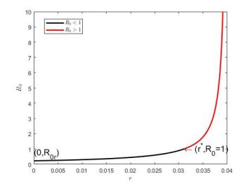
- ((a)) Plot of the first quadrant's existence and stability (r and \(R_0\)).
- ((b)) Plot of the first quadrant's existence and stability (\(\alpha_1\) and \(R_0\)).
- ((c)) Plot of the first quadrant's existence and stability \((k_1 \text{ and } R_0)\).
Figure 8: The parameter values listed in Column 1 of Table 1.
equilibrium point indicated by the value \(R_0 < 1\). For the value 0 < r < 0.03107, the bacterial model of Mtb will always be stable in a disease-free state. Meanwhile, if parameter r, \(0.03107 < r < d_5 + \frac{k_1 s_1}{d_1} = 0.04\) causes \(R_0 > 1\) and the disease-free equilibrium point becomes unstable. This shows that the body's immune system cannot eliminate Mtb bacterial infections which result in the bacteria always being present in the lungs and continuing to infect uninfected macrophage cells.
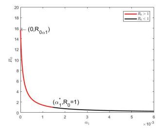
As seen in Figure 8(b), there is only one equilibrium point, which is the disease-free equilibrium point, indicated by the value \(R_0 < 1\), when parameter \(\alpha_1\) is in the value range \(\alpha_1 > \alpha_1^*\), with
\[\alpha_1^* = \frac{N\beta s_1 \mu_2 d_4 + \sigma_1 d_1 (-\alpha_2 (1 - p) s_4 - d_4 (d_2 + \mu_2))}{p\sigma_1 s_4 d_1} = 1.45651 * 10^{-3}.\] The Mtb bacterial model will always be stable in a disease-free state for the value \(\alpha_1 > 1.45651 * 10^{-3}\). Meanwhile, if \(0 < \alpha_1 < 1.45651 * 10^{-3}\) causes \(R_0 > 1\) and the disease-free equilibrium point to become unstable. This shows that a reduced immune system causes bacteria to remain in the lungs and can infect uninfected macrophage cells.
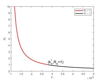
As can be observed in Figure 8(c), when parameter \(k_1\) is in the value range \(k_U > k_1^*\), there is only one equilibrium point, which is the disease-free equilibrium point, denoted by the value \(R_0 < 1\), with \(k_1^* = \frac{N\beta s_1\mu_2 + (r - d_5)\sigma d_1}{2} = 2.785480062*10^{-8}\). If \(k_1 > 2.785480062*10^{-8}\), then the Mtb bacterial model will
remain stable in a disease-free state at all times. Meanwhile, if \(R_0 > 1\) and the disease-free equilibrium point becomes unstable due to parameter \(10^{-8} < k_1 < 2.785480062*10^{-8}\). This demonstrates how the decreased ability of uninfected macrophages to fight off bacteria leads to the persistence of bacteria in the lungs and their ability to infect uninfected macrophage cells.
5. CONCLUSION
In this study, we investigated the effects of patient immune control and proliferation of the TB bacterial population on the development of tuberculosis disease. For this reason, we developed a system of non-linear ordinary differential equations that concisely characterize Mtb's interactions with macrophages and T cells. Numerous studies have described the intricate processes of cell differentiation and activation that comprise the immune response to tuberculosis infection [50], [46]. However, modeling all of these processes is challenging, so we only take into account the most significant ones.
The model developed in this work became necessary to supplement the earlier research provided in [27], [22], [28] [24], [29], [36], [25], [26]. Here, we assume that there are two types of bacterial growth: the first is internal bacterial growth, as described in earlier research, and the second is external bacterial growth caused by self-replication and external bacteria from infected macrophage rupture owing to capacity limitations. Both presumptions are true [44], [31].
Naturally, as the assumptions get more complicated, so does the complexity of the results. A qualitative analysis of this model indicates various scenarios in which, subject to specific conditions, there is always an infection-free state. The existence of two different kinds of bi-stability region for a given parameter value is an intriguing fact. The first is the balance that exists in coexisting bacteria and is free of disease. However, a sensitive examination of the model parameters reveals why macrophages are insufficient to stop Mtb from invading the body in the first place and why the immune system must carry out more intricate defense mechanisms, such as forming granulomas and recruiting other components of the immune system, to contain the infection. In conclusion, in this study, we show that by including the self-replication of bacteria, the scenarios observed in the development of pulmonary tuberculosis can be obtained more diverse.
ACKNOWLEDGEMENT
Parts of this article were funded by a research grant.
AUTHORS' CONTRIBUTION
All the authors of this article were the main contributors to the writing of this article.