

1. INTRODUCTION
Mycobacterium tuberculosis is the cause of tuberculosis (TB), a disease that can affect every organ in the body but is most common in the lungs [25], [8], [21], [7]. TB disease tends to attack individuals who have weakened immune systems, such as people with HIV/AIDS [26]. Significant cases of tuberculosis were reported in Indonesia, with West Java ranking highest among the provinces with the largest populations, particularly in East Java, Central Java, and West Java [39]. Several studies have highlighted the importance of TB mapping in addressing the spread of the disease [4], [1]. The studies make the case that by comprehending the TB mapping pattern, suitable countermeasures might be designed to stop the disease's spread.
Factors that differ from place to place affect the transmission of tuberculosis [22]. With such diverse factors in each region, spatial analysis is needed to geographically map the distribution of TB disease [31], [32]. According to Chen et al., 2023 [10], the Geographically Weighted Regression (GWR) approach was used to determine the impact of Kashgar's population, gross product per capita, and the amount of healthcare facilities
*Corresponding author
Received July 26th, 2024, Revised March 19th, 2025, Accepted for publication June 15th, 2025. Copyright ©2025 Published by Indonesian Biomathematical Society, e-ISSN: 2549-2896, DOI:10.5614/cbms.2025.8.1.6
per capita on the prevalence of tuberculosis. Using spatial analysis through these methods can result in each region being affected by different variables [17], [34]. In this method, a kernel function will be applied. The weighting function at each position makes up the members of the diagonal matrix that represents the kernel function. There are various approaches for this kernel function, such as Gaussian, Exponential, Triangular, Uniform, Quadratic, and Bi-Square [43].
However, the incidence of TB cases in each region may vary over the years. The number of TB cases can increase or decrease depending on the region. Due to the relationship between one region and another over a period of several years, spatial analysis alone is no longer sufficient [14]. Therefore, a spatio-temporal analysis approach is needed to replace the GWR method, which cannot be applied in this context [9]. In the research [48], the development method of GWR, Geographically and Temporally Weighted Regression (GTWR), was used. The research indicates that tuberculosis (TB) in China is influenced by multiple factors, including medical and health care, transportation, economic conditions, and educational standards. By using this model, we can find out that each year, the region is affected by different variables. In GTWR approach, the same bandwidth is used for each observation [24]. In local regression analysis, bandwidth refers to the separation or quantity of neighbors [12]. The higher the bandwidth value, the more locations are used. Another approach, Multiscale Geographically and Temporally Weighted Regression (MGTWR), uses different bandwidths for each observation and it has been proven to be more effective than the GTWR method.
MGTWR extends the GTWR approach by using a flexible bandwidth on the variables for each observation [45]. It allows us to explore spatio-temporal variation more effectively than GTWR. With reference to the research [44] that examines the investigation of the factors influencing Shenzhen house prices, MGTWR's results were more useful than GTWR's since they showed the outcomes for each location impacted by different variables between 2010 and 2017. However, this study did not explain the method of using any kernel function. While previous studies have applied various spatial models for TB mapping, none have utilized the MGTWR approach. This study provides a novel contribution by integrating spatial and temporal variations in TB incidence through MGTWR and comparing its performance with the GTWR model. This research insights provide a deeper understanding of region-specific and time-sensitive factors influencing TB cases, which previous models have overlooked. These findings could enhance targeted public health interventions and optimize resource allocation for effective TB control.
In regression, it is known that there is multicollinearity in the data. Strong relationships or correlations between predictor variables are known as multicollinearity, and they have an impact on how the results are interpreted [37]. To overcome this multicollinearity problem, this research will use the Least Absolute Shrinkage and Selection Operator (LASSO) variable selection method [19]. Nevertheless, this method still has the disadvantage of not balancing the influence of different variables. There is a development of LASSO, namely Adaptive LASSO [49], which is proven to be more effective in overcoming multicollinearity problems in the data. Adaptive LASSO provides adaptive penalty weights so as to produce variables that actually have a real effect on TB cases. Hence, this research will modify the usage of variable selection prior to being incorporated into the GTWR and MGTWR models by employing kernel variations (Gaussian, Exponential, Uniform, and Bi-Square) that differ from those used in earlier research. Since they result in singular matrices, quadratic and triangular kernels are not employed. This improvisation will yield the optimal model for TB mapping, which will identify the variables that actually have an impact in each region.
The next part of this paper will describe the dataset used for research, variable selection, MGTWR modeling in Section 2, present variable selection results, assumption tests, model comparison, and mapping in Section 3, and offer conclusions in Section 4.
2. METHODS
2.1. Dataset
The study utilizes the number of TB cases in West Java Province as the response variable, categorized by districts or cities, sourced from BPJS (Badan Penyelenggara Jaminan Sosial) data that can be accessed from the public domain (https://data.bpjs-kesehatan.go.id/bpjs-portal/). This response variable represents the total number of confirmed TB cases recorded in the BPJS dataset from 2019 to 2022, categorized by districts or cities in West Java Province. The predictors were obtained from the West Java Provincial Government's official open data portals, such as Open Data Jabar (https://opendata.jabarprov.go.id/id) and the West Java Central Bureau of Statistics (https://jabar.bps.go.id/). Three global climate variables from the Copernicus
Climate Data Store are also used as predictors (https://climate.copernicus.eu/). The dimensions and variables utilized in this research are displayed in Table 1. Z-score normalization is applied to all data, rescaling it to a mean of 0 and a standard deviation of 1 [18].
In statistical regression, data analysis generally utilizes the entire dataset for training and evaluation without separation, especially when the data is limited. This contrasts with machine learning, which partitions the data to avoid overfitting and ensure model generalization to new data. Moreover, statistical regression must satisfy fundamental assumptions such as normality, which ensures that residuals are normally distributed; homoscedasticity, which ensures constant residual variance; and the absence of multicollinearity among independent variables. If these assumptions are not met, regression results may become biased or unreliable. Additionally, statistical regression emphasizes understanding the relationships between variables, which is why this approach utilizes the entire dataset in the analysis process.
In this study, model evaluation was conducted using R2 to measure the strength of variable relationships and the Akaike Information Criterion (AIC) to assess the balance between model complexity and parameter estimation quality.
Table 1: Dimensions and variables that will be used in the research.
| Dimensions | Descriptions | Variables |
|---|---|---|
| Total Daily Average Air Temperature | xair | |
| Global Climate | Total Daily Precipitation Rainfall | xrain |
| Total Daily Average Relative Humidity | xhum | |
| Number of Hospitals | xhos | |
| Number of Nursing Workers | xnurse | |
| Percentage of Low Birth Weight Babies | xbabies | |
| Number of Laboratory Technologists in Hospitals | xlab | |
| Number of Specialist Doctors | xdoc | |
| Health | Proportion of Households with Adequate Sanitation Facilities | xsanit |
| Health Index | xhealth | |
| Number of Active Integrated Health Service Posts | xpos | |
| Number of Villages that Stop Open Defecation | xdef | |
| Number of Villages that Have Pharmacy Facilities | xphar | |
| Proportion of households with access to safe drinking water | xwater | |
| Number of Males | xmales | |
| Number of Females | xfemale | |
| Count of Participants in Active Family Planning | xfamily | |
| Proportion of Households with Access to Affordable Housing | xhome | |
| Demographic | The Community Forest Area | xarea |
| Poverty Line | xpov | |
| Poverty Depth Index | xdepth | |
| Total Population Migrating In | xmigrating | |
| Life Expectancy | xlife | |
| Percentage of Poor People | xpoor | |
| Population Density | xpop | |
| Employees in Micro and Small Businesses | xmicro | |
| Proportion Engaged in the Workforce | xf orce | |
| Social | Rate of Open Unemployment | xunemployment |
| Human Development Index | xhuman | |
| Education Index | xedu | |
| Gender Development Index | xgender | |
| Gender Empowerment Index | xempowerment | |
| Expenditure Index | xexpenditure | |
| Proportion of Households that Practice Healthy and Clean Habits | xclean | |
| Government Policy | Proportion of Households Utilizing Safely Managed Sanitation Service | xsaniservice |
| Proportion of Households Utilizing Safe and Managed Drinking Water Services | xdrinkservice |
2.2. Variable selection
Regression analysis is a basic statistical technique used to model the relationship between a dependent variable and one or more independent variables. One of the most commonly used regression methods is multiple linear regression, where the relationship is assumed to be linear. In this approach, the Ordinary Least Squares (OLS) method is usually used to estimate the regression coefficients by minimizing the residual sum of squares. However, OLS has major limitations in that it does not perform variable selection and can lead to overfitting, especially when dealing with high-dimensional data. To overcome this issue, statisticians developed the Least Absolute Shrinkage and Selection Operator (LASSO) method. LASSO improves OLS by incorporating a penalty term L1 that minimizes the sum of squared residuals while constraining the absolute values of the regression coefficients [5]. This penalty forces some coefficients to shrink to zero, effectively performing variable selection and improving model interpretability. Because of its ability to handle highdimensional data and reduce overfitting, LASSO has become a widely used technique in statistical modeling and machine learning. The parameter β in LASSO is estimated as follows [16]:
\[\hat{\beta} = \operatorname{argmin} \left\{ \sum_{i=1}^{n} (y_i - \beta_0 - \sum_{j=1}^{p} \beta_j x_{ij})^2 \right\}.\] (1)
The response variable for the i-th observation is denoted by yi in the Equation 1; the predictor variables are denoted by x; the value of the j-th predictor variables for the i-th observation is represented by xij ; and the regression coefficient for the j-th predictor variables is represented by βj . Despite its advantages, LASSO applies the same shrinkage penalty to all coefficients, which biases the estimates of significant variables. The researchers developed Adaptive LASSO to address this issue by assigning different penalty weights to each coefficient. This improvement allows for more precise estimation while maintaining the benefits of regularization and variable selection.
The Adaptive LASSO method assigns weighted penalties to each regression coefficient, allowing researchers to obtain a more stable model with fewer exactly zero coefficients compared to the standard LASSO method [28]. Unlike LASSO, which applies uniform shrinkage, Adaptive LASSO reduces bias by assigning different penalty weights to each coefficient. This approach helps retain significant predictors more effectively. This method follows a two-step procedure. First, researchers estimate a weight vector ωˆ based on the OLS estimates of βinit. The weight vector depends on the initial estimates and follows this formulation [13]:
\[\hat{\omega} = \frac{1}{|\hat{\beta}_{init}|^{\gamma}},\tag{2}\] where βˆ init represents the initial coefficient estimate, and γ is a positive constant, typically set to 0.5, 1, or 2. In the next step, researchers apply the penalty parameter λ to control the degree of regularization, influencing which variables remain in the model. The Adaptive LASSO estimation problem follows this formulation:
\[\hat{\beta} = \operatorname{argmin}_{\beta} \|y - \sum_{j=1}^{p} x_j \beta_j\|^2 + \lambda_n \sum_{j=1}^{p} \hat{\omega}_j |\beta_j|.\] (3)
Researchers frequently apply Adaptive LASSO in empirical studies because it balances variable selection and regularization. In practice, they determine λ and γ using cross-validation to optimize predictive performance. Many computational tools, such as the glmnet package in R and Python, offer efficient implementations for solving the Adaptive LASSO problem.
2.3. Multiscale Geographically and Temporally Weighted Regression
GTWR extends the GWR model by incorporating temporal variations to capture both spatial and temporal non-stationarity. The GTWR model is formulated as follows [15]:
\[y_i = \beta_0(u_i, v_i, t_i) + \sum_{k=1}^p \beta_k(u_i, v_i, t_i) x_{ik} + \varepsilon_i, \tag{4}\] where (ui , vi , ti) represents the space-time coordinate of the i-th sample; βk(ui , vi , ti) is the estimated coefficient of the k-th variable for that sample; and assuming a normal distribution, εi represents the ith residual value. Like GWR, GTWR uses the Weighted Least Squares (WLS) approximation method for calibration.
The kernel function determines the spatial and temporal weights assigned to each observation in a geographically weighted analysis. The kernel function \(\mathcal{K}(u)\) is a continuous function used to compute these weights. Some types of kernel functions are as follows [3], [42]:
1) Gaussian kernel:
\[w_{ij} = \exp\left(-\left(\frac{1}{2}\left(-\frac{|d_{ij}^{sT}|}{b}\right)^2\right)\right). \tag{5}\]
2) Exponential kernel:
\[w_{ij} = \exp\left(-\left(\frac{1}{2}\left(-\frac{|d_{ij}^{sT}|}{b}\right)\right)\right). \tag{6}\]
3) Uniform kernel:
\[w_{ij} = \begin{cases} \frac{1}{n_i^l}, & \text{j is neighbor of i in the 1-th order,} \\ 0, & \text{otherwide.} \end{cases}\] (7)
4) Bi-Square kernel:
\[\text{[rumus tidak dapat ditampilkan dengan baik — lihat PDF asli]}\](8)
where from the four kernel functions above, n is the number of observations, \(w_{ij}\) is the kernel weight of the i-th and j-th locations, \(d_{ij}^{sT}\) is the euclidean distance of the i-th location to the j-th location, Through the use of cross-validation (CV), which shows how close each location is to another, the bandwidth b is calculated.
A spatio-temporal distance function integrates the effects of spatial and temporal distances, as shown below [38]:
\[\begin{cases} (d_{ij}^s)^2 = (u_i - u_j)^2 + (v_i - v_j)^2, \\ (d_{ij}^T)^2 = (t_i - t_j)^2, \\ (d_{ij}^{sT})^2 = \phi^s[(u_i - u_j)^2 + (v_i - v_j)^2] + \phi^T[(t_i - t_j)^2]. \end{cases}\] (9)
where the weights \(\phi^s\) and \(\phi^T\) balance the impacts of space and time, which are measured in separate units. A development of the GTWR model led to the Multiscale Geographically and Temporally Weighted Regression (MGTWR), which enhances flexibility in capturing spatial and temporal variations. Unlike GTWR, MGTWR employs a flexible bandwidth approach, allowing each predictor to have distinct spatial and temporal bandwidths. This flexibility improves model accuracy by adapting to varying spatial and temporal scales across different variables. MGTWR applies an iterative back-fitting algorithm to estimate parameters, refining bandwidth selection for each variable. The general form of the MGTWR model is as follows [44]:
\[y_i = \beta_{bwt_0s_0} + \beta_{bwt_1s_1} \otimes x_1 + \dots + \beta_{bwt_ps_p} \otimes x_p + \varepsilon_i, \tag{10}\] where the symbol '\(\otimes\)' indicates the element-wise multiplication of two vectors, and the estimated coefficients of the p-th variables are represented by \(\beta_{bwt_ps_p}\) using certain spatial \(\beta_{bws_p}\) and temporal bandwidths \(\beta_{bwt_p}\). Using the GTWR model, the back-fitting algorithm initially sets up an additive term vector \(f_j\):
\[f_i = [f_{1i}, f_{2i}, ..., f_{ni}], \tag{11}\]
This algorithm modifies each unknown term separately based on the assumption that all other terms are known. At this stage, the residual term \(\hat{\varepsilon}\) can be obtained from:
\[\hat{\varepsilon} = \hat{y} - \sum_{j=1}^{m} \hat{f}_j. \tag{12}\]
Using the additive value of vector \(f_1\) to vector \(f_j\), the beta value is determined iteratively. This procedure seeks to acquire the best bandwidth for the new variable, and residual values are computed. This cycle is reiterated until the optimal bandwidth for all variables is determined.
3. RESULTS AND DISCUSSION
In the subsequent section, we will estimate the optimal selection parameter λ, predict significant variables and groups of variables, examine outliers and classical assumptions, identify the best model, and map the significance of each important variable or variable group. The models employed for this analysis are GTWR and MGTWR, utilizing LASSO and Adaptive LASSO variable selection techniques. Additionally, we will utilize four different kernels (Gaussian, Exponential, Uniform, Bi-Square) for each model to determine the most effective mapping model for TB cases in West Java.
3.1. Selection of Important Variables
The Mean Squared Error (MSE) of the LASSO and Adaptive LASSO Cross-Validation (CV) processes is shown in Figure 1 and Figure 2. In the LASSO CV process, usually 5 or 10 folds are used in the process [27]. The lambda value with the lowest MSE value is used by the LASSO and Adaptive LASSO procedures [41]. In this research, the lambda values for LASSO and Adaptive LASSO respectively are 0.0010003 and 0.01.
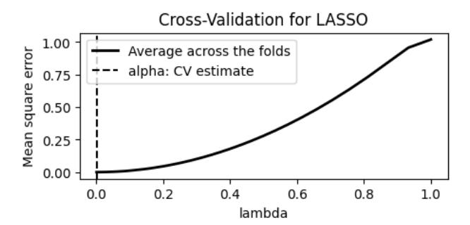
Figure 1: MSE plots of CV LASSO.
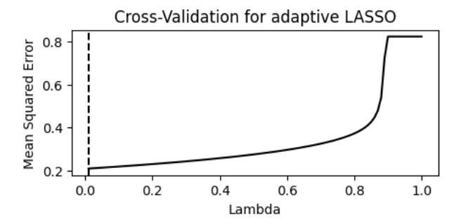
Figure 2: MSE plots of CV Adaptive LASSO.
Table 2 display the optimal LASSO and Adaptive LASSO models with significant variables determined by the smallest MSE using the best lambda. Subsequently, classical assumptions will be verified before model implementation.
Methods Variables Selection LASSO xrain, xhum, xphar, xpop, xsanit, xpoor, xgender, xwater, xpos, xnurse, xbabies, xclean, xdef, xlab, xgend, xexpen, xpov, xsaniservice, xdrinkservice, xforce, xmicro, xmales Adaptive LASSO xrain, xpop, xsanit, xpoor, xgender, xwater, xpos, xnurse, xbabies, xclean, xdef, xlab, xpov, xpovdep, xsaniservice, xhome, xmicro, xrate, xmales
Table 2: Important variables selection with LASSO and Adaptive LASSO.
3.2. Classical assumption test
In statistical modeling, essential classical assumption tests like the Kolmogorov-Smirnov normality test and the Breusch-Pagan heteroscedasticity test are performed [29], [35]. Both LASSO and Adaptive LASSO models in Table 3 exhibit normal distributions with p-values above 0.05, confirming the normal distribution hypothesis. Constant errors are present in both models, with p-values exceeding 0.05, indicating the absence of multicollinearity. The positive Moran's I test result for the LASSO model indicates clustered data features; however, the negative Moran's I test value for the Adaptive LASSO model indicates dispersed data characteristicss [40]. The Durbin-Watson value, which is seen to be between 0 and 2, supports the lack of autocorrelation assumptions in both models [2]. Figure 3 displays varying maximum values in boxplots, revealing temporal heterogeneity. The use of LASSO and Adaptive LASSO variable selection effectively addresses multicollinearity concerns in both datasets.
Table 3: Statistical test results for LASSO and Adaptive LASSO.
| Test | LASSO | Adaptive LASSO |
|---|---|---|
| Kolmogorov-Smirnov Normality Test | 0.7969 | 0.5103 |
| Breusch-Pagan Heteroscedasticity Test | 0.1932 | 0.3123 |
| Moran's I Test | 0.0188 | -0.008 |
| Durbin-Watson Test | 1.7101 | 1.9672 |
| Temporal Heterogeneity Test | Boxplot in Figure 3 | |
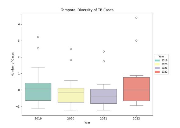
Figure 3: Boxplot of temporal diversity TB cases in 2019-2022.
3.3. Model comparison
Table 4 presents the accuracy of estimates for each model. The accuracy was assessed based on two criteria: the model with the highest R2 value and the lowest AIC value. A higher R2 indicates a better fit, while a lower AIC value suggests a more accurate model [33]. The best-performing model in this study is the MGTWR model utilizing LASSO on a Bi-Square kernel function. With a R2 of 0.91254 or about 91.25%, this model is able to account for 91.25% of the variability of TB values; the remaining 8.75% is explained by factors that are not part of the model. Furthermore, this model has the smallest AIC value among the other models, at 139.868. It is important to note that a smaller AIC value indicates a more accurate model.
| Model | GTWR | MGTWR | ||||||
|---|---|---|---|---|---|---|---|---|
| LASSO | adaptive LASSO | LASSO | adaptive LASSO | |||||
| 2 R | AIC | 2 R | AIC | 2 R | AIC | 2 R | AIC | |
| Gaussian | 0.90342 | 146.7689 | 0.89771 | 149.9971 | 0.88518 | 151.3207 | 0.87279 | 152.4452 |
| Uniform | 0.83924 | 156.0763 | 0.86087 | 155.9987 | 0.83924 | 156.0763 | 0.86087 | 155.9987 |
| Bi-Square | 0.90389 | 146.8986 | 0.89838 | 149.9372 | 0.91254 | 139.868 | 0.90486 | 140.3877 |
| Exponential | 0.89839 | 149.1443 | 0.83953 | 156.0705 | 0.89056 | 150.885 | 0.87768 | 152.2908 |
Table 4: Accuration comparison of GTWR and MGTWR models.
3.4. Best Model Mapping Results
After comparing the models, it is determined that the best model is the MGTWR with LASSO on the Bi-Square kernel function. Subsequently, a partial test is conducted to identify significant variables. A two-tailed t-test is applied with the following hypotheses:
H0 : βk = 0, k = 1, 2, ..., p (variable k is not significant)
H1 : βk ̸= 0, k = 1, 2, ..., p (variable k is significant)
If tvalues > ttable (positive) or tvalues < ttable (negative), the null hypothesis is rejected, indicating that the corresponding variable significantly influences tuberculosis cases. Out of the 22 LASSO selected variables in the best model, 11 variables significantly influence the number of TB cases, as shown in Table 5. Table 5 also displays the optimal bandwidth for each variable, where a larger bandwidth indicates that more locations are considered in the mapping process [47]. Furthermore, a set of significant variables affecting tuberculosis cases is identified. This mapping is further divided into two-year intervals based on the similarity of spatial regions and significant variables, namely 2019-2020 and 2021-2022, as shown in Table 6. Moving forward, the significance of each variable in different areas from 2019 to 2022 is visualized through mapping.
| Table 5: Significant coefficient and optimal bandwidth of each variable. | |||||
|---|---|---|---|---|---|
| Variables | Bandwidth | MGTWR Significant Coefficients | ||
|---|---|---|---|---|
| Min | Mean | Max | ||
| Xrain | 13 | 0.05 | 0.08 | 0.12 |
| Xhum | 117.5 | 0.19 | 0.27 | 0.34 |
| Xpop | 15.7 | 0.07 | 0.14 | 0.20 |
| Xgender | 21.7 | -0.42 | -0.27 | -0.11 |
| Xbabies | 117.3 | 0.42 | 0.73 | 1.04 |
| Xclean | 14.4 | -0.26 | -0.24 | -0.21 |
| Xpov | 15.1 | 0.40 | 0.47 | 0.53 |
| Xsaniservice | 117.5 | -0.29 | -0.25 | -0.21 |
| Xdrinkservice | 117.5 | -0.30 | -0.21 | -0.12 |
| Xf orce | 14 | 0.12 | 0.16 | 0.21 |
| Xmales | 11.5 | 0.23 | 0.46 | 0.69 |
| Year | Group | Regency/City | Variables |
|---|---|---|---|
| 2019-2020 | 1 | West Bandung, Bandung, Bekasi, Bogor, Ciamis, Cianjur, Cirebon, Garut, Indramayu, Karawang, Bandung City, Banjar City, Bekasi City, Bogor City | xrain, xpop, xbabies, xclean, xdrinkservice, xmales |
| 2 | Cimahi City, Cirebon City, Depok City, Suk abumi City, Tasikmalaya City, Kuningan, Ma jalengka, Pangandaran, Purwakarta, Subang, Suk abumi, Sumedang, Tasikmalaya | xhum, xpop, xgender, xclean, xpov, xsaniservice, xmales | |
| 2021-2022 | 1 | West Bandung, Bandung, Bekasi, Bogor, Ciamis, Cianjur, Cirebon, Garut, Indramayu, Karawang, Bandung City, Banjar City, Bekasi City | xrain, xpop, xbabies, xclean, xdrinkservice, xf orce, xmales |
| 2 | Bogor City, Cimahi City, Cirebon City, Depok City, Sukabumi City, Tasikmalaya City, Kuningan, Majalengka, Pangandaran, Purwakarta, Subang, Sukabumi, Sumedang, Tasikmalaya | xhum, xpop, xgender, xclean, xpov, xsaniservice, xmales |
Table 6: Significant variables groups of each region from 2019-2022.
The optimum regression form for mapping tuberculosis in West Java may be determined from Table 6. The regression equation will be shown for the Bogor region in 2019–2022, which is the region with the greatest instances from 2019–2022.
\[y_{Bogor2019} = 0.10597 + 0.0924X_{rain} + 0.0899x_{pop} + 1.036x_{babies} - 0.2634x_{clean} - 0.3031x_{drinkservice} + 0.6883x_{males} + \varepsilon_i,\] (13)
\[y_{Bogor2020} = 0.10597 + 0.0979X_{rain} + 0.0846x_{pop} + 1.038x_{babies} - 0.2565x_{clean} - 0.3031x_{drinkservice} + 0.6883x_{males} + \varepsilon_i,\] (14)
\[y_{Bogor2021} = 0.10595 + 0.1040X_{rain} + 0.0806x_{pop} + 1.039x_{babies} - 0.2503x_{clean} - 0.3031x_{drinkservice} - 0.2080x_{force} + 0.6873x_{males} + \varepsilon_i,\] (15)
\[y_{Bogor2022} = 0.10595 + 0.1107X_{rain} + 0.0750x_{pop} + 1.041x_{babies} - 0.2432x_{clean} - 0.3031x_{drinkservice} - 0.2162x_{force} + 0.6873x_{males} + \varepsilon_i.\] (16)
As seen in regression Equations 13, 14, 15, and 16, each year the Bogor region area has a different regression coefficient obtained from the best model. For example, the interpretation of the regression Equation 13 of Bogor region in 2019 is influenced by the variables of total daily precipitation rainfall, population density, the percentage of infants born with low body weight, the proportion of households that practice healthy and clean habits, the proportion of households utilizing safe and managed drinking water services, and the number of males. The intercept, or β0 value, is 0.10597, which means that with normalized data, approximately 0.10596 TB cases occur when all predictor variables are 0. The regression coefficient for the total daily precipitation rainfall variable, which is positive at 0.0924, shows that there is a positive association between the number of TB cases and the total daily precipitation rainfall using normalized data. The higher total daily precipitation rainfall in Bogor region, the more TB cases are found at 0.0924. In contrast to the variable of the proportion of households that practice healthy and clean habits, which has a coefficient value of -0.2634, the result of data normalization has a negative relationship to the number of TB cases. The greater the proportion of households that practice healthy and clean habits, the lower the value of the number of TB cases, worth -0.2634. The interpretation of positive and negative relationships also applies similarly to other regression variable values.
It can be seen that daily rainfall precipitation is positively associated with TB case numbers. Based on research [36], rainfall is also positively linked to TB case numbers. This is because rainfall creates a humid environment, which provides a favorable condition for the growth and spread of TB bacteria. Conversely, factors like the proportion of households that practice healthy and clean habits and the proportion of households utilizing safely managed drinking water services exhibit a negative correlation with TB case numbers.
There are seven variables that exhibit a positive correlation with the number of TB cases, namely total daily precipitation rainfall, total daily average relative humidity, population density, percentage of infants
born with low body weight, poverty line, the proportion engaged in the workforce, and number of males. Among the climate-related variables, both rainfall and humidity show a positive relationship, as humidity contributes to reduced exposure to sunlight causing the environment to become dark and humid [46]. In terms of gender, only males demonstrate a positive relationship with the number of TB cases. This aligns with research findings indicating that men are more susceptible to TB compared to women [20].
The proportion engaged in the workforce variable displays a distinct pattern in its impact on TB case numbers. In the years 2019-2020, it shows no significant influence on TB cases. However, in the years 2021- 2022, it becomes a significant variables. This change in behavior can be linked to the enactment of laws that limited community activities during the Covid-19 pandemic. With a decline in COVID-19 cases, the government allowed employees to return to their usual work schedules. As a result, the number of TB cases that have been detected has increased as a result of the limits being loosened.
The gender development index variable demonstrates a negative correlation with the number of TB cases [30]. This indicates that areas with greater gender equality tend to have fewer TB cases. Similarly, the proportion of households that practice healthy and clean habits, the proportion of households utilizing safely managed sanitation service, and the proportion of households utilizing safe and managed drinking water services also exhibit a negative correlation with the number of TB cases. These three variables fall under the government policy category, suggesting the effectiveness of policies implemented to address TB issues, particularly in promoting family and environmental hygiene. The data in Table 6 demonstrate that the incidence of tuberculosis cases varies by location due to several factors. From the grouping of time period/regency, it was discovered that the same factors consistently affected several regions from 2019 to 2022. These variables include total daily average relative humidity, population density, the gender development index, the proportion of households that practice healthy and clean habits, the proportion of households utilizing safely managed sanitation service, poverty line, and the number of males. Based on the results, the government can more easily determine policy by looking at the significant variables that are consistent from year to year.
To show how distinct the variables impact each location a plot map for each time period is provided in Figure 4 and Figure 5. The visual representation highlights how certain variables consistently influence specific regions over time, offering insights that are difficult to extract from tables alone. The maps in Figures 4 and 5 depict the spatial distribution of significant variable groups in West Java over two different time periods, 2019–2020 and 2021–2022. These maps illustrate how tuberculosis risk factors have changed across regions and over time.
Figure 4 presents two groups of significant variables, each represented by a different color. The siennacolored areas indicate regions influenced by total daily rainfall precipitation, population density, the percentage of low birth weight babies, the proportion of households practicing healthy and clean habits, the proportion of households using safe and managed drinking water services, and the number of males. The dark greencolored areas show regions affected by total daily average relative humidity, population density, the gender development index, the proportion of households practicing healthy and clean habits, the poverty line, the proportion of households using safely managed sanitation services, and the number of males. Figure 5 introduces an additional significant variable that is the proportion engaged in the workforce (Xforce) in previous yellow significant variable group displayed in Figure 4. This changes is represented in orange color in Figure 5.
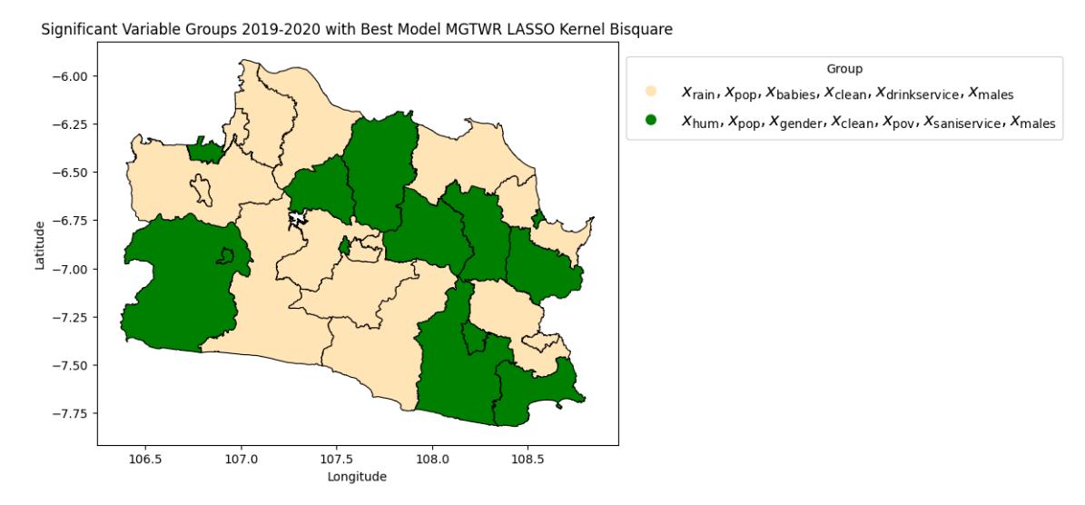
Figure 4: Variable group plot for each region in 2019-2020.
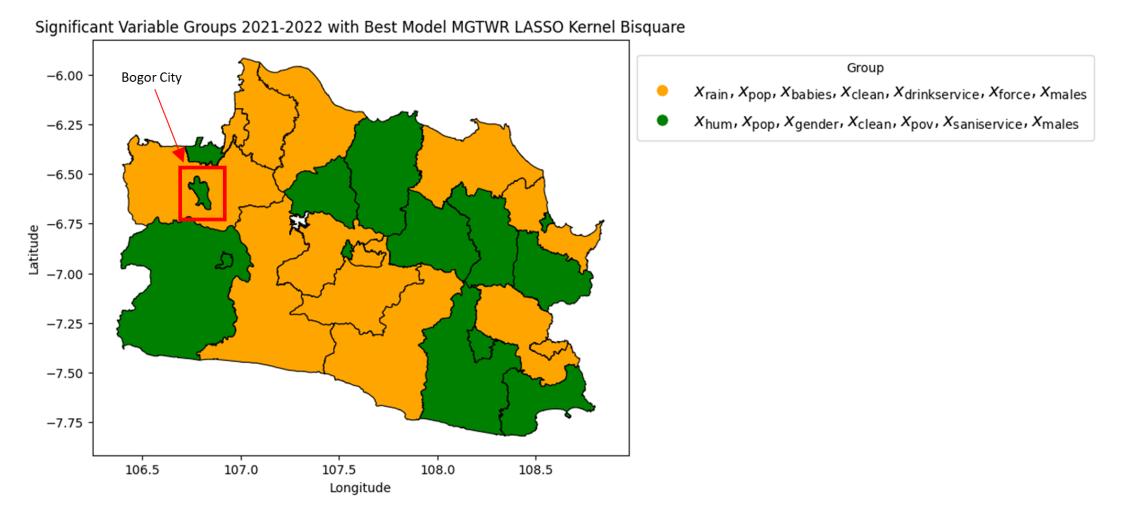
Figure 5: Variable group plot for each region in 2021-2022.
The appearance of Xforce in 2021–2022 highlights a shift in TB risk factors across several regions. This change indicates that workforce participation plays a more prominent role in tuberculosis dynamics during this period. Bogor City undergoes a significant transformation between the two periods. In 2019–2020, the significant factors influencing tuberculosis cases in Bogor City include total daily rainfall precipitation (Xrain), the proportion of households using safe and managed drinking water services (Xdrinkservice), and the percentage of low birth weight babies (Xbabies). However, in 2021–2022, these variables no longer play a significant role. This shift suggests that the factors contributing to tuberculosis cases in Bogor City have evolved, possibly due to environmental improvements, demographic changes, or shifts in disease transmission patterns. The emergence of Xforce in 2021–2022 likely stems from labor conditions during the COVID-19 pandemic. Industrial workers face a higher risk of severe TB and long-term complications due to exposure to chemicals, air pollution, UV radiation, and work-related stress [6]. A case study reveals that a delayed
diagnosis of cavitary TB in an industrial worker leads to post-TB lung disease (PTLD), which progressively worsens and results in premature death. These findings underscore the additional risks industrial workers face in TB progression, particularly in unhealthy working conditions without adequate pulmonary health monitoring. Figures 4 and 5 illustrate how dominant factors changed across different regions, reflecting the temporal dynamics of tuberculosis risk factors in West Java. Spatial visualization provides a clearer understanding of regional patterns compared to tabular data [11]. Therefore, these findings emphasize the need for policymakers to adjust intervention strategies in West Java based on the evolving significant variables in each time period.
4. CONCLUSION
The best representation model of factors affecting the number of TB cases based on \(R^2\) and AIC is MGTWR with LASSO on the Bi-Square kernel. This model has the highest \(R^2\) of 91.25% and the smallest AIC value of 139.868. Partially, the significant variables influencing TB cases in West Java from 2019 to 2022 is the total daily rainfall precipitation, total daily average relative humidity, population density, gender development index, percentage of low birth weight babies, proportion of households that practice healthy and clean habits, poverty line, the proportion of households utilizing safely managed sanitation service, the proportion of households utilizing safe and managed drinking water services, the proportion engaged in the workforce, and number of males.
The mapping results using the MGTWR method show a fairly good representation, where each region is clustered with the influence of different variables. These variables have various bandwidth values, reflecting the diversity of factors that affect each region specifically, which is in line with the findings of the research by Liu et.al, 2021 [23]. From 2019 to 2022, there is a consistent pattern for regions affected by the same variables in that period. This can be a reference for determining the right strategy to prevent the spread of TB in West Java.
Local governments could use the finding of this research as a guide when developing measures to stop the spread of tuberculosis cases in the West Java region. These findings can guide local government in managing TB by: (1) Strengthening the healthcare facilities, including improvement of access to healthcare workers and treatments. (2) Improving existing TB elimination program, notably in vulnerable population.
ACKNOWLEDGEMENT
This research was supported by Merdeka Belajar Kampus Merdeka (MBKM) program organized by Indonesia Defense University in collaboration with National Research and Innovation Agency (number: B/323/I/2024), and funded by the RIIM LPDP Grant and BRIN, contract number: B-3836/II.7.5/FR.06.00/11/2023.