

1. INTRODUCTION
Compartmental models are widely used to model the transmission of diseases [1]. Traditional models consider only a closed population within a patch. However, in a real-world scenario, it is significant to study the spread of the disease in multi-patch [2]. Human dispersal behaviors significantly influence the transmission of diseases because it is facilitated to interconnect the geographical or sociological distinct areas [3]. The optimal control theory is employed to identify the appropriate control strategies to reduce the size of the outbreak and decrease the number of infected individuals while minimizing the costs of implementing the control strategies [4]. The mathematical modeling and analysis of epidemic models with optimal control theory can be found in communicable diseases such as Rabies, Dengue, Malaria, Zika, Ebola, and COVID-19 [5], [6], [7], [8], [9], [12]. Drug distribution, quarantine, vaccination, self-protection policies (such as hand hygiene, face masks, sanitizers), and social distancing are examples of resources [1], [7], [13], [14].
The SARSCoV-2 virus caused the Coronavirus disease 2019 (COVID-19) [15]. It originated in December 2019 in Wuhan City, Hubei Province, China, and spread over 229 countries [15]. It is primarily transmitted when virus-containing droplets, aerosols, and airborne particles in the air and facilitates human-to-human transmission [15]. The disease globally spreads through human mobility. The World Health Organization (WHO) declared a pandemic in March 2020 [15]. In the initial stages of the novel disease, there are no specific or identified control or prevention strategies. According to WHO guidelines, countries have implemented several control strategies such as self-protection policies (hand hygiene, face masks, sanitizers, etc.), social distancing, self-quarantine, mandatory quarantine (private residences, hospitals, public institutions, etc.), and restrictions on human movements [16]. As of September 01, 2023, COVID-19 has resulted in 770,085,713 confirmed cases and 6,956,173 deaths worldwide [17].
The first confirmed case involving a Chinese tourist in Sri Lanka was reported on January 27, 2020, followed by the first local case on March 11, 2020 [18]. To control the situation, the government implemented a strict
*Corresponding author
Received May 1st, 2024, Revised November 29th, 2024, Accepted for publication December 20th, 2024. Copyright ©2025 Published by Indonesian Biomathematical Society, e-ISSN: 2549-2896, DOI:10.5614/cbms.2025.8.1.1
nationwide lockdown on March 20, 2020, to reduce the contact rate [19]. During this period, people faced several financial challenges due to economic failures locally and globally. On April 19, 2020, the government announced the relaxation of the strict lockdown by considering the spread of the disease as well as economic failure [19]. Inter-district travel was permitted only for essential service purposes. As of May 11, 2020, the country had partially reopened to offices and businesses under a set of health regulations such as selfprotection policies and social distancing [19]. But after much more time the government had to announce the strict nationwide lockdown and partial lockdown due to the spread of the disease [19]. Worldwide distribution of COVID-19 vaccinations began on December 08, 2020 [20]. Commencing on January 29, 2021, vaccination programs were initiated in Sri Lanka [21].
The initial epidemic model was proposed by Kermack and McKendrick in 1927, known as the SIR epidemic model [4]. The model was developed under the following assumptions: infected individuals are also infectious, the population is closed, no one from the outside enters the population and no one leaves the population and there are no births and deaths in the population and all recovered individuals have complete immunity and cannot be infected again.
To model the behavior of the transmission of diseases in multi-patch and multi-group or age-structure, Ross introduced a contact matrix in 1911 [22]. This matrix is used to collect re-scaled estimated levels of activity among interacting subgroups or age classes in heterogeneous mixing populations and captures the spatial spread of disease by using the Eulerian framework [23]. In 1955, S. Rushton and A. J. Mautner defined a deterministic model for more than one community, which was a more realistic model [24].
A patch residence-time matrix P is defined as the function of the human virtual dispersal behavior in the Lagrangian framework [25]. The risk of infection is a function of the residence time and local environmental risk. The transmission rate (β) per unit of time is used to rank patch-dependent risks of infection. The Lagrangian approach is introduced here to avoid assigning heterogeneous contact rates. Defining and measuring the contact rate in communicable diseases is more difficult due to the factors that incorporate the spreading of the disease. An infection risk vector indicates an environmental risk to a pre-specified disease (measured by B) for a particular patch. Together the infected risk vector (B) and residence time matrix (P) play a major role in the spreading of the diseases.
In one patch model, they address one or more control strategies to reduce the disease burden. To minimize the disease burden of Ebola and the effectiveness of vaccination on infected populations they used control strategies such as hospitalization, quarantine, and vaccination [8]. A paper on Zika, a sexually transmitted disease, and control strategies such as personal protection, condom use, vaccination, treatment, and spraying of insecticide had been published to minimize the disease burden and cost of control measures [6]. A model is developed for COVID-19 based on the SIVR-type incorporated with control variables such as vaccination strategy, quarantine, reduction of vaccine shrinkage, and treatment [26]. According to the following paper, after introducing control strategies, the spread of the disease in India and the USA was reduced by 50% and 100% respectively [27]. Here they used control strategies such as quarantining (susceptible, exposed, and infected) populations and vaccinating the entire population.
To formulate an accurate model, it is important to derive a model considering the multi-patch [1], [2], [5], [23], [24], [25], [28], [29]. Previous works on a two-patch model incorporated with optimal strategies were studied on Dengue transmission dynamics and COVID-19 [1], [29]. To determine the optimal timing for distributing vaccines in the meta-population of Raccoons against Rabies, optimal control theory was applied [5]. Another model for Dengue transmission in multi-patch was constructed by incorporating optimal control theory and mobility via the residence-time budgeting matrix [30]. An age-structured model was formulated to allocate the vaccination by considering the age distribution of Sri Lanka optimally [31]. A study was done based on different mobility patterns and geographically provincial patches.
For this research, the selected population is Sri Lanka and the patches are based on geographical provinces: Northern, North Western, Western, North Central, Central, Sabaragamuwa, Eastern, Uva, and Southern [32]. The mobility matrix is used for interconnecting these patches. The control measures were defined according to the guidelines from the WHO. In this research, we aimed to propose a multi-patch SIR model with human dispersal behavior and used optimal control theory for identifying control strategies and allocating resources optimally.
The organization of this paper can be summarized as follows: The steps of the proposed model formulation, reproduction number, effective reproduction number, and final epidemic size for the model are derived in Section 2. Computational results of the model are discussed in Section 3. Section 4 presents the discussion of the results.
MODEL FORMULATION
The ordinary differential equations (ODE) system that introduces human mobility to the epidemic model can be found in the following previous works [2], [25], [28]. This model was developed under the following assumptions: There is homogeneous mixing within each community with \(\alpha_i\) as the internal infection rate in the \(i^{th}\) community and there is also homogeneous mixing between communities with \(\beta_j\) as the infection rate between the \(i^{th}\) and \(j^{th}\) communities. The multi-patch SIR model follows the ODE system [2], [25],
\[S'_{i} = -S_{i} \sum_{j=1}^{n} \beta_{j} P_{ij} \frac{\sum_{k=1}^{n} P_{kj} I_{k}}{\sum_{k=1}^{n} P_{kj} N_{k}}, \qquad S(t_{0}) = S_{0} \ge 0,\] \[I'_{i} = S_{i} \sum_{j=1}^{n} \beta_{j} P_{ij} \frac{\sum_{k=1}^{n} P_{kj} I_{k}}{\sum_{k=1}^{n} P_{kj} N_{k}} - \alpha_{i} I_{i}, \quad I(t_{0}) = I_{0} \ge 0,\] \[R'_{i} = \alpha_{i} I_{i}, \qquad R(t_{0}) = R_{0} \ge 0,\] \[(1)\]
where \(\sum_{j=1}^{n} P_{ij} = 1\), i = 1, 2, ..., n and n is the number of patches. Here \(S_i\), \(I_i\), and \(R_i\) represent the number of susceptible, infected, and recovered individuals in patch irespectively at time t with constant population. The \(\beta_i\) is the environmental risk of patch i (Transmission rate), \(\alpha_i\) is the recovery rate, \(P_{ij}\) is the probability of moving an infected individual from patch i to j and \(N_i\) is the population of \(i^{th}\) patch.
2.1. Proposed model
The boundary lines of the proposed model are described in Section 1. The proposed model is defined based on the multi-patch SIR model described in Equation 1. The key assumptions are used to formulate the model: the birth and death rates are negligible due to the short period, and the total population remains the same. The \(N_i\) is the same as the initial total population of each patch and is Unchanged. All recovered individuals have complete immunity and cannot be infected again. The recovery rate \((\alpha_i)\) for all patches is considered as \(\alpha\) due to Sri Lanka being a small country [10]. Assume that \(0 \le u_{1i}, u_{2i} \le 0.8\), because the total controlling is not possible [11]. The ODE system for the proposed model is as follows,
\[S_{i}' = -S_{i} \sum_{j=1}^{n} \beta_{j} (1 - u_{1i}) P_{ij} \frac{\sum_{k=1}^{n} P_{kj} I_{k}}{\sum_{k=1}^{n} P_{kj} N_{k}} - u_{2i} S_{i}, \quad S(t_{0}) = S_{0} \ge 0,\] \[I_{i}' = S_{i} \sum_{j=1}^{n} \beta_{j} (1 - u_{1i}) P_{ij} \frac{\sum_{k=1}^{n} P_{kj} I_{k}}{\sum_{k=1}^{n} P_{kj} N_{k}} - \alpha_{i} I_{i}, \qquad I(t_{0}) = I_{0} \ge 0,\] \[R_{i}' = \alpha_{i} I_{i} + u_{2i} S_{i}, \qquad R(t_{0}) = R_{0} \ge 0,\] \[(2)\]
where \(0 \le u_{1i}, u_{2i} \le 0.8\), \(\sum_{i=1}^{n} P_{ij} = 1\) and i = 1, 2, ..., n. Here \(P_{ij}\) is the proportion of susceptible individuals from Patch i who are currently in Patch j, \(u_{1i}\) is the cost of social distancing, quarantine, PCR tests, and related medical costs per unit of time for patch i. For ease of notation, we have renamed \(u_{1i}\) control strategies as the cost of social distancing per unit of time for patch i. The \(u_{2i}\) is the cost of vaccination per unit of time for patch i. Definitions of the parameter are shown in Table 1. Figure 1 illustrates the proposed multi-patch compartmental model with control strategies.
The term of \((1-u_{1i})\) is directly affected by the transmission rate. By setting \(u_{1i}\) to 1, the maximum social distancing measure is achieved. A real-world example would be a situation where social distancing is strictly applied, corresponding to a full lockdown situation. Under these conditions, the term \((1-u_{1i})\) becomes zero, effectively affecting the transmission rate associated with it \(\left(\sum_{j=1}^{n} \beta_{j}(1-u_{1i})P_{ij}\sum_{k=1}^{n} P_{kj}I_{k}\right)\). When \(u_{1i} = 0\), it indicates that there are no mobility restrictions, allowing daily human dispersal behaviors.
Table 1: Parameter definition of the proposed model.
| Symbol | Parameter definition |
|---|---|
| Si | The number of susceptible individuals in patch i |
| Ii | The number of infected individuals in patch i |
| Ri | The number of recovered individuals in patch i |
| n | The number of patches |
| βi | The environmental risk of patch i (Transmission rate) |
| Pij | The probability of moving infected individual from patch i to j |
| αi | The recovery rate of patch i |
| Ni | th patch The total population of i |
| u1i | The cost of social distancing, quarantine, Polymerase Chain Reaction (PCR) tests, and |
| related medical costs per unit of time for patch i | |
| u2i | The cost of vaccinated per unit of time in patch i |
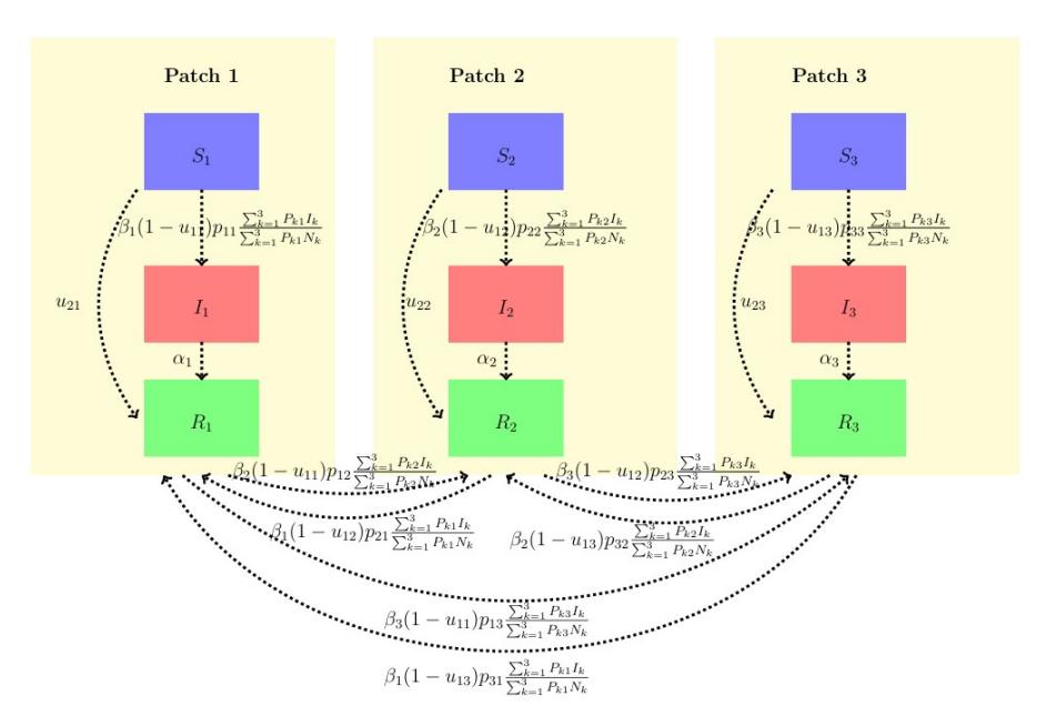
Figure 1: The proposed compartment model for 3 patches mathematically described in Equation 2.
Vaccination helps to improve the immunity of the human body. Moreover, the control measures u2i control the rate of susceptible individuals becoming infectious in patch i. When increasing the value of u2i , increase the number of vaccinated susceptible individuals and they move into the recovery class. The goal is to minimize the number of infected individuals in each patch at a minimal cost of implementation over a finite time.
Objective Functional,
\[\min_{U} J(U) = \min_{u_{1i}, u_{2i}} \int_{0}^{T} \sum_{i=1}^{n} \left( a_{i} I_{i} + \frac{b_{i}}{2} u_{1i}^{2} + \frac{c_{i}}{2} u_{2i}^{2} \right) dt.\] (3)
Equation 3 represents the objective functional, while Equation 2 represents the subject of the states. Here ai is the positive constant of the costs per treatment of the infected individual in patch i. The bi and ci are relative cost of the implementation of controls for patch i, u1i and u2i respectively. Pontryagin's Maximum Principle is the fundamental theory for solving the optimal control problem [12]. The necessary condition is defined according to Pontryagin's Maximum Principle.
Hamiltonian H is defined as, \(H = \sum_{i=1}^{n} \left( a_i I_i + \frac{b_i}{2} u_{1i}^2 + \frac{c_i}{2} u_{2i}^2 + \lambda_{1i} S_i' + \lambda_{2i} I_i' + \lambda_{3i} R_i' \right)\). There exist adjoint variables \(\lambda_{1i}\), \(\lambda_{2i}\), \(\lambda_{3i}\) where i = 0, ...n which satisfy the system of ODE in Sub-section 2.1,
\[\begin{split} \lambda'_{1i} &= -\frac{dH}{dS_i} \\ &= (\lambda_{1i} - \lambda_{2i}) \left( \sum_{j=1}^n \beta_j (1 - u_{1i}) P_{ij} \frac{\sum_{k=1}^n P_{kj} I_k}{\sum_{k=1}^n P_{kj} N_k} \right) + (\lambda_{1i} - \lambda_{3i}) u_{2i}, \\ \lambda'_{2i} &= -\frac{dH}{dI_i} \\ &= -a_i + (\lambda_{1i} - \lambda_{2i}) S_i \left( \sum_{j=1}^n \beta_j (1 - u_{1i}) P_{ij} \frac{P_{ij}}{\sum_{k=1}^n P_{kj} N_k} \right) + \alpha (\lambda_{2i} - \lambda_{3i}), \\ \lambda'_{3i} &= -\frac{dH}{dR_i} &= 0, \end{split}\] with the transversality conditions, \(\lambda_{1i}(t) = \lambda_{2i}(t) = \lambda_{3i}(t) = 0\). The optimality controls \(u_{1i}\), \(u_{2i}\) are derived by the optimality condition 4,
\[\frac{dH}{du_{1i}} = 0,\] \[\frac{dH}{du_{2i}} = 0.\] (4)
The optimality control variables \((u_{1i}^*, u_{2i}^*)\) are given by,
\[u_{1i}^* = \min \left\{ 0.8, \max \left\{ 0, \frac{(\lambda_{2i} - \lambda_{1i}) \left( \sum_{j=1}^n \beta_j \frac{\sum_{k=1}^n P_{kj} I_k}{\sum_{k=1}^n P_{kj} N_k} \right)}{b_i} \right\} \right\},\] \[u_{2i}^* = \min \left\{ 0.8, \max \left\{ 0, \frac{(\lambda_{2i} - \lambda_{3i}) S_i}{c_i} \right\} \right\}.\]
2.2. Basic reproduction number, effective reproduction number, and the final epidemic size
The basic reproductive ratio or basic reproduction number, \(R_0\) represents the significant result in the epidemiological model. \(R_0\) is the average number of infectious secondary cases when one infectious individual has originated in the susceptible population [1]. By using the Next Generation Method, \(R_0\) is computed [4]. An epidemic occurs when \(R_0 > 1\), and an endemic occurs when \(R_0 = 1\) [4]. The next generation matrix K is defined by,
\[K = -FV^{-1}\], where \(F = \begin{bmatrix} \frac{\partial f_i(x_0)}{\partial x_i} \end{bmatrix}\) and \(V = \begin{bmatrix} \frac{\partial v_i(x_0)}{\partial x_i} \end{bmatrix}\), (5)
\(f_i(x)\) be the rate of appearance of new infections in compartment i, \(v_i(x)\) is the difference between the rate of transfer of individuals into and out of compartment i. The difference of \(f_i(x) - v_i(x)\) gives the rate of change of \(x_i\). Here \(x_i\) denotes the number or proportion of individuals in the i compartment, \(x_0\) is the disease-free equilibrium point (DFE point) and i, j = 1, ..., m [4], [33]. At the point of DFE, there are no infected individuals. Then \(R_0\) is given by,
\[Ro = \max \{ eigenvalue(K) \}.\] (6)
We formulate the basic reproduction number according to the model described in Equation 2. \(f_i(I)\) and \(v_i(I)\) are defined for our model according to the Equation 5,
\[f_{i}(I) = \begin{pmatrix} S_{1}(t) \sum_{j=1}^{n} B_{j}(1 - u_{11}) P_{ij} \frac{\sum_{k=1}^{n} P_{kj} I_{k}(t)}{\sum_{k=1}^{n} P_{kj} N_{k}(t)} \\ S_{2}(t) \sum_{j=1}^{n} B_{j}(1 - u_{12}) P_{ij} \frac{\sum_{k=1}^{n} P_{kj} I_{k}(t)}{\sum_{k=1}^{n} P_{kj} N_{k}(t)} \\ \vdots \\ S_{n}(t) \sum_{j=1}^{n} B_{j}(1 - u_{1n}) P_{ij} \frac{\sum_{k=1}^{n} P_{kj} I_{k}(t)}{\sum_{k=1}^{n} P_{kj} N_{k}(t)} \end{pmatrix}, \quad -v_{i}(I) = \begin{pmatrix} \alpha I_{1} \\ \alpha I_{2} \\ \vdots \\ \alpha I_{n} \end{pmatrix}.\]
F and V are defined at the point of DFE, \(E_1 = (S_1, I_1, R_1, \dots, S_n, I_n, R_n) = (N_1, 0, 0, \dots, N_n, 0, 0)\) according to the mention in Equation 5,
\[F = \begin{pmatrix} \sum_{j=1}^{n} B_{j}(1 - u_{11}) P_{1j} \frac{P_{1j}}{\sum_{k=1}^{n} P_{kj} N_{k}(t)} & \cdots \sum_{j=1}^{n} B_{j}(1 - u_{19}) P_{1j} \frac{P_{9j}}{\sum_{k=1}^{n} P_{kj} N_{k}(t)} \\ \vdots & & \vdots \\ \sum_{j=1}^{n} B_{j}(1 - u_{19}) P_{9j} \frac{P_{9j}}{\sum_{k=1}^{n} P_{kj} N_{k}(t)} & \cdots \sum_{j=1}^{n} B_{j}(1 - u_{99}) P_{9j} \frac{P_{9j}}{\sum_{k=1}^{n} P_{kj} N_{k}(t)} \end{pmatrix},\] \[-V = \begin{pmatrix} \alpha & \cdots & 0 \\ \vdots & \ddots & \vdots \\ 0 & \cdots & \alpha \end{pmatrix}, \quad -V^{-1} = \frac{1}{\alpha} \begin{pmatrix} 1 & \cdots & 0 \\ \vdots & \ddots & \vdots \\ 0 & \cdots & 1 \end{pmatrix}.\]
Then the next generation matrix \(K \in \mathbb{R}^{9 \times 9}\),
\[K = -FV^{-1}\] \[= \frac{1}{\alpha} \begin{pmatrix} \sum_{j=1}^{n} B_{j}(1 - u_{11}) P_{1j} \frac{P_{1j}}{\sum_{k=1}^{n} P_{kj} N_{k}(t)} & \cdots \sum_{j=1}^{n} B_{j}(1 - u_{19}) P_{1j} \frac{P_{9j}}{\sum_{k=1}^{n} P_{kj} N_{k}(t)} \\ \vdots & \vdots & \vdots \\ \sum_{j=1}^{n} B_{j}(1 - u_{19}) P_{9j} \frac{P_{9j}}{\sum_{k=1}^{n} P_{kj} N_{k}(t)} & \cdots \sum_{j=1}^{n} B_{j}(1 - u_{19}) P_{9j} \frac{P_{9j}}{\sum_{k=1}^{n} P_{kj} N_{k}(t)} \end{pmatrix}.\]
\(R_0\) is given by the largest eigenvalue of K mentioned in Equation 6.
During the epidemic, a proportion of susceptible individuals become infected or immune. The effective reproduction number \((R_t)\) is an approach to capture the actual average number of secondary cases per primary case (current susceptible population) [34]. When estimating \(R_t\), it captures the impact of control measures and non-susceptible individuals in the population [35]. So the value of \(R_t\) is lower than the value of \(R_0\).
\[R_t = R_0 x, (7)\]
where \(R_0\) is the basic reproduction number and x is the fraction of the host population (that is susceptible) [36]. The effective reproduction number indicates a more sensitive value than the basic reproduction number when the outbreak is controlled by using a control measure [35]. To analyze the results, we used \(R_t\) mentioned in Equation 7.
Under the assumption that all susceptible individuals do not become infectious during an epidemic, we estimate the size of the total infected population [1]. When control measures are incorporated into the epidemic model, the final epidemic size can be used as an indicator. Furthermore, it indicates the impact of control measures [1]. The cumulative number of newly infected cases (or the final epidemic size) numerically by solving the following equation according to the model defined in Equation 1,
\[C_{i}' = S_{i} \sum_{i=1}^{n} \beta_{j} P_{ij} \frac{\sum_{k=1}^{n} P_{kj} I_{k}}{\sum_{k=1}^{n} P_{kj} N_{k}}.\]
Patch-specific final epidemic size \((C_i(t_f))\) is indicated as the cumulative number of newly infected cases in patch i. We derived the final epidemic size 8 for the model described in Equation 2 is followed as,
\[C_i' = S_i \sum_{j=1}^n \beta_j (1 - u_{1i}) P_{ij} \frac{\sum_{k=1}^n P_{kj} I_k}{\sum_{k=1}^n P_{kj} N_k}.\] (8)
3. EXPERIMENTAL RESULTS
Reported COVID-19 cases and vaccination data were collected from the Epidemiological Unit in Sri Lanka [37]. Data collected from the Ministry of Finance Sri Lanka was used to estimate the parameters associated with the costs of control measures [38]. The National Transport Commission of Sri Lanka provided mobility data. Province-wise population is on the report of Economic and Social Statistics - 2020, the Central Bank of Sri Lanka.
3.1. Fixed parameter values and estimated parameter Values
Definitions of parameters of the proposed model are shown in Table 1. According to the definitions, values are defined in Table 2.
Table 2: Parameter values.
| Symbol | Reference |
|---|---|
| \(\beta_i\) | Estimated |
| \(P_{ij}\) | Estimated |
| \(\alpha\) | \(1/10.25 days^{-1}\) [7] |
| n | 9 [32] |
In this case, n equals 9 because Sri Lanka is made up of 9 provinces. By using the number of infected individuals we estimate the transmission rate \((\beta_i)\) for each province. The nonlinear least squares (NLS) function is used to minimize the sum of the squares of the differences between the actual values and the predicted values. Python contains the optimize package in its library SciPy. To compute the NLS function by using the inbuilt function 'least_squares()'. Parameters inside the inbuild function, 'bound' and 'method' should be specified to achieve an accurate transmission rate. The 'trf' is used as a method parameter inside the 'least_squares()'. The 'trf' is used for problems with bounds [39]. Lower bounds are defined as 0.0001 and upper bounds are defined as infinity. Estimated parameter values for transmission rate \((\beta_i)\) are shown in Table 3.
Table 3: Estimated values of transmission rate \((\beta_i)\) described in Section 2.
| Symbol | Province | Value |
|---|---|---|
| \(\beta_1\) | Northern province | 0.09226 |
| \(\beta_2\) | North Western province | 0.00867 |
| \(\beta_3\) | Western province | 0.16322 |
| \(\beta_4\) | North Central province | 0.00970 |
| \(\beta_5\) | Central province | 0.00072 |
| \(\beta_6\) | Sabaragamuwa province | 0.00065 |
| \(\beta_7\) | Eastern province | 0.00442 |
| \(\beta_8\) | Uva province | 0.00010 |
| \(\beta_9\) | Southern province | 0.00026 |
In Sri Lanka, the Western province is the most commercially active and busiest province. Every day, more than a thousand of people travel into and out of the province for a variety of reasons, including work, education, and commercial activity. Moreover, it has the highest population density. The transmission rate of the Western province is estimated at high values because of the above-mentioned reasons.
The \(P_{ij}\) is constructed by available bus data in the National Transport Commission of Sri Lanka under the following assumptions due to the lack of mobility data [40], [41]. Initially, we have a number of passengers who use buses as their transportation modes province-wise. To calculate the mobility matrix, we assume that other modes of transport such as trains will contribute at proportions corresponding to their use.
3.2. Results in the absence of control measures
Before analyzing the model described in Equations 2 and 3, we analyze the spreading of the disease in the long run. As shown in Figure 4, the disease takes nearly 1000 - 1250 days (nearly 3 to 4 years) to control without any control measures. According to the following Figure 2, R0 = 1.1 which indicates a pandemic situation. A detailed representation of disease spread by using Rt with time is shown in Figure 3. After nearly 750 to 1000 days without any control strategies, Rt gradually decreases to 1.0. At that point, the disease has been controlled but does not die out.
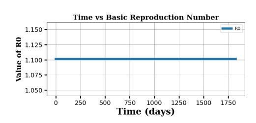
Figure 2: Basic reproduction number over time without any control measures.
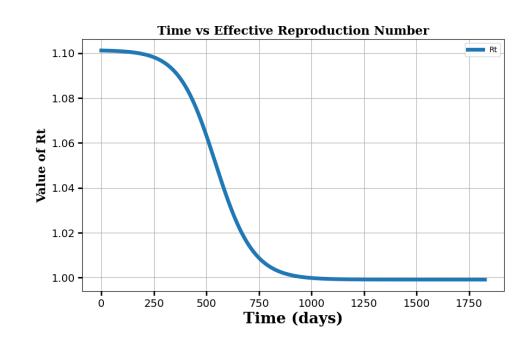
Figure 3: Effective reproduction number over time without any control measures.
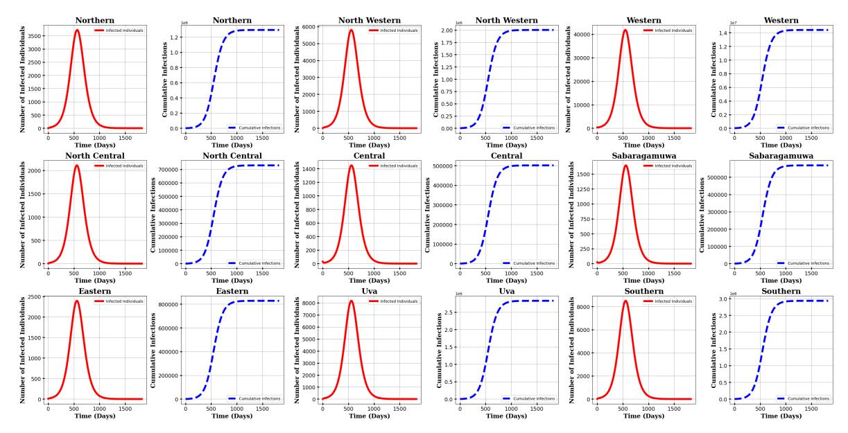
Figure 4: Red lined plot- infected individuals over time and Blue dashed-lined plot- Cumulative sum of infected individuals (Final epidemic size) over time, without any control measures respective to provinces.
For the first 450 to 700 days the spreading rate increases and when it reaches the peak value, then the spreading rate decreases. In Figure 4, red-lined plots show the infected individuals over time, and blue dashed-lined plots show the cumulative sum of infected individuals (final epidemic size) over time without any control measures respective to provinces, Northern, North Western, Western, North Central, Central, Sabaragamuwa, Eastern, Uva, and Southern. Almost 1000 days are required to control the disease, which is a long period. Disease spread negatively impacts the public health system as well as the economy of the country. The disease must be controlled within a minimum disease burden, so that the spread of the disease may be controlled.
3.3. Results in the presence of control measures separately
The need for control measures is described in sub-section 3.2. This section analyzes the behavior of disease spreading considering the control measures separately.
1) Only considering the social distancing as a control measure: The goal is to reduce the disease burden while minimizing the cost associated with the control measure (social distancing) and infectious individuals. Since COVID-19 is a novel disease, in the initial stage there are no disease-specified control measures. Taking into account the WHO guidelines, the government implements social distancing in order to reduce the disease burden.
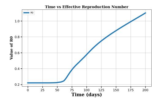
Figure 5: Effective reproduction number when social distancing is used as a control measure.
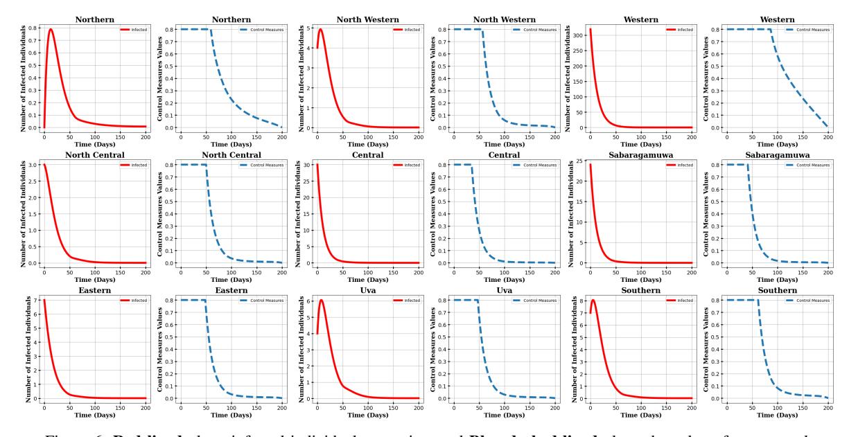
Figure 6: Red lined plot - infected individuals over time and Blue dashed-lined plot - the value of u1i control measures over time respective to provinces.
According to Figure 6, red-lined plots show the number of infected individuals over time, and blue dashedlined plots are the corresponding values of control measure (u1i). Reduce the number of infected individuals with optimal control, takes a minimum of 150 days. By implementing the maximum control measure it takes 50-80 days to control the disease burden. Due to various economic crises, 50 days of full lockdown and 50 - 80 partial lockdown are not appropriate in a low-income country such as Sri Lanka. As u1i appears to have its maximum capacity during the initial days, Rt indicates the lower value. The value of u1i gradually decreases when Rt value gradually increases, as can be observed in Figure 5. Additionally, social distancing can only control the disease burden, and it fails to reach an endemic.
2) Only considering the vaccination as a control measure: In the initial stage, the system indicates a pandemic situation. Figure 7 shows the effective reproduction number (Rt) varies with time and gradually decreases to zero. Due to the fact that vaccines contribute to the improvement of immunity within the human body, vaccinations control suspect individuals being infected individuals. The Rt represents the sensitive representation of the prediction of the secondary cases as described in the sub-section 2.2.
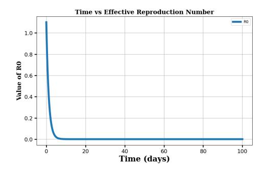
Figure 7: Effective reproduction number when vaccination is used control measure
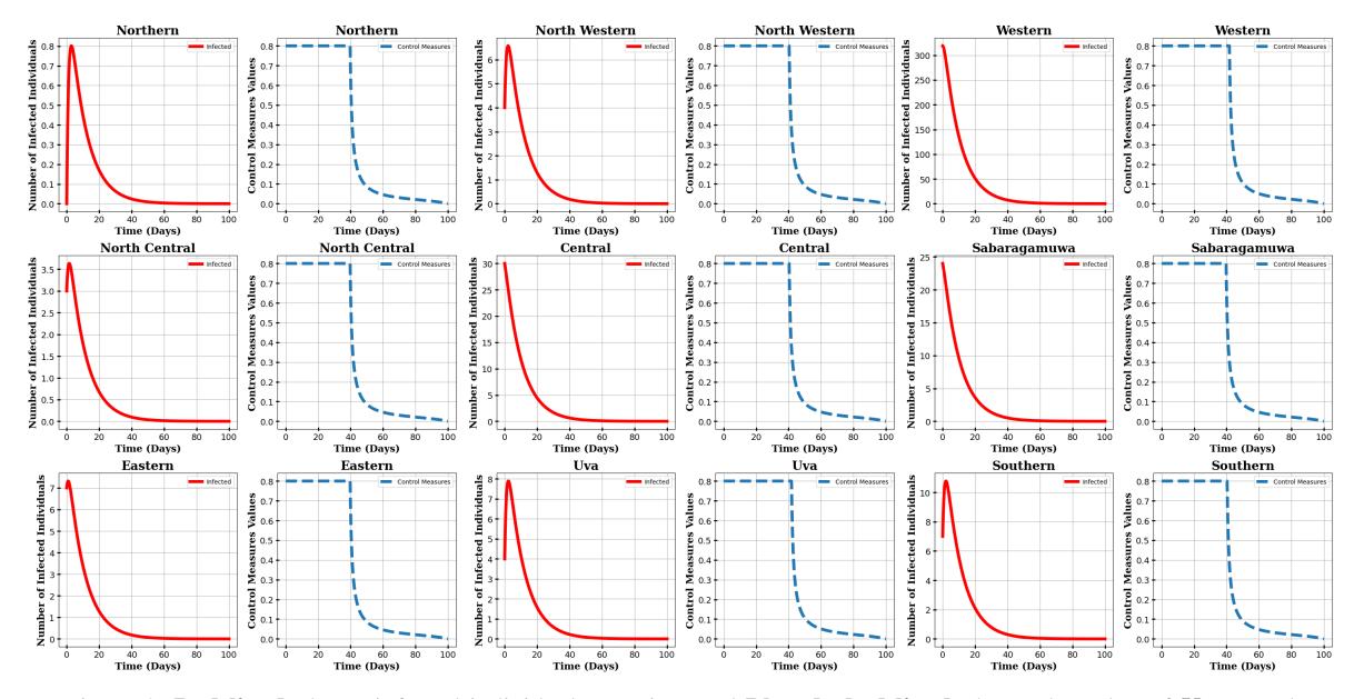
Figure 8: Red lined plots - infected individual over time and Blue dashed-lined plots - the value of U2 control measures over time respective to provinces.
The red-lined plots in Figure 8 show the number of infected individuals over time when considering the control measure. By implementing the maximum control measure it takes a maximum of nearly 40 days to control the disease burden. The corresponding value of the control measure is represented in the blue dashed-lined plots in Figure 8. To control the disease burden it takes 40 - 50 days.
Compared to the previous sub-section 3.3.1, vaccination takes less time to control the disease. Since vaccination does not disturb the lives of the general community rather than social distancing, vaccination will be the most efficient control strategy.
3.4. Results in the presence of control measures
The results are analyzed in this section using the model described in Equations 2 and 3. Sensitivity analysis is designed to capture the behavior of the disease when presenting control measures. The different relative weights for the control measures are considered in the simulation in order to identify the optimal solution that reduces the disease burden while minimizing the costs associated with control measures and infected individuals. As a result of the previous Sub-section 3.3, vaccination controls the disease burden compared to social distancing. Following Figures 9, 10, 11, 12, and 13 show the behavior of the disease spread when using the different relative cost weights for the u1i and u2i . The W1 and W2 are positive relative constants according to the u1i and u2i respectively.
1) Simulation 1: Relatively high weight for vaccination: Weight of the control measures as follows: Set W1 = 0.1 and W2 = 0.9. In the first days of the time interval, control measures are implemented at their maximum capacities. As shown in Figure 9 red-lined plots represent the infected individual over time and blue-dotted-line and orange dashed-lined plots represent the corresponding values of control measures over time with respective provinces. Under the maximum control, 30 to 40 days are taken to control the disease burden.
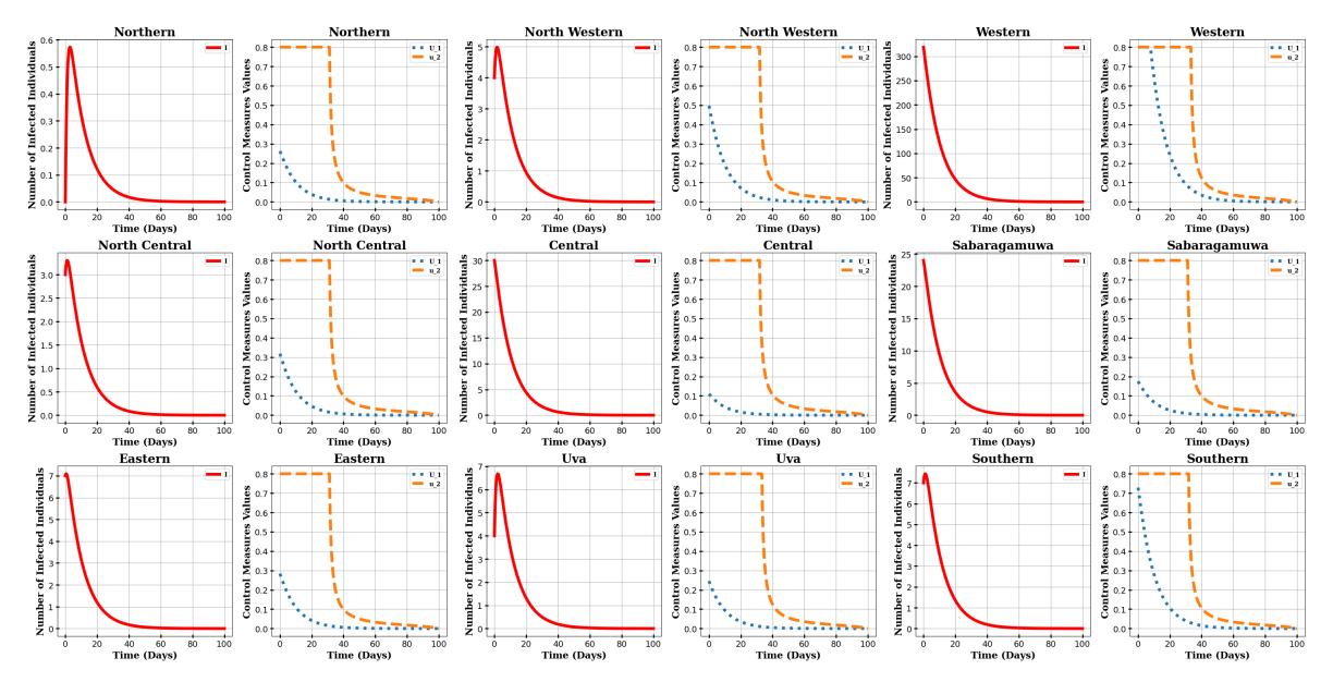
Figure 9: Red lined plot - Infected individuals over time and Blue dotted-line and Orange dashed-lined plots - Control measures over time for simulation 1 with respective provinces.
Initially, both control variables are used at their maximum capacities according to the risky provinces such as the Western province. After obtaining the control, it reduces the control values within 85 - 100 days. The u1i is used with maximum capacity in the first 10 days in Western. Southern and Northern West have to use 70% and 50% in the first days of the period respectively. Other provinces have to use less than 50% level of u1i to control the disease burden. The u2i has to be implemented at its maximum capacity first 10 days for all provinces. According to the plots Western and Southern provinces can be considered as the most critical
provinces. The weight of vaccination is higher but to reduce the disease burden vaccination could be selected as the most suitable control measure.
2) Simulation 2: Weight of social distancing as 0.3 and 0.7 as cost of vaccination: Weights for cost allocation are W1 = 0.3 and W2 = 0.7. Red, Blue- dotted, and Orange-dashed-lined plots in Figure 10 show the infected individuals, corresponding u1i and u2i overtime respectively. In this case, maximum capacities of control measures are used in between 30 - 40 days. Between the weight for the u1i and the implementing amount of u1i has an inversely proportional relationship. Only Western has to use u1i at the level of 60% in the first days of the period and other provinces implement u1i less than 30%.
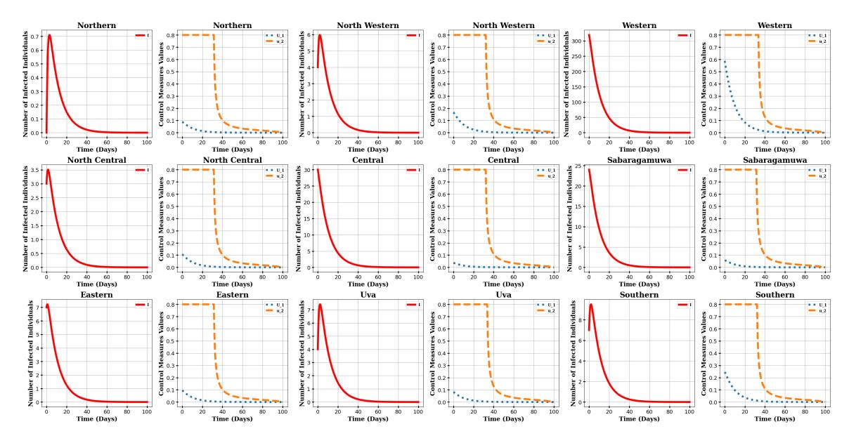
Figure 10: Red lined plot - Infected individual over time and Blue dotted-line and Orange dashed-lined plots - Control measures over time for simulation 2 with respective to provinces.
3) Simulation 3: Equal weights for both control measures: Weights are defined as equal costs for both control measures W1 = W2 = 0.5.
Red-lined plots in Figure 11 represent the infected individuals over time. The number of infected individuals is less than in the previous simulations. Blue-dotted-lined plots in Figure 11 show the control measure u1i varies with time and it has been used relatively less than the previous simulations. But in Orange-dashedlined plots in Figure 11 represent the control measure u2i and it is used relatively more than the previous simulations. The reason for the variation of weights for u1i is increasing and weights for the u2i are decreasing compared to the previous simulations.
Vaccination is used at its maximum capacity of less than 35 - 40 days. Most provinces are able to end the partial lockdown within 20 days and in risky provinces, it takes 40 days. It takes about 90-100 days to control the disease burden and that is a higher count of days comparatively with the previous simulation. The behavior of the control measures in provinces other than Western and Southern provinces is almost the same.
4) Simulation 4: Weight of social distancing as 0.7 and 0.3 as cost of vaccination: When increasing the weight of u1i , the values of the measure decrease. The total number of days to implement the control measure remains the same.
Vaccination is used for nearly 40 days with its maximum capacity to control the disease burden. Because the cost of social distancing is high, less than 50% of this control measure is used in the Western province, which was identified as a risky province in the previous simulations. Other provinces implement u1i less than 20%.to 5%. The behavior of control measures, detailed representation can be seen in blue dotted-line
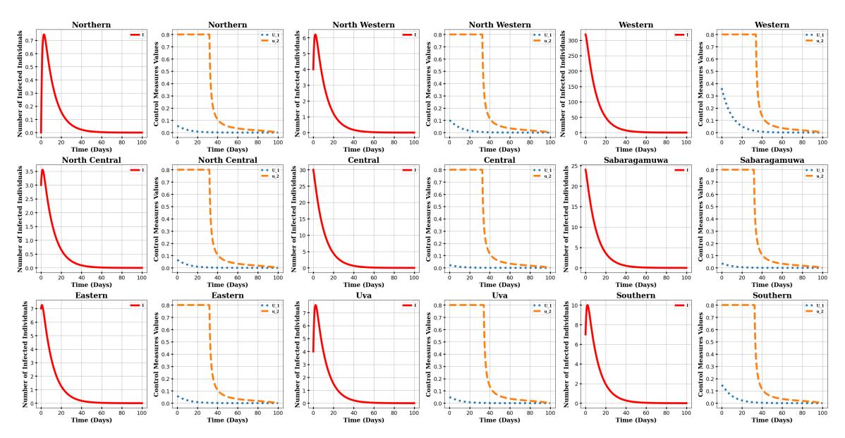
Figure 11: Red lined plot - Infected individual over time and Blue and Orange plot - Control measures over time for simulation 3 with respective to provinces.
and orange dashed-lined in Figure 12. In this simulation, vaccination is a more active control measure than the other.
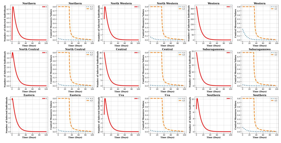
Figure 12: Red lined plot - Infected individuals over time and Blue dotted-line and Orange dashed-lined plots - Control measures over time for simulation 4 with respective to provinces.
5) Simulation 5: Relatively high weight for social distancing: The weight for u1i and u2i are equal to 0.9 and 0.1 respectively. As the result of Sub-section 3.3, we have to give more priority to vaccination than to social distancing. Infected individuals over time are shown in Figure 13 in red-lined plots and control
measures over time are shown in Figure 13 in blue-dotted and orange-dashed-lined. Nearly 40 days will be taken to control disease within all patches with maximum capacity of vaccination. Even Western province has less than 20% implementing level shown in Figure 13. The control measure in the social distance is a lower value in this situation in risky patches. In low-risk patches, the value of the control measure approaches zero due to the weight of u1i being more than the others. The behavior of both control measures all almost the same as are the provinces.
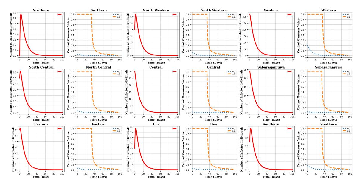
Figure 13: Red lined plot - Infected individuals over time and Blue dotted-line and Orange dashed-lined plots - Control measures over time for simulation 5 with respective to provinces.
Figure 14 shows the variation of Rt over time for simulations 1, 2, 3, 4, and 5 in subsection 3.4 respectively. The effective reproduction number Rt is interested in understanding the relationship between the control measures and the size of the disease burden. The equation of Rt in the subsection 2.2, describes the relationship between Rt and u1i are inversely proportional. When increasing the W1, the value at the initial point of Rt also increases. As a result of this, we can identify vaccination is more effective than social distancing in minimizing the disease burden and the cost of control measures.

Figure 14: Effective reproduction number over time for all simulations.
Figure 15 shows the final epidemic size for each simulation in presence control measures. According to the following Figure15, the final epidemic size of simulation 3.4.1 for each patch is higher than the other simulations. The relationship between the final epidemic size and the total cost is directly proportional and it is described in subsection 2.2. Furthermore, the final epidemic size represents the patch-specific cost value for infected individuals. Specifically, it supports decision-makers in maintaining and continuing the government and private health care system. Rt represents the overall idea of the population and the prediction of secondary cases and the final epidemic size represents the patched-specified cost value for infected individuals. Therefore, when studying meta-population or multi-patches, it is important to analyze the results of the final epidemic size.
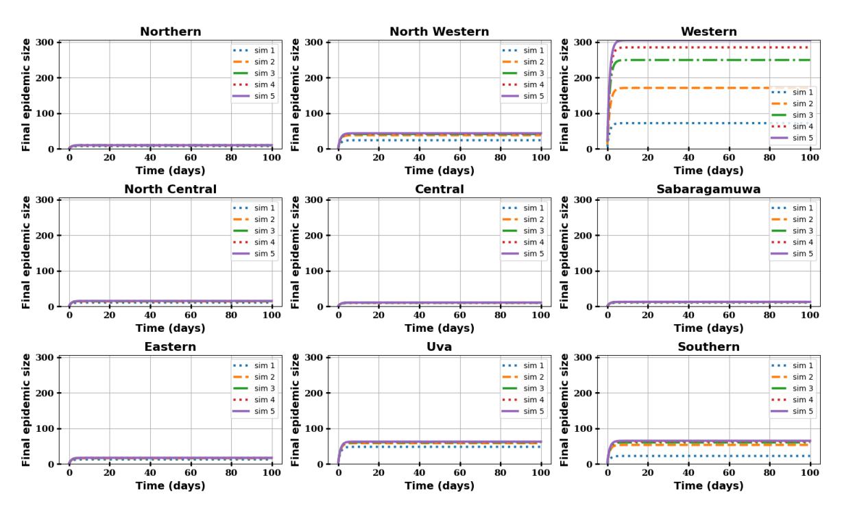
Figure 15: Final epidemic size when the presence of control measures.
4. DISCUSSION
Modeling the spread of the disease in meta-population is setting the model to real-world situations. Multiple patches are interconnected by human mobility. Mobility behaviors play a significant role in disease spread [3]. The optimal control theory is employed to identify the appropriate control strategies to reduce the size of the outbreak while minimizing the costs of implementing the control measures [4].
First, we analyze the spreading of the disease in the long run without any control measures in sub-section 3.2. According to this situation, the Rt indicates 1.1 and it is a pandemic situation. After nearly 750 to 1000 days without any control strategies, the rate of spreading disease reaches 1.0. At that point, the disease has been controlled but does not die out. In Sub-section 3.3, we analyze by considering u1i and u2i separately. Table 4 shows the summary of the results of this section.
Table 4: Summary of results when considering control measures separately.
| Control measure | Days to control | Days to use |
|---|---|---|
| the disease burden | maximum capacity | |
| Only using u1i | more than 150 | 50 days full national lockdown 50-80 partially lockdown |
| Only using u2i | 40-50 | Nearly 40 |
When considering only u1i , 30 days of national-wise lockdown and 30-80 days of full and partial lockdown are not appropriate in a low-income country such as Sri Lanka. According to the result shown in Table 4, relative to u1i , the disease can be controlled by u2i .
Then the summary of Section 3.4 is shown in Table 5. Scenarios are defined based on different weights for the cost of control measures u1i and u2i .
| W1 | W2 | Rt | Days to control | Max. days | Max. days |
|---|---|---|---|---|---|
| the disease | of u1i | of u2i | |||
| 0.1 | 0.9 | 0.5 | 85 - 100 | 10 | 30 - 40 |
| 0.3 | 0.7 | 0.6 - 0.7 | 80-100 | - | 30 - 40 |
| 0.5 | 0.5 | 0.75 - 0.8 | 90-100 | - | 35 - 40 |
| 0.7 | 0.3 | 0.85 | Nearly 100 | - | 40 |
| 0.9 | 0.1 | 0.8 - 0.9 | 100 or nearly | - | Nearly 40 |
| above days |
Table 5: Summary of results when the presence of controls measures.
The relationship between the value of W1 and the implementing level of u1i is inversely proportional. u1i contributes its maximum capacity in the first simulation, but in the last simulation, it contributes less than 20%. As a result of the Section 3, we identified u2i is controlled by the disease relatively more than the u1i . As shown in Table 5 more weight is placed on u1i , and the time taken to eliminate the disease increases. And that is also confirmed by the variation of the Rt.
The important points found in the research are summarized as follows: the multi-patch epidemic model with the human dispersal behavior approach model to be more realistic. By incorporating the optimal control theory it captured patch-specified optimal values for implementing control measures. And it helped policymakers to decide the optimal solution while minimizing the disease burden and minimizing cost. According to the analysis result, the disease can be controlled by vaccination compared to social distancing. Compared to the basic reproduction number (R0), the effective reproduction number (Rt) represents the significant result in the epidemiological model incorporated with control measures. Rt indicates the overall idea of the population and the final epidemic size represents patched-specified values. Therefore, when studying meta-population or multi-patches, it is important to analyze the results of the final epidemic size.
From these models, we provide sensitive optimal solutions regarding the COVID-19 pandemic situation in Sri Lanka. In addition to supporting the decision-making process related to continual health service in both the public and private sectors as well as maintaining the nation's economy.
5. FUTURE WORK
In this research, we formulate a multi-patch SIR model to control and reduce communicable disease outbreaks such as COVID-19 by optimizing resource allocation in Sri Lanka. The next step is to formulate a compartmental model such as SEIR, SAEIR, and SITR, which will be able to capture more complex situations as well as more real situations.