

1. Introduction
At the heart of a democratic system lies a crucial element, that is, citizen participation. This fundamental feature enables individuals to shape their nation's political landscape through active participation, such as joining political parties, voting, and participating in decision-making processes. By exercising their right to participate, citizens ensure that power remains in their hands, fostering a system of government that truly represents the will of the people. All of these activities are intended to help elect representatives for various political positions. The higher percentage of people who are enrolled in electoral lists indicates that most people are open to participating in the voting process. Additionally, it demonstrates that many people believe political participation can lead to meaningful change and transformation. However, low rates of these indicate that there are likely administrative or cultural barriers that make it difficult to register on electoral lists. These
*Corresponding Author
Received April \(8^{th}\), 2025, Revised July \(16^{th}\), 2025, Accepted for publication September \(10^{th}\), 2025. Copyright ©2025 Published by Indonesian Biomathematical Society, e-ISSN: 2549-2896, DOI:10.5614/cbms.2025.8.2.7
low percentages may also indicate a practice of political boycotting and non-registration on election lists, resulting from political and electoral corruption or a lack of trust in the political establishment. Therefore, strengthening a number of democratic metrics, such as the rate of voter registration, joining a political party, is crucial for nations looking to boost their reputation and political standing. For example, the number of people who register to vote has decreased in several Arab and African nations [7].
In a multiparty democratic system, mathematical modeling can help to understand the dynamics of electorates. Most research on political party modeling relies on statistical techniques to analyze the dynamics of two competing parties for support [7]. These studies use various statistical methods, such as descriptive statistics, inferential statistics, and predictive modeling, to understand the complexities of political competition and identify trends and patterns in voter behavior. Epidemiology and election modeling may seem like vastly different fields, but they share a common thread: the spread of influence. In epidemiology, compartmental models are used to describe the spread of infectious diseases by dividing the population into classes based on their state of the disease, such as susceptible, infected, or removed [42]. Similarly, during elections, the population can be divided into classes such as registered voters, political parties, and voting during the election. The interaction between people plays a crucial role in the voting process, much like the contagion phenomenon, where people encourage their networks to vote for a particular party. Political parties also employ direct contact strategies, such as door-to-door campaigns, to convince potential voters. This is why the epidemic approach can be effectively used to model the election process, as it captures the spread of influence and interaction between individuals [24]. The authors [21] focused on the competition between two political parties competing for the votes of undecided individuals who choose not to participate in the US federal elections. Their work explores the dynamics of this competition, shedding light on the factors that influence the decisions of these uncertain voters. The researcher in [22] examined a multiparty political system using nonlinear differential equations with a delay.
The work of [23] and [24] has enhanced our understanding of political party dynamics modeling. The article [23] employed a nonlinear model to study party growth outside conventional approaches, while [24] modeled the spread of two-party systems. The researcher [25] generalized the model proposed by Misra, considering switching between two political parties. The authors concentrated on developing mathematical models to analyze and optimize the decision-making process behind abstaining from voting during the registration of the electoral list [7]. The researchers [10] used discrete mathematical modeling to analyze electoral behavior in relation to a political party and also explored optimal control strategies to influence this behavior.
Today, one of the most famous branches of mathematical science is fractional calculus with arbitrarily fractional order [26]. Using fractional derivatives of Caputo and Riemann-Liouville, several academics have expanded this concept [1], [27]. The derivatives of Caputo and Riemann-Liouville have a singular kernel that can be interpreted as a convolution or a derivative of a convolution involving a power function [1]. Due to the singularity in the power law, Caputo and Fabrizio developed a derivative with fractional order based on the exponential function to address the issue of the singularity kernel [29], [1], [28]. They demonstrated that their derivative was appropriate for a particular group of physical problems. As their kernel was nonsingular but non-local, several problems were also raised with this derivative [1], [30]. Atangana and Baleanu presented generalized fractional derivatives in the Caputo and Riemann-Liouville senses using the Mittag-Leffler function to address the issue of the non-singular and non-local kernel. A fractional integral serves as the anti-derivative of the operators in the Atangana-Baleanu derivatives of fractional order[30], [31]. The ABC-fractional-order model has gained significant attention due to its distinctive characteristics, namely its nonsingular and nonlocal kernels. These features have made it an attractive tool for representing complex dynamical processes in various fields, including science, engineering, and others (see, for example, [43], [49], [44], [32]). In [50], a mathematical model of corruption dynamics endowed with the fractal-fractional derivative was studied.
The study of optimal control problems by fractional differential equations has various practical applications. The authors [33] created generic optimal control issues that are motivated by Riemann-Liouville fractional derivatives. The same author constructed a solid numerical framework for the mathematical model and presented comparable optimal control problems with Caputo derivatives in another study [34]. The author [16] used fractional optimal control to study a corruption model in the ABC sense. A convex incidence rate was investigated in the sense of Atangana-Baleanu and Caputo [36] in a fractional COVID-19 pandemic model that also incorporated fractional optimal control. The authors [35] created a fractional optimal control problem that takes into account public awareness and treatment for the epidemic of TB in the Caputo sense. Insight into the optimal control strategies on corruption dynamics using fractional order derivatives was studied in [17]. Fractional order modeling and optimal control of a new online game addiction model based on real data were performed [18]. The study in [20] presented a mathematical model that combines optimal control of the exponential law with the deadly combination of prostitutes and drug misuse.
We are unaware of any studies that have employed the Atangana-Baleanu fractional optimal control derivative to study the dynamics of electorates with three political parties. In the current work, we proposed an ABC fractional optimal control strategy for an awareness program that will help political parties increase the number of registered voters to vote during the election. We employed the Atangana-Baleanu and Caputo derivatives to construct the model because they have a number of desirable qualities, such as non-locality and non-singularity in their kernels, and in addition, this operator can accurately capture the crossover behavior of the model and the memory effects. The paper is structured as follows: Section (2) talks about the model foundation. Section (3) shows the analysis of the model. The optimal control strategy is explored in Section (4). Section (5) shows the numerical simulations and results. Finally, Section (6) summarizes all the results of our research.
1.1. Preliminaries
This section presents key concepts and definitions of fractional derivatives, with special attention to the Atangana-Baleanu-Caputo (ABC) framework.
Definition 1.1. According to [1], the Liouville-Caputo (LC) fractional derivative is mathematically represented as
\[{}^{C}\mathcal{D}_{\varepsilon}^{\xi}h(\varepsilon) = \frac{1}{\Gamma(1-\xi)} \int_{0}^{\varepsilon} (\varepsilon - q)^{-\xi} h'(q) dq, 0 < \xi < 1, \tag{1}\] where \(\xi\) is the fractional order.
Definition 1.2. Let \(X \in G^1(\varepsilon_1, \varepsilon_2)\), \(\varepsilon_2 > \varepsilon_1, \xi \in [0, 1]\), then, the new fractional Caputo derivative as stated in [1] is:
\[\mathcal{D}_{\varepsilon}^{\xi}(X(\varepsilon)) = \frac{\mathcal{B}(\xi)}{(1-\xi)} \int_{\varepsilon_2}^{\varepsilon} X'(q) \exp\left(-\xi\left(\frac{(\varepsilon-q)}{1-\xi}\right)\right) dq,\tag{2}\]
where \(\mathcal{B}(\xi)\) represents a normalized function, satisfying the boundary conditions \(\mathcal{B}(0) = \mathcal{B}(1) = 1\). However, if the function \(X \notin G^1(\varepsilon_1, \varepsilon_2)\) then Equation (2) has the form
\[\mathcal{D}_{\varepsilon}^{\xi}(X(\varepsilon)) = \frac{\xi \mathcal{B}(\xi)}{1 - \xi} \int_{\varepsilon_0}^{\varepsilon} (X(\varepsilon) - X(q)) \exp\left(-\xi \left(\frac{(\varepsilon - q)}{1 - \xi}\right)\right) dq. \tag{3}\]
If we let \(\pi=\frac{1-\xi}{\xi}\in[0,\infty]\) then \(\xi=\frac{1}{1+\pi}\in[0,1]\) , Equation (3) assumes the form
\[\mathcal{D}_{\varepsilon}^{\pi} X(\varepsilon) = \frac{\mathcal{B}(\pi)}{\pi} \int_{\varepsilon_2}^{\varepsilon} X'(q) \exp\left(-\left(\frac{(\varepsilon - q)}{\pi}\right)\right) dq, \mathcal{B}(0) = \mathcal{B}(\infty) = 1.\] (4)
Definition 1.3. A generalized form of the Mittag-Leffler function is given by the following expression
\[E_{\xi}(-\varepsilon^{\xi}) = \sum_{k=0}^{\infty} \frac{(-\varepsilon)^{\xi k}}{\Gamma(\xi k + 1)}.\] (5)
The Taylor series representation of \(exp(-(\varepsilon - q))\) centered at \(\varepsilon\) is given by:
\[exp(-\xi(\varepsilon - q)) = \sum_{k=0}^{\infty} \frac{(-\xi(\varepsilon - q))^k}{k!}.\] (6)
Let \(\zeta = \frac{\xi}{1-\xi}\). Substituting Equation (6) into the Caputo-Fabrizio derivative yields
\[{}_{\varepsilon_2}^{ABC} \mathcal{D}_{\varepsilon}^{\zeta} X(\varepsilon) = \frac{\mathcal{B}(\zeta)}{(1-\zeta)} \sum_{k=0}^{\infty} \frac{(-\zeta)^k}{k!} \int_{\varepsilon_2}^{\varepsilon} X'(q) (\varepsilon - q)^k dq. \tag{7}\]
To address the issue of non-locality, we derive the following expression. By modifying equation k! with \(\Gamma(\zeta k+1)\) and \((\varepsilon-q)^k\) with \((\varepsilon-q)^{\zeta k}\), we obtain:
\[{}_{\varepsilon_2}^{ABC} \mathcal{D}_{\varepsilon}^{\zeta} X(\varepsilon) = \frac{\mathcal{B}(\zeta)}{(1-\zeta)} \sum_{k=0}^{\infty} \frac{(-\zeta)^k}{\Gamma(\zeta k+1)} \int_{\varepsilon_2}^{\varepsilon} X'(q) (\varepsilon - q)^{\zeta k} dq. \tag{8}\]
As a result, [1] (2016) proposed the following derivative.
Definition 1.4. Given \(X \in G^1(\varepsilon_1, \varepsilon_2)\), \(\varepsilon_2 > \varepsilon_1\), and \(\xi \in [0, 1]\), the Atangana-Baleanu fractional derivative with a nonlocal kernel is defined as
\[{}_{\varepsilon_2}^{ABC} \mathcal{D}_{\varepsilon}^{\xi} X(\varepsilon) = \frac{\mathcal{B}(\xi)}{(1-\xi)} \int_{\varepsilon_2}^{\varepsilon} X'(q) E_{\xi} \left( -\xi \left( \frac{(\varepsilon-q)^{\xi}}{1-\xi} \right) \right) dq. \tag{9}\]
Notably, when the function X(q) is constant in Equation (9), we get zero. \(\mathcal{B}(\xi)\) retains the same properties as in the Caputo-Fabrizio case. Furthermore, the Laplace transform of Equation (9) is presented in [1] as
\[\mathcal{L}\left\{_{0}^{ABC}\mathcal{D}_{\varepsilon}^{\xi}X(\varepsilon)\right\}(r) = \frac{\mathcal{B}(\xi)}{1-\xi} \frac{r^{\xi}\mathcal{L}\left\{X(t)\right\}(r) - r^{\xi-1}X(0)}{r^{\xi} + \frac{\xi}{1-\xi}},\tag{10}\] where \(\mathcal{L}\) is the Laplace transform operator. When \(\xi = 0\), we do not recover the original function except when the function vanishes at the origin. To avoid this issue, the authors in [1] proposed the following definition.
Definition 1.5. Let \(X \in G^1(\varepsilon_1, \varepsilon_2)\), \(\varepsilon_2 > \varepsilon_1, \xi \in [0, 1]\), then, the new fractional derivative as defined in [1] is given as:
\[{}_{\varepsilon_2}^{ABR} \mathcal{D}_{\varepsilon}^{\xi} X(\varepsilon) = \frac{\mathcal{B}(\xi)}{1 - \xi} \frac{d}{d\varepsilon} \int_{\varepsilon_2}^{\varepsilon} X(q) E_{\xi} \left( -\xi \left( \frac{(\varepsilon - q)^{\xi}}{1 - \xi} \right) \right) dq, \tag{11}\]
According to [1], the Laplace transform of Equation (11) reads The Laplace transform of Equation (11) as given in [1] is:
\[\mathcal{L}\left(\left(_{0}^{ABR}\mathcal{D}_{\varepsilon}^{\xi}X(\varepsilon)\right)(r)\right) = \frac{\mathcal{B}(\xi)}{1-\xi}\frac{r^{\xi}\mathcal{L}\left(\left(X\left(\varepsilon\right)\right)\right)(r)}{r^{\xi} + \frac{\xi}{1-\varepsilon}}.\] (12)
Definition 1.6. The definition in [2], [1] gives the crucial fractional integral of the Atangana-Baleanu-Caputo derivative.
\[{}_{q}^{ABC}\mathcal{I}_{\varepsilon}^{\xi}h(\varepsilon) = \frac{(1-\xi)}{\mathcal{W}(\xi)}h(\varepsilon) + \frac{\xi}{\Gamma(\xi)\mathcal{W}(\xi)} \times \int_{q}^{\varepsilon} (\varepsilon - q)^{\xi - 1}h(q)dq. \tag{13}\]
Theorem 1.1. Given that \(X \in G^1[\varepsilon_1, \varepsilon_2]\) and \(\xi \in [0, 1]\), the subsequent result holds true [1]
\[{}_{0}^{ABC}\mathcal{D}_{\varepsilon}^{\xi}\left(X(\varepsilon)\right) = {}_{0}^{ABR}\mathcal{D}_{\varepsilon}^{\xi}\left(X(\varepsilon)\right) + G(\varepsilon). \tag{14}\]
The proof of this theorem can be found in [1].
Theorem 1.2. Let X be a continuous function in the closed interval \([\varepsilon_1, \varepsilon_2]\). Then, the following inequality holds on \([\varepsilon_1, \varepsilon_2]\).
\[\left\| {_0^{ABR}} \mathcal{D}_{\varepsilon}^{\xi} X(\varepsilon) \right\| < \frac{\mathcal{B}(\xi)}{1 - \xi} K \left\| x(\varepsilon) \right\| = \max_{\varepsilon_1 \le \varepsilon \le \varepsilon_2} \left| x(\varepsilon) \right|. \tag{15}\]
Theorem 1.3. The Atangana-Baleanu derivatives in both the Riemann and Caputo senses satisfy the Lipschitz condition. Specifically, for functions h and g, the following inequality holds, as established by [1]:
\[\left\| {}_{0}^{ABC} \mathcal{D}_{\varepsilon}^{0} h(\varepsilon) - {}_{\varepsilon}^{ABC} D_{\varepsilon}^{\xi} g(\varepsilon) \right\| \le X \left\| h(\varepsilon) - g(\varepsilon) \right\|. \tag{16}\]
2. MODEL FORMULATION
Person-to-person interaction plays a pivotal role in shaping the outcome of the election. Interactions with friends, neighbors, and family members significantly influence voting decisions, as people rely on each other to stay informed about elections. These social networks not only encourage people to cast their votes, but also persuade them to support specific parties or candidates. In essence, voting can be seen as a contagious phenomenon, where individuals "infect" others with their voting behaviors, much like an epidemic spreads [42]. We assume that a registered voter's decision is influenced by their interactions with a party member and the likelihood of accepting that party's ideology. To model this, we define variables. Eligible Voters (Q), Citizens who qualify to vote, Registered Voters (R): Citizens who have registered to vote - Major Parties: National Democratic Congress (NDC) (P1), New Patriotic Party (NPP) (P2), Minor Parties (P3): all smaller parties combined, U individual without interest to vote,N0 individual without party affiliations, and V individual who cast their votes in the political election. θ is the interaction rate of qualified Ghanaian individuals with the probability of becoming a registered voter. The remaining parameters are described in Table (2). We consider the total population under study at any time (ε) as
\[\mathcal{N}(\varepsilon) = \mathcal{Q}(\varepsilon) + \mathcal{R}(\varepsilon) + \mathcal{P}_1(\varepsilon) + \mathcal{P}_2(\varepsilon) + \mathcal{P}_3(\varepsilon) + \mathcal{U}(\varepsilon) + \mathcal{N}_0(\varepsilon) + \mathcal{V}(\varepsilon).\]
Non-affiliated individuals refer to voters who are registered but do not identify with a specific political party. They might be independent or not affiliated with any major party, whereas undecided registered voters refer to voters who have not yet decided which candidate or party they will vote for in an upcoming election. These voters may be affiliated with a party or be non-affiliated, but are uncertain about their voting decision. The study relies on the following key assumptions:
- 1) We assume that every registered voter meets the legal voting age requirement of being at least 18 years old.
- 2) We assume that each registered member is limited to joining only one political party at a time [52].
- 3) Registered voters have the flexibility to change their affiliation with their political party at any time, allowing them to update their registration to reflect changes in their political views or affiliations.
The flow chart of the model is shown in Figure (1).
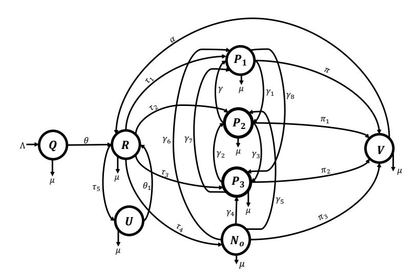
Figure 1: Flowchart of the model.
Recent studies have highlighted the importance of addressing dimensional issues in mathematical modeling [51]. Building on these efforts, we propose an ABC fractional optimal control model for the dynamics of the electorate in a multiparty democracy, described by the following system of nonlinear differential equations.
Let 0 < ξ ≤ 1 define the fractional order. The fractional model is defined as
\[\begin{array}{l} ^{ABC}D_{\varepsilon}^{\xi}\mathcal{Q} = \Lambda^{\xi} - (\theta^{\xi} + \mu^{\xi})\mathcal{Q}, \\ ^{ABC}D_{\varepsilon}^{\xi}\mathcal{R} = \theta^{\xi}\mathcal{Q} + \alpha^{\xi}\mathcal{V} + \theta_{1}^{\xi}\mathcal{U} - (\tau_{1}^{\xi}\mathcal{P}_{1} + \tau_{2}^{\xi}\mathcal{P}_{2} + \tau_{3}^{\xi}\mathcal{P}_{3} + \tau_{4}^{\xi} + \tau_{5}^{\xi} + \mu^{\xi})\mathcal{R}, \\ ^{ABC}D_{\varepsilon}^{\xi}\mathcal{P}_{1} = \tau_{1}^{\xi}\mathcal{R}\mathcal{P}_{1} + \gamma_{6}^{\xi}\mathcal{N}_{0}\mathcal{P}_{1} + \gamma^{\xi}\mathcal{P}_{2}\mathcal{P}_{1} + \gamma_{7}^{\xi}\mathcal{P}_{3}\mathcal{P}_{1} - (\pi^{\xi} + \gamma_{1}^{\xi}\mathcal{P}_{2} + \gamma_{8}^{\xi}\mathcal{P}_{3} + \mu^{\varepsilon})\mathcal{P}_{1}, \\ ^{ABC}D_{\varepsilon}^{\xi}\mathcal{P}_{2} = \tau_{2}^{\xi}\mathcal{R}\mathcal{P}_{2} + \gamma_{1}^{\xi}\mathcal{P}_{2}\mathcal{P}_{1} + \gamma_{2}^{\xi}\mathcal{P}_{3}\mathcal{P}_{2} + \gamma_{5}^{\xi}\mathcal{N}_{0}\mathcal{P}_{2} - (\pi_{1}^{\xi} + \gamma^{\xi}\mathcal{P}_{1} + \gamma_{3}^{\xi}\mathcal{P}_{3} + \mu^{\xi})\mathcal{P}_{2}, \\ ^{ABC}D_{\varepsilon}^{\xi}\mathcal{P}_{3} = \tau_{3}^{\xi}\mathcal{R}\mathcal{P}_{3} + \gamma_{3}^{\xi}\mathcal{P}_{2}\mathcal{P}_{3} + \gamma_{4}^{\xi}\mathcal{N}_{0}\mathcal{P}_{3} + \gamma_{8}^{\xi}\mathcal{P}_{1}\mathcal{P}_{3} - (\pi_{2}^{\xi} + \gamma_{7}^{\xi}\mathcal{P}_{1} + \gamma_{2}^{\xi}\mathcal{P}_{2} + \mu^{\xi})\mathcal{P}_{3}, \\ ^{ABC}D_{\varepsilon}^{\xi}\mathcal{N}_{0} = \tau_{4}^{\xi}\mathcal{R} - (\pi_{3}^{\xi} + \gamma_{4}^{\xi}\mathcal{P}_{3} + \gamma_{5}^{\xi}\mathcal{P}_{2} + \gamma_{6}^{\xi}\mathcal{P}_{1} + \mu^{\xi})\mathcal{N}_{0}, \\ ^{ABC}D_{\varepsilon}^{\xi}\mathcal{U} = \tau_{5}^{\xi}\mathcal{R} - (\theta_{1}^{\xi} + \mu^{\xi})\mathcal{U}, \\ ^{ABC}D_{\varepsilon}^{\xi}\mathcal{V} = \pi^{\xi}\mathcal{P}_{1} + \pi_{1}^{\xi}\mathcal{P}_{2} + \pi_{2}^{\xi}\mathcal{P}_{3} + \pi_{3}^{\xi}\mathcal{N}_{0} - (\alpha^{\xi} + \mu^{\xi})\mathcal{V}, \end{array} \tag{17}\]
with initial conditions Q(0) = Qo > 0, R(0) = Ro ≥ 0,P1(0) = Po ≥ 0,P2(0) = P2o ≥ 0,P3(0) = Po ≥ 0, N0(0) = N0o ≥ 0, U(0) = Uo ≥ 0, V(0) = Vo ≥ 0.
Table (2) provides a detailed description of the variable parameters used in the model.
Table 1: State variables description.
| Variable | Description |
|---|---|
| Q | Qualified Ghanaian 18 years and above |
| R | Registered voters |
| P1 | The National Democratic Congress (NDC) |
| P2 | The New Patriotic Party (NPP) |
| P3 | Combination of smallest political parties |
| U | Registered voters with no interest to vote |
| N0 | Individual with no party affiliations |
| V | Individual who cast their votes |
Table 2: Table of parameters with descriptions.
| Parameter | Description |
|---|---|
| Λ | The rate at which eligible citizens register to vote |
| µ | Death rate due to natural causes |
| τ1 | The rate at which registered voters choose to join or associate with political party P1 |
| τ2 | The rate at which registered voters choose to join or associate with political party P2 |
| τ3 | The rate at which registered voters choose to join or associate with political party P3 |
| τ4 | The rate at which registered voters decide not to join any party |
| τ5 | It refers to the proportion of registered voters who choose not to associate with any particular political party |
| π | The proportion of Party P1 member who cast their vote |
| π1 | The proportion of Party P2 member who cast their vote |
| π2 | The proportion of Party P3 member who cast their vote |
| π3 | The proportion of NO member who cast their vote |
| γ | The proportion of party P2 members who switch to party P1 |
| γ1 | The proportion of party P1 members who switch to party P2 |
| γ2 | The proportion of party P3 members who switch to party P2 |
| γ3 | The proportion of party P2 members who switch to party P3 |
| γ4 | The proportion of no party affiliation N0 members who switch to party P3 |
| γ5 | The proportion of no party affiliation N0 members who switch to party P2 |
| γ6 | The proportion of no party affiliation N0 members who switch to party P1 |
| θ1 | The proportion of undecided voters who have changed their minds to join a party |
| γ7 | The proportion of the Party P3 member who switches to the Party P1 |
| γ8 | The proportion of the Party P1 member who switches to the Party P3 |
2.1. Existence and uniqueness of solutions
The Banach fixed-point theorem is used in this section to prove the existence and uniqueness of solutions to system (17). Let A(ς) denotes a Banach space, where ς = [0, 1], and Θ = A(ς) × A(ς) × A(ς) × A(ς) ×
\[\mathcal{A}(\varsigma) \times \mathcal{A}(\varsigma) \times \mathcal{A}(\varsigma) \times \mathcal{A}(\varsigma)\] with the norm
\[\begin{split} &\|(\mathcal{Q}(\varepsilon),\mathcal{R}(\varepsilon),\mathcal{P}_{1}(\varepsilon),\mathcal{P}_{2}(\varepsilon),\mathcal{P}_{3}(\varepsilon),\mathcal{N}_{0}(\varepsilon),\mathcal{U}(\varepsilon),\mathcal{V}(\varepsilon))\|\\ &=\|\mathcal{Q}(\varepsilon)\|+\|\mathcal{R}(\varepsilon)\|+\|\mathcal{P}_{1}(\varepsilon)\|+\|\mathcal{P}_{2}(\varepsilon)\|+\|\mathcal{P}_{3}(\varepsilon)\|+\|\mathcal{N}_{0}(\varepsilon)\|+\|\mathcal{U}(\varepsilon)\|+\|\mathcal{V}(\varepsilon)\|\,, \end{split}\] where
\[\|\mathcal{Q}(\varepsilon)\| = Sup_{\varepsilon \in \varsigma} |\mathcal{Q}(\varepsilon)|, \|\mathcal{R}(\varepsilon)\| = Sup_{\varepsilon \in \varsigma} |\mathcal{R}(\varepsilon)|, \|\mathcal{P}_1(\varepsilon)\| = Sup_{\varepsilon \in \varsigma} |\mathcal{P}_1(\varepsilon)|, \|\mathcal{P}_2(\varepsilon)\| = Sup_{\varepsilon \in \varsigma} |\mathcal{P}_2(\varepsilon)|, \|\mathcal{P}_3(\varepsilon)\| = Sup_{\varepsilon \in \varsigma} |\mathcal{P}_3(\varepsilon)|, \|\mathcal{N}_O(\varepsilon)\| = Sup_{\varepsilon \in \varsigma} |\mathcal{N}_O(\varepsilon)|, \|\mathcal{U}(\varepsilon)\| = Sup_{\varepsilon \in \varsigma} |\mathcal{U}(\varepsilon)|, \|\mathcal{V}(\varepsilon)\| = Sup_{\varepsilon \in \varsigma} |\mathcal{V}(\varepsilon)|.\]
Using the fractional integral operator Atangana-Baleanu-Caputo, we transform the system (17) into
\[\text{[rumus tidak dapat ditampilkan dengan baik — lihat PDF asli]}\] (18)
Applying the Liouville-Caputo fractional derivative definition (1.6) results in the following.
\[\text{[rumus tidak dapat ditampilkan dengan baik — lihat PDF asli]}\]
where
\[\mathcal{B}_{1}(\xi, q, \mathcal{Q}(\varepsilon)) = \Lambda^{\xi} - (\theta^{\xi} + \mu^{\xi})\mathcal{Q},\] \[\mathcal{B}_{2}(\xi, q, \mathcal{R}(\varepsilon)) = \theta^{\xi}\mathcal{Q} + \alpha^{\xi}\mathcal{V} + \theta_{1}^{\xi}\mathcal{U} - (\tau_{1}^{\xi}\mathcal{P}_{1} + \tau_{2}^{\xi}\mathcal{P}_{2} + \tau_{3}^{\xi}\mathcal{P}_{3} + \tau_{4}^{\xi} + \tau_{5}^{\xi} + \mu^{\xi})\mathcal{R},\] \[\mathcal{B}_{3}(\xi, q, \mathcal{P}_{1}(\varepsilon)) = \tau_{1}^{\xi}\mathcal{R}\mathcal{P}_{1} + \gamma_{6}^{\xi}\mathcal{N}_{0}\mathcal{P}_{1} + \gamma^{\xi}\mathcal{P}_{2}\mathcal{P}_{1} + \gamma_{7}^{\xi}\mathcal{P}_{3}\mathcal{P}_{1} - (\pi^{\xi} + \gamma_{1}^{\xi}\mathcal{P}_{2} + \gamma_{8}^{\xi}\mathcal{P}_{3} + \mu^{\varepsilon})\mathcal{P}_{1},\] \[\mathcal{B}_{4}(\xi, q, \mathcal{P}_{2}(\varepsilon)) = \tau_{2}^{\xi}\mathcal{R}\mathcal{P}_{2} + \gamma_{1}^{\xi}\mathcal{P}_{2}\mathcal{P}_{1} + \gamma_{2}^{\xi}\mathcal{P}_{3}\mathcal{P}_{2} + \gamma_{5}^{\xi}\mathcal{N}_{0}\mathcal{P}_{2} - (\pi_{1}^{\xi} + \gamma^{\xi}\mathcal{P}_{1} + \gamma_{3}^{\xi}\mathcal{P}_{3} + \mu^{\xi})\mathcal{P}_{2},\] \[\mathcal{B}_{5}(\xi, q, \mathcal{P}_{3}(\varepsilon)) = \tau_{3}^{\xi}\mathcal{R}\mathcal{P}_{3} + \gamma_{3}^{\xi}\mathcal{P}_{2}\mathcal{P}_{3} + \gamma_{4}^{\xi}\mathcal{N}_{0}\mathcal{P}_{3} + \gamma_{8}^{\xi}\mathcal{P}_{1}\mathcal{P}_{3} - (\pi_{2}^{\xi} + \gamma_{7}^{\xi}\mathcal{P}_{1} + \gamma_{2}^{\xi}\mathcal{P}_{2} + \mu^{\xi})\mathcal{P}_{3},\] \[\mathcal{B}_{6}(\xi, q, \mathcal{N}_{0}(\varepsilon)) = \tau_{4}^{\xi}\mathcal{R} - (\pi_{3}^{\xi} + \gamma_{4}^{\xi}\mathcal{P}_{3} + \gamma_{5}^{\xi}\mathcal{P}_{2} + \gamma_{6}^{\xi}\mathcal{P}_{1} + \mu^{\xi})\mathcal{N}_{0},\] \[\mathcal{B}_{7}(\xi, q, \mathcal{U}(\varepsilon)) = \tau_{5}^{\xi}\mathcal{R} - (\theta_{1}^{\xi} + \mu^{\xi})\mathcal{U},\] \[\mathcal{B}_{8}(\xi, q, \mathcal{V}(\varepsilon)) = \pi^{\xi}\mathcal{P}_{1} + \pi_{1}^{\xi}\mathcal{P}_{2} + \pi_{2}^{\xi}\mathcal{P}_{3} + \pi_{3}^{\xi}\mathcal{N}_{0} - (\alpha^{\xi} + \mu^{\xi})\mathcal{V}.\]
We make the following assumption in order to support our results: \((\mathcal{M})\) For the continuous functions \((\mathcal{Q}(\varepsilon), \mathcal{Q}^*(\varepsilon), \mathcal{R}(\varepsilon), \mathcal{R}^*(\varepsilon), \mathcal{P}_1^*(\varepsilon), \mathcal{P}_1(\varepsilon), \mathcal{P}_2^*(\varepsilon), \mathcal{P}_2(\varepsilon), \mathcal{P}_3^*(\varepsilon), \mathcal{P}_3(\varepsilon), \mathcal{N}_0^*(\varepsilon), \mathcal{N}_0(\varepsilon), \mathcal{U}^*(\varepsilon), \mathcal{U}(\varepsilon), \mathcal{V}^*(\varepsilon), \mathcal{V}(\varepsilon))\) \(\in L[0,1],\)
such that \(\|\mathcal{Q}(\varepsilon)\| \leq \zeta_1\), \(\|\mathcal{R}(\varepsilon)\| \leq \zeta_2\), \(\|\mathcal{P}_1(\varepsilon)\| \leq \zeta_3\), \(\|\mathcal{P}_2(\varepsilon)\| \leq \zeta_4\), \(\|\mathcal{P}_3(\varepsilon)\| \leq \zeta_5\), \(\|\mathcal{N}_0(\varepsilon)\| \leq \zeta_6\), \(\|\mathcal{U}(\varepsilon)\| \leq \zeta_7\), \(\|\mathcal{V}(\varepsilon)\| \leq \zeta_8\).
Theorem 2.1. If assumption \((\mathcal{M})\) is correct, then the kernels \(\mathcal{B}_i, i \in \mathbb{N}^8\) meet Lipschitz requirements and are contractions as long as \(\Theta_i < 1\) for each \(i \in \mathbb{N}^8\).
Proof: Suppose that the functions \(Q(\varepsilon)\) and \(Q^*(\varepsilon)\) are paired.
\[\|\mathcal{B}_{1}(\xi,\varepsilon,\mathcal{Q}(\varepsilon)) - \mathcal{B}_{1}(\xi,\varepsilon,\mathcal{Q}^{*}(\varepsilon))\| = \|(\Lambda^{\xi} - (\theta^{\xi} + \mu^{\xi})\mathcal{Q}) - (\Lambda^{\xi} - (\theta^{\xi} + \mu^{\xi})\mathcal{Q}^{*})\|\] \[= \|-\left[(\theta^{\xi} + \mu^{\xi})\right] (\mathcal{Q}(\varepsilon) - \mathcal{Q}^{*}(\varepsilon))\|.\] (21)
Letting
\[\Theta_1 = (\theta^{\xi} + \mu^{\xi}). \tag{22}\]
Equation (21) simplifies to
\[\|\mathcal{B}_{1}(\xi,\varepsilon,\mathcal{Q}(\varepsilon)) - \mathcal{B}_{1}(\xi,\varepsilon,\mathcal{Q}^{*}(\varepsilon))\| \leq \Theta_{1} \|(\mathcal{Q}(\varepsilon) - \mathcal{Q}^{*}(\varepsilon))\|. \tag{23}\]
Similarly,
\[\begin{split} &\|\mathcal{B}_{2}(\xi,\varepsilon,\mathcal{R}(\varepsilon)) - \mathcal{B}_{2}(\xi,\varepsilon,\mathcal{R}^{*}(\varepsilon))\| \leq \Theta_{2} \|(\mathcal{R}(\varepsilon) - \mathcal{R}^{*}(\varepsilon))\| \,, \\ &\|\mathcal{B}_{3}(\xi,\varepsilon,\mathcal{P}_{1}(\varepsilon)) - \mathcal{B}_{3}(\xi,\varepsilon,\mathcal{P}_{1}^{*}(\varepsilon))\| \leq \Theta_{3} \|(\mathcal{P}_{1}(\varepsilon) - \mathcal{P}_{1}^{*}(\varepsilon))\| \,, \\ &\|\mathcal{B}_{4}(\xi,\varepsilon,\mathcal{P}_{2}(\varepsilon)) - \mathcal{B}_{4}(\xi,\varepsilon,\mathcal{P}_{2}^{*}(\varepsilon))\| \leq \Theta_{4} \|(\mathcal{P}_{2}(\varepsilon) - \mathcal{P}_{2}^{*}(\varepsilon))\| \,, \\ &\|\mathcal{B}_{5}(\xi,\varepsilon,\mathcal{P}_{3}(\varepsilon)) - \mathcal{B}_{5}(\xi,\varepsilon,\mathcal{P}_{3}^{*}(\varepsilon))\| \leq \Theta_{5} \|(\mathcal{P}_{3}(\varepsilon) - \mathcal{P}_{3}^{*}(\varepsilon))\| \,, \\ &\|\mathcal{B}_{6}(\xi,\varepsilon,\mathcal{N}_{0}(t)) - \mathcal{B}_{6}(\xi,\varepsilon,\mathcal{N}_{O}^{*}(\varepsilon))\| \leq \Theta_{6} \|(\mathcal{N}_{O}(\varepsilon) - \mathcal{N}_{O}^{*}(\varepsilon))\| \,, \\ &\|\mathcal{B}_{7}(\xi,\varepsilon,\mathcal{U}(\varepsilon)) - \mathcal{B}_{7}(\xi,\varepsilon,\mathcal{U}^{*}(\varepsilon))\| \leq \Theta_{7} \|(\mathcal{U}(\varepsilon) - \mathcal{U}^{*}(\varepsilon))\| \,, \\ &\|\mathcal{B}_{8}(\xi,\varepsilon,\mathcal{V}(\varepsilon)) - \mathcal{B}_{8}(\xi,\varepsilon,\mathcal{V}^{*}(\varepsilon))\| \leq \Theta_{8} \|(\mathcal{V}(\varepsilon) - \mathcal{Q}^{*}(\varepsilon))\| \,, \end{split}\]
where
\[\Theta_{2} = \left(\tau_{1}\zeta_{1}^{\xi} + \tau_{2}^{\xi}\zeta_{2} + \tau_{3}^{\xi}\zeta_{3} + \tau_{4}^{\xi} + \tau_{5}^{\xi} + \mu^{\xi}\right), \Theta_{3} = \left(\zeta_{2}\tau_{1} + \zeta_{6}\gamma_{6} + \zeta_{5}\gamma_{7} + \zeta_{3}\gamma - (\pi^{\xi} + \gamma_{1}^{\xi}\zeta_{3} + \gamma_{8}^{\xi}\zeta_{5} + \mu^{\xi})\right), \Theta_{4} = \left(\zeta_{2}\tau_{2} + \zeta_{3}\gamma_{1} + \zeta_{5}\gamma_{2} + \zeta_{6}\gamma_{5} - (\pi^{\xi} + \gamma^{\xi}\zeta_{3} + \gamma_{3}^{\xi}\zeta_{5} + \mu^{\xi})\right), \Theta_{5} = \left(\zeta_{2}\tau_{3} + \zeta_{4}\gamma_{3} + \zeta_{3}\gamma_{8} + \zeta_{6}\gamma_{4} - (\pi_{2}^{\xi} + \gamma_{2}^{\xi}\zeta_{4} + \gamma_{7}^{\xi}\zeta_{3} + \mu^{\xi})\right), \Theta_{6} = \left(\pi_{3}^{\xi} + \zeta_{5}\gamma_{4}^{\xi} + \zeta_{4}\gamma_{5}^{\xi} + \zeta_{6}\gamma_{6}^{\xi} + \mu^{\xi}\right), \Theta_{7} = \left(\theta_{1}^{\xi} + \mu^{\xi}\right), \Theta_{8} = \left(\alpha^{\xi} + \mu^{\xi}\right).\] (25)
Therefore, Lipschitz's condition holds. Applying system (19) again yields,
\[\text{[rumus tidak dapat ditampilkan dengan baik — lihat PDF asli]}\]
subject to the initial conditions Q(0) = Q0, R(0) = R0,P1(0) = P1,0,P2(0) = P2,0,P3(0) = P3,0, NO(0) = NO,0, U(0) = U0, V(0) = V0. The differences between consecutive terms yields
\[\text{[rumus tidak dapat ditampilkan dengan baik — lihat PDF asli]}\]
\[\begin{split} \mathcal{G}_{\mathcal{U}_n}(\varepsilon) = & \mathcal{U}_n(\varepsilon) - \mathcal{U}_{n-1}(\varepsilon) = \frac{1-\xi}{\mathbb{W}(\xi)} (\mathcal{B}_7(\xi,\varepsilon,\mathcal{U}_{n-1}(\varepsilon)) - \mathcal{B}_7(\xi,\varepsilon,\mathcal{U}_{n-2}(\varepsilon))) \\ & + \frac{\xi}{\Gamma(\xi)\mathbb{W}(\xi)} \int_0^\varepsilon (\varepsilon-q)^{\xi-1} (\mathcal{B}_7(\xi,q,\mathcal{U}_{n-1}(q)) - \mathcal{B}_7(\xi,q,\mathcal{U}_{n-2}(q))) dq, \\ \mathcal{G}_{\mathcal{V}_n}(\varepsilon) = & \mathcal{V}_n(\varepsilon) - \mathcal{V}_{n-1}(\varepsilon) = \frac{1-\xi}{\mathbb{W}(\xi)} (\mathcal{B}_8(\xi,\varepsilon,\mathcal{V}_{n-1}(\varepsilon)) - \mathcal{B}_8(\xi,\varepsilon,\mathcal{V}_{n-2}(\varepsilon))) \\ & + \frac{\xi}{\Gamma(\xi)\mathbb{W}(\xi)} \int_0^\varepsilon (\varepsilon-q)^{\xi-1} (\mathcal{B}_8(\xi,q,\mathcal{U}_{n-1}(q)) - \mathcal{B}_8(\xi,q,\mathcal{U}_{n-2}(q))) dq, \end{split}\] where
\[\text{[rumus tidak dapat ditampilkan dengan baik — lihat PDF asli]}\]
Taking into consideration equation (23) – (24) and considering
\[\begin{split} \mathcal{G}_{\mathcal{Q}_{n-1}}(\varepsilon) &= \mathcal{Q}_{n-1}(\varepsilon) - \mathcal{Q}_{n-2}(\varepsilon), \mathcal{G}_{\mathcal{R}_{n-1}}(\varepsilon) = \mathcal{R}_{n-1}(\varepsilon) - \mathcal{R}_{n-2}(\varepsilon), \mathcal{G}_{\mathcal{P}_{1,n-1}}(\varepsilon) = \mathcal{P}_{1,n-1}(\varepsilon) - \mathcal{P}_{1,n-2}(\varepsilon), \\ \mathcal{G}_{\mathcal{P}_{2,n-1}}(\varepsilon) &= \mathcal{P}_{2,n-1}(\varepsilon) - \mathcal{P}_{2,n-2}(V), \mathcal{G}_{\mathcal{P}_{3,n-1}}(\varepsilon) = \mathcal{P}_{3,n-1}(\varepsilon) - \mathcal{P}_{3,n-2}(\varepsilon), \\ \mathcal{G}_{\mathcal{N}_{O,n-1}}(\varepsilon) &= \mathcal{N}_{O,n-1}(\varepsilon) - \mathcal{N}_{O,n-2}(\varepsilon), \mathcal{G}_{\mathcal{U}_{n-1}}(\varepsilon) = \mathcal{U}_{n-1}(\varepsilon) - \mathcal{U}_{n-2}(\varepsilon), \mathcal{G}_{\mathcal{V}_{n-1}}(\varepsilon) = \mathcal{V}_{n-1}(\varepsilon) - \mathcal{V}_{n-2}(\varepsilon), \end{split}\]
\[\|\mathcal{G}_{\mathcal{Q}_{n}}(\varepsilon)\| \leq \frac{1-\xi}{\mathbb{W}(\xi)}\Theta_{1} \|\mathcal{G}_{\mathcal{Q}_{n-1}}(\varepsilon)\| \frac{\xi}{\Gamma(\xi)\mathbb{W}(\xi)}\Theta_{1} \times \int_{0}^{\varepsilon} (\varepsilon-q)^{\xi-1} \|\mathcal{G}_{\mathcal{Q}_{n-1}}(q)\| dq,\] \[\|\mathcal{G}_{\mathcal{R}_{n}}(\varepsilon)\| \leq \frac{1-\xi}{\mathbb{W}(\xi)}\Theta_{2} \|\mathcal{G}_{\mathcal{R}_{n-1}}(\varepsilon)\| \frac{\xi}{\Gamma(\xi)\mathbb{W}(\xi)}\Theta_{2} \times \int_{0}^{\varepsilon} (\varepsilon-q)^{\xi-1} \|\mathcal{G}_{\mathcal{R}_{n-1}}(q)\| dq,\] \[\|\mathcal{G}_{\mathcal{P}_{1,n}}(\varepsilon)\| \leq \frac{1-\xi}{\mathbb{W}(\xi)}\Theta_{3} \|\mathcal{G}_{\mathcal{P}_{1,n-1}}(\varepsilon)\| \frac{\xi}{\Gamma(\xi)\mathbb{W}(\xi)}\Theta_{3} \times \int_{0}^{\varepsilon} (\varepsilon-q)^{\xi-1} \|\mathcal{G}_{\mathcal{P}_{1,n-1}}(q)\| dq,\] \[\|\mathcal{G}_{\mathcal{P}_{2,n}}(\varepsilon)\| \leq \frac{1-\xi}{\mathbb{W}(\xi)}\Theta_{4} \|\mathcal{G}_{\mathcal{P}_{2,n-1}}(\varepsilon)\| \frac{\xi}{\Gamma(\xi)\mathbb{W}(\xi)}\Theta_{4} \times \int_{0}^{\varepsilon} (\varepsilon-q)^{\xi-1} \|\mathcal{G}_{\mathcal{P}_{2,n-1}}(q)\| dq,\] \[\|\mathcal{G}_{\mathcal{P}_{3,n}}(\varepsilon)\| \leq \frac{1-\xi}{\mathbb{W}(\xi)}\Theta_{5} \|\mathcal{G}_{\mathcal{P}_{3,n-1}}(\varepsilon)\| \frac{\xi}{\Gamma(\xi)\mathbb{W}(\xi)}\Theta_{5} \times \int_{0}^{\varepsilon} (\varepsilon-q)^{\xi-1} \|\mathcal{G}_{\mathcal{P}_{3,n-1}}(q)\| dq,\] \[\|\mathcal{G}_{\mathcal{N}_{O,n}}(\varepsilon)\| \leq \frac{1-\xi}{\mathbb{W}(\xi)}\Theta_{6} \|\mathcal{G}_{\mathcal{N}_{O,n-1}}(\varepsilon)\| \frac{\xi}{\Gamma(\xi)\mathbb{W}(\xi)}\Theta_{6} \times \int_{0}^{\varepsilon} (\varepsilon-q)^{\xi-1} \|\mathcal{G}_{\mathcal{N}_{0,n-1}}(q)\| dq,\] \[\|\mathcal{G}_{\mathcal{U}_{n}}(\varepsilon)\| \leq \frac{1-\xi}{\mathbb{W}(\xi)}\Theta_{7} \|\mathcal{G}_{\mathcal{U}_{n-1}}(\varepsilon)\| \frac{\xi}{\Gamma(\xi)\mathbb{W}(\xi)}\Theta_{7} \times \int_{0}^{\varepsilon} (\varepsilon-q)^{\xi-1} \|\mathcal{G}_{\mathcal{U}_{n-1}}(q)\| dq,\] \[\|\mathcal{G}_{\mathcal{V}_{n}}(\varepsilon)\| \leq \frac{1-\xi}{\mathbb{W}(\xi)}\Theta_{8} \|\mathcal{G}_{\mathcal{Q}_{n-1}}(\varepsilon)\| \frac{\xi}{\Gamma(\xi)\mathbb{W}(\xi)}\Theta_{8} \times \int_{0}^{\varepsilon} (\varepsilon-q)^{\xi-1} \|\mathcal{G}_{\mathcal{V}_{n-1}}(q)\| dq.\]
Theorem 2.2. The system (17) has a unique solution for ξ ∈ [0, 1] subject to the condition 1−ξ W(ξ)Θi + Θi W(ξ)Γ(ξ) ni < 1, i = 1, 2, 3, 4, 5, 6, 7, 8 holds [3].
Proof: Since Q(ε), R(ε),P1(ε),P2(ε),P3(ε), NO(ε), U(ε), V(ε) are bounded functions and Equation
(21) - (24) holds. In a recurring manner (28) reaches
\[\|\mathcal{G}_{\mathcal{Q}_{n}}(\varepsilon)\| \leq \|\mathcal{Q}_{0}(\varepsilon)\| \left(\frac{1-\xi}{\mathbb{W}(\xi)}\Theta_{1} + \frac{1}{\Gamma(\xi)\mathbb{W}(\xi)}\Theta_{1}\right)^{n},\] \[\|\mathcal{G}_{\mathcal{R}_{n}}(\varepsilon)\| \leq \|\mathcal{R}_{0}(\varepsilon)\| \left(\frac{1-\xi}{\mathbb{W}(\xi)}\Theta_{2} + \frac{1}{\Gamma(\xi)\mathbb{W}(\xi)}\Theta_{2}\right)^{n},\] \[\|\mathcal{G}_{\mathcal{P}_{1,n}}(\varepsilon)\| \leq \|\mathcal{P}_{1,0}(\varepsilon)\| \left(\frac{1-\xi}{\mathbb{W}(\xi)}\Theta_{3} + \frac{1}{\Gamma(\xi)\mathbb{W}(\xi)}\Theta_{3}\right)^{n},\] \[\|\mathcal{G}_{\mathcal{P}_{2,n}}(\varepsilon)\| \leq \|\mathcal{P}_{2,0}(\varepsilon)\| \left(\frac{1-\xi}{\mathbb{W}(\xi)}\Theta_{4} + \frac{1}{\Gamma(\xi)\mathbb{W}(\xi)}\Theta_{4}\right)^{n},\] \[\|\mathcal{G}_{\mathcal{P}_{3,n}}(\varepsilon)\| \leq \|\mathcal{P}_{3,0}(\varepsilon)\| \left(\frac{1-\xi}{\mathbb{W}(\xi)}\Theta_{5} + \frac{1}{\Gamma(\xi)\mathbb{W}(\xi)}\Theta_{5}\right)^{n},\] \[\|\mathcal{G}_{\mathcal{N}_{O,n}}(\varepsilon)\| \leq \|\mathcal{N}_{O,0}(\varepsilon)\| \left(\frac{1-\xi}{\mathbb{W}(\xi)}\Theta_{6} + \frac{1}{\Gamma(\xi)\mathbb{W}(\xi)}\Theta_{6}\right)^{n},\] \[\|\mathcal{G}_{\mathcal{U}_{n}}(\varepsilon)\| \leq \|\mathcal{U}_{0}(\varepsilon)\| \left(\frac{1-\xi}{\mathbb{W}(\xi)}\Theta_{7} + \frac{1}{\Gamma(\xi)\mathbb{W}(\xi)}\Theta_{7}\right)^{n},\] \[\|\mathcal{G}_{\mathcal{V}_{n}}(\varepsilon)\| \leq \|\mathcal{V}_{0}(\varepsilon)\| \left(\frac{1-\xi}{\mathbb{W}(\xi)}\Theta_{8} + \frac{1}{\Gamma(\xi)\mathbb{W}(\xi)}\Theta_{8}\right)^{n},\]
and
\(\text{[rumus tidak dapat ditampilkan dengan baik — lihat PDF asli]}\)
\[\|\mathcal{Q}_{n+j}(\varepsilon) - \mathcal{Q}_{n}(\varepsilon)\| \leq \sum_{i=n+1}^{n+j} \mathcal{H}_{1}^{i} = \frac{\mathcal{H}_{1}^{n+1} - \mathcal{H}_{1}^{n+j+1}}{1 - \mathcal{H}_{1}},\] \[\|\mathcal{R}_{n+j}(\varepsilon) - \mathcal{R}_{n}(\varepsilon)\| \leq \sum_{i=n+1}^{n+j} \mathcal{H}_{2}^{i} = \frac{\mathcal{H}_{2}^{n+1} - \mathcal{H}_{2}^{n+j+1}}{1 - \mathcal{H}_{2}},\] \[\|\mathcal{P}_{1,n+j}(\varepsilon) - \mathcal{P}_{1,n}(\varepsilon)\| \leq \sum_{i=n+1}^{n+j} \mathcal{H}_{3}^{i} = \frac{\mathcal{H}_{3}^{n+1} - \mathcal{H}_{3}^{n+j+1}}{1 - \mathcal{H}_{3}},\] \[\|\mathcal{P}_{2,n+j}(\varepsilon) - \mathcal{P}_{2,n}(\varepsilon)\| \leq \sum_{i=n+1}^{n+j} \mathcal{H}_{4}^{i} = \frac{\mathcal{H}_{4}^{n+1} - \mathcal{H}_{4}^{n+j+1}}{1 - \mathcal{H}_{4}},\] \[\|\mathcal{P}_{3,n+j}(\varepsilon) - \mathcal{P}_{3,n}(\varepsilon)\| \leq \sum_{i=n+1}^{n+j} \mathcal{H}_{5}^{i} = \frac{\mathcal{H}_{5}^{n+1} - \mathcal{H}_{5}^{n+j+1}}{1 - \mathcal{H}_{5}},\] \[\|\mathcal{N}_{O,n+j}(\varepsilon) - \mathcal{N}_{O,n}(\varepsilon)\| \leq \sum_{i=n+1}^{n+j} \mathcal{H}_{6}^{i} = \frac{\mathcal{H}_{6}^{n+1} - \mathcal{H}_{6}^{n+j+1}}{1 - \mathcal{H}_{6}},\] \[\|\mathcal{U}_{n+j}(\varepsilon) - \mathcal{U}_{n}(\varepsilon)\| \leq \sum_{i=n+1}^{n+j} \mathcal{H}_{7}^{i} = \frac{\mathcal{H}_{7}^{n+1} - \mathcal{H}_{7}^{n+j+1}}{1 - \mathcal{H}_{7}},\] \[\|\mathcal{V}_{n+j}(\varepsilon) - \mathcal{V}_{n}(\varepsilon)\| \leq \sum_{i=n+1}^{n+j} \mathcal{H}_{8}^{i} = \frac{\mathcal{H}_{8}^{n+1} - \mathcal{H}_{8}^{n+j+1}}{1 - \mathcal{H}_{8}},\] where \(\mathcal{H}_i = \frac{1-\xi}{\mathbb{W}(\xi)}\Theta_i + \frac{1}{\mathbb{W}(\xi)\Gamma(\xi)}\Theta_i < 1\). Therefore, a unique solution exists for the system (17).
2.2. Hyers-Ulam Stability
Definition 2.1. Atangana-Baleanu fractional derivative system (17) is said to be Hyers-Ulam stable if constants \(\hbar_i < 0, i \in \mathbb{N}^8\) matching the following conditions exist for any \(\bar{\pi}_i > 0, i \in \mathbb{N}^8\)
\[\text{[rumus tidak dapat ditampilkan dengan baik — lihat PDF asli]}\] and there exist \(\{\mathcal{Q}(\varepsilon), \mathcal{R}(\varepsilon), \mathcal{P}_1(\varepsilon), \mathcal{P}_2(\varepsilon), \mathcal{P}_3(\varepsilon), \mathcal{N}_O(\varepsilon), \mathcal{U}(\varepsilon)\}, \mathcal{V}(\varepsilon), \text{ where }\)
\[\text{[rumus tidak dapat ditampilkan dengan baik — lihat PDF asli]}\]
such that
\[\begin{aligned} & \left| \mathcal{Q}(\varepsilon) - \overset{\bullet}{\mathcal{Q}}(\varepsilon) \right| \leq \zeta_{1}\bar{\pi}_{1}, \left| \mathcal{R}(\varepsilon) - \overset{\bullet}{\mathcal{R}}(\varepsilon) \right| \leq \zeta_{2}\bar{\pi}_{2}, \left| \mathcal{P}_{1}(\varepsilon) - \overset{\bullet}{\mathcal{P}_{1}}(\varepsilon) \right| \leq \zeta_{3}\bar{\pi}_{3}, \left| \mathcal{P}_{2}(\varepsilon) - \overset{\bullet}{\mathcal{P}_{2}}(\varepsilon) \right| \leq \zeta_{4}\bar{\pi}_{4}, \\ & \left| \mathcal{P}_{3}(\varepsilon) - \overset{\bullet}{\mathcal{P}_{3}}(\varepsilon) \right| \leq \zeta_{5}\bar{\pi}_{5}, \left| \mathcal{N}_{O}(\varepsilon) - \overset{\bullet}{\mathcal{N}_{O}}(\varepsilon) \right| \leq \zeta_{6}\bar{\pi}_{6}, \left| \mathcal{U}(\varepsilon) - \overset{\bullet}{\mathcal{U}}(\varepsilon) \right| \leq \zeta_{7}\bar{\pi}_{7}, \left| \mathcal{V}(\varepsilon) - \overset{\bullet}{\mathcal{V}}(\varepsilon) \right| \leq \zeta_{8}\bar{\pi}_{8}. \end{aligned}\]
MODEL ANALYSIS
3.1. Solution Positivity Analysis
Theorem 3.1. The solution \(\mathcal{F} = (\mathcal{Q}(\varepsilon), \mathcal{R}(\varepsilon), \mathcal{P}_1(\varepsilon), \mathcal{P}_2(\varepsilon), \mathcal{P}_3(\varepsilon), \mathcal{N}_O(\varepsilon), \mathcal{U}(\varepsilon), \mathcal{V}(\varepsilon))\) to the model (17) for all \(\varepsilon > 0\), provided that the initial conditions \((\mathcal{Q}(0), \mathcal{R}(0), \mathcal{P}_1(0), \mathcal{P}_2(0), \mathcal{P}_3(0), \mathcal{N}_O(0), \mathcal{U}(0), \mathcal{V}(0))\) are nonnegative and \(\xi\) lies in the interval (0,1].
Proof: Following the approach presented in [37], we can establish the existence and uniqueness of solutions to the system (17) in the time interval \((0, \infty)\). Furthermore, we must verify that the nonnegative region \(\mathcal{F}\) is positively invariant. An examination of the model (17) yields the following result
\[{}_{0}^{ABC}\mathcal{D}_{\varepsilon}^{\xi}\mathcal{Q}|_{\mathcal{Q}=0} = \Lambda^{\xi} > 0,\] \[{}_{0}^{ABC}\mathcal{D}_{\varepsilon}^{\xi}\mathcal{R}|_{\mathcal{R}=0} = \theta^{\xi}\mathcal{Q} + \alpha^{\xi}\mathcal{V} + \theta_{1}^{\xi}\mathcal{U} > 0,\] \[{}_{0}^{ABC}\mathcal{D}_{\varepsilon}^{\xi}\mathcal{P}_{1}|_{\mathcal{P}_{1}=0} > 0,\] \[{}_{0}^{ABC}\mathcal{D}_{\varepsilon}^{\xi}\mathcal{P}_{2}|_{\mathcal{P}_{2}=0} > 0,\] \[{}_{0}^{ABC}\mathcal{D}_{\varepsilon}^{\xi}\mathcal{P}_{3}|_{\mathcal{P}_{3}=0} > 0,\] \[{}_{0}^{ABC}\mathcal{D}_{\varepsilon}^{\xi}\mathcal{P}_{3}|_{\mathcal{N}_{0}=0} = \tau_{4}^{\xi}\mathcal{R} > 0,\] \[{}_{0}^{ABC}\mathcal{D}_{\varepsilon}^{\xi}\mathcal{N}_{0}|_{\mathcal{N}_{0}=0} = \tau_{5}^{\xi}\mathcal{R} > 0,\] \[{}_{0}^{ABC}\mathcal{D}_{\varepsilon}^{\xi}\mathcal{U}|_{\mathcal{U}=0} = \pi^{\xi}\mathcal{P}_{1} + \pi_{1}^{\xi}\mathcal{P}_{2} + \pi_{2}^{\xi}\mathcal{P}_{3} + \pi_{3}\mathcal{N}_{0} > 0.\] \[(33)\]
If \(((\mathcal{Q}(0), \mathcal{R}(0), \mathcal{P}_1(0), \mathcal{P}_2(0), \mathcal{P}_3(0), \mathcal{N}_O(0), \mathcal{U}(0), \mathcal{V}(0)) \in \mathbb{R}^8_+\), then according to equation (17) and Remark 3.2 in [15], the solution
\[(\mathcal{Q}(\varepsilon), \mathcal{R}(\varepsilon), \mathcal{P}_1(\varepsilon), \mathcal{P}_2(\varepsilon), \mathcal{P}_3(\varepsilon), \mathcal{N}_O(\varepsilon), \mathcal{U}(\varepsilon), \mathcal{V}(\varepsilon)) \in \mathbb{R}^8_+\]
cannot escape the hyperplanes of \(\mathcal{Q}=0, \mathcal{R}=0, \mathcal{P}_1=0, \mathcal{P}_2=0, \mathcal{P}_3=0, \mathcal{N}_0=0, \mathcal{U}=0,\) and \(\mathcal{V}=0.\) Also, in each hyperplane, the vector field points into \(\mathcal{F}_+\); i.e. the solution will remain in the region \(\mathcal{F}_+\). Therefore, this region is a positive invariant set.
1) Invariant Set:
Theorem 3.2. Let \(\text{[rumus tidak dapat ditampilkan dengan baik — lihat PDF asli]}\). The feasible solution set \(\left\{ \mathcal{Q}(\varepsilon), \mathcal{R}(\varepsilon), \mathcal{P}_1(\varepsilon), \mathcal{P}_2(\varepsilon), \mathcal{P}_3(\varepsilon), \mathcal{N}_O(\varepsilon), \mathcal{U}(\varepsilon), \mathcal{V}(\varepsilon) \right\} \in \mathbf{R}_+^8 = \mathbb{R}_+^8\) of the equation of the model system 17 enters and is bounded in the region \(\Omega\).
Proof: By summing all equations in model (17), we obtain the fractional derivative of the total population, which is
\[\begin{array}{l} {}^{ABC}_{0}\mathcal{D}_{\varepsilon}^{\xi}N(\varepsilon) = {}^{ABC}_{0}\mathcal{D}_{\varepsilon}^{\xi}\mathcal{Q}(\varepsilon) + {}^{ABC}_{0}\mathcal{D}_{\varepsilon}^{\xi}\mathcal{R}(\varepsilon) + {}^{ABC}_{0}\mathcal{D}_{\varepsilon}^{\xi}\mathcal{P}_{1}(\varepsilon) + {}^{ABC}_{0}\mathcal{D}_{\varepsilon}^{\xi}\mathcal{P}_{2}(\varepsilon) + {}^{ABC}_{0}\mathcal{D}_{\varepsilon}^{\xi}\mathcal{P}_{3}(\varepsilon) \\ &+ {}^{ABC}_{0}\mathcal{D}_{\varepsilon}^{\xi}\mathcal{N}_{O}(\varepsilon) + {}^{ABC}_{0}\mathcal{D}_{\varepsilon}^{\xi}\mathcal{U}(\varepsilon) + {}^{ABC}_{0}\mathcal{D}_{\varepsilon}^{\xi}\mathcal{V}(\varepsilon). \end{array}\] \[\begin{array}{l} {}^{ABC}_{0}\mathcal{D}_{\varepsilon}^{\xi}N(\varepsilon) = \Lambda^{\xi} - \mu^{\xi}(\mathcal{Q} + \mathcal{R} + \mathcal{P}_{1} + \mathcal{P}_{2} + \mathcal{P}_{3} + \mathcal{N}_{O} + \mathcal{U} + \mathcal{V}) \\ {}^{ABC}_{0}\mathcal{D}_{\varepsilon}^{\xi}N(\varepsilon) = \Lambda^{\xi} - \mu^{\xi}N. \end{array}\] (34)
Applying the Laplace transform to equation (34) yields
\[L[_0^{ABC} \mathcal{D}_{\varepsilon}^{\xi} N(\varepsilon)][s] + L[\mu^{\xi} N(\varepsilon)[s]] \ge L\{\Lambda^{\xi}\}[s].\]
In line with the approach presented in [46], equation (34) takes the form
\[L[_0^{ABC} \mathcal{D}_{\varepsilon}^{\xi} N(\varepsilon)][s] + L[\mu N(\varepsilon)[s]] \ge L\{\Lambda^{\xi}\}[s]\] \[s^{\xi} N(s) - s^{\xi-1} N(0) + \mu^{\xi} N(s) \ge \frac{\Lambda^{\xi}}{s}\] \[N(s)(s^{\xi} + \mu) \ge \frac{\Lambda^{\xi}}{s} + s^{\xi-1} N(0).\]
Hence, take \(s^{\xi-1}N(0)=0\) at \(\varepsilon=0\).
\[N(s) \ge \frac{\Lambda^{\xi} s^{-1}}{s^{\xi} + \mu^{\xi}}\]
Applying inverse Laplace transform techniques to N(s) and incorporating the Mittag-Leffler function, we find
\[N(\varepsilon) \le \Lambda^{\xi} L^{-1} \left\{ \frac{s^{-1}}{s^{\xi} + \mu^{\xi}} \right\}\] \[\le \Lambda^{\xi} \varepsilon^{\xi} \mathbb{E}_{\xi, \xi+1} (-\mu \varepsilon^{\xi})\] \[\le \frac{\Lambda^{\xi}}{\mu^{\xi}} \left[ 1 - \mathbb{E}_{\xi} (-\mu \varepsilon^{\xi}) \right].\]
As a result, we obtain
\[N(\varepsilon) \le \frac{\Lambda^{\xi}}{\mu^{\xi}} \left[ 1 - \mathbb{E}_{\xi}(-\mu^{\xi} \varepsilon^{\xi}) \right]. \tag{35}\]
For \(\mu>0\), as \(\varepsilon\) becomes infinitely large, \(N(\varepsilon)\) converges to the non-negative value \(\frac{\Lambda^{\xi}}{\mu^{\xi}}\). Hence, we establish the bound \(0\leq N(\varepsilon)\leq \frac{\Lambda^{\xi}}{\mu^{\xi}}\).
\[\Omega = \left\{ \begin{array}{l} \mathcal{Q}(\varepsilon), \mathcal{R}(\varepsilon), \mathcal{P}1(\varepsilon), \mathcal{P}_2(\varepsilon), \mathcal{P}_3(\varepsilon), \mathcal{N}_O(\varepsilon), \mathcal{U}(\varepsilon), \mathcal{V}(\varepsilon)) \in \mathbf{R}_+^8 \\ \mathcal{Q}(\varepsilon) + \mathcal{R}(\varepsilon) + \mathcal{P}_1(\varepsilon) + \mathcal{P}_2(\varepsilon) + \mathcal{P}_3(\varepsilon) + \mathcal{N}_O(\varepsilon) + \mathcal{U}(\varepsilon) + \mathcal{V}(\varepsilon) \leq \frac{\Lambda^{\xi}}{\mu^{\xi}} \end{array} \right\}\]
indicating a positively invariant set. This implies that the solution of the model (17) is stable and bounded.
2) Equilibrium points: In this section, we analyze the equilibrium points of our model. Political Party Endemic Equilibrium (PPEE) refers to the existence of political parties within the population. Political Party-Free Equilibrium (PPFE) refers to the absence of political parties in the population, where \(\mathcal{P}_1 = \mathcal{P}_2 = \mathcal{P}_3 = 0\). The political party free equilibrium \((\mathcal{Q}_0, \mathcal{R}_0, \mathcal{P}_{1,0}, \mathcal{P}_{2,0}, \mathcal{P}_{3,0}, \mathcal{N}_{0,O}, \mathcal{U}_0, \mathcal{V}_0)\) is given as
\[\begin{split} \mathcal{Q}_0 = & \frac{\Lambda^\xi}{(\theta^\xi + \mu^\xi)}, \\ \mathcal{R}_0 = & \frac{(\mu^\xi + \pi^\xi)(\alpha^\xi + \mu^\xi)(\theta_1^\xi + \mu^\xi)\theta^\xi\Lambda^\xi}{(\theta^\xi + \mu^\xi)\left((\mu^\xi + \pi^\xi)(\alpha^\xi + \mu^\xi)(\theta_1^\xi + \mu^\xi) - (\mu^\xi + \pi^\xi)(\alpha^\xi + \mu^\xi)\tau_5^\xi\theta_1^\xi - \alpha^\xi(\theta_1^\xi + \mu^\xi)\tau_4^\xi\pi_3^\xi\right)}, \\ \mathcal{P}_{1.0} = & 0, \\ \mathcal{P}_{2.0} = & 0, \\ \mathcal{P}_{3.0} = & 0, \\ \mathcal{N}_{0.0} = & \frac{(\mu^\xi + \pi^\xi)(\alpha^\xi + \mu^\xi)\theta^\xi\Lambda^\xi\tau_4^\xi}{(\theta^\xi + \mu^\xi)\left((\mu^\xi + \pi^\xi)(\alpha^\xi + \mu^\xi)(\theta_1^\xi + \mu^\xi) - (\mu^\xi + \pi^\xi)(\alpha^\xi + \mu^\xi)\tau_5^\xi\theta_1^\xi - \alpha^\xi(\theta_1^\xi + \mu^\xi)\tau_4^\xi\pi_3^\xi\right)}, \\ \mathcal{U}_0 = & \frac{(\mu^\xi + \pi^\xi)(\alpha^\xi + \mu^\xi)(\theta^\xi + \mu^\xi) - (\mu^\xi + \pi^\xi)(\alpha^\xi + \mu^\xi)\tau_5^\xi\theta_1^\xi - \alpha^\xi(\theta_1^\xi + \mu^\xi)\tau_4^\xi\pi_3^\xi\right)}{(\theta^\xi + \mu^\xi)\left\{(\mu^\xi + \pi^\xi)(\alpha^\xi + \mu^\xi)(\theta_1^\xi + \mu^\xi)(\tau_4^\xi + \tau_5^\xi + \mu^\xi) - (\mu^\xi + \pi^\xi)(\alpha^\xi + \mu^\xi)\tau_5^\xi\theta_1^\xi - \alpha^\xi(\theta_1^\xi + \mu^\xi)\tau_4^\xi\pi_3^\xi\right\}}, \\ \mathcal{V}_0 = & \frac{(\theta_1^\xi + \mu^\xi)(\theta^\xi\Lambda^\xi\tau_4^\xi\pi_3^\xi)}{(\theta^\xi + \mu^\xi)\left\{(\mu^\xi + \pi^\xi)(\alpha^\xi + \mu^\xi)(\theta_1^\xi + \mu^\xi)(\tau_4^\xi + \tau_5^\xi + \mu^\xi) - (\mu^\xi + \pi^\xi)(\alpha^\xi + \mu^\xi)\tau_5^\xi\theta_1^\xi - \alpha^\xi(\theta_1^\xi + \mu^\xi)\tau_4^\xi\pi_3^\xi\right\}}. \end{split}\]
We found that democracy can function without political parties, known as nonpartisan or no-party democracy. This system involves regular elections where the candidates are not affiliated with specific parties. This means that candidates run independently and registered voters choose based on individual merit rather than party affiliation. In nonpartisan democracies, elections often focus on issues rather than party politics. Sometimes, electioneering and even speaking about candidates may be discouraged to prevent influencing others' decisions or creating tension [53]. This type of democracy can be seen in countries such as Micronesia, Tuvalu, Oman, and Palau, where candidates run independently without affiliation with any party [53].
The basic reproduction number plays a key role in shaping the growth of the popularity of a political party among voters. It represents the average number of registered voters that a political party can influence in a fully susceptible population. This number serves as a threshold, calculated using the voter model, denoted by \(\mathcal{R}_0\), which corresponds to the maximum eigenvalue of the next generation matrix [48]. In essence, the basic reproduction number assesses the potential spread of a political party's influence. The formulas incorporate two key components: \(\mathcal{F}\), representing new registered voters joining the party, and \(\mathcal{V}\), representing registered voters leaving the party. This delicate balance between acquisition and loss of supporters ultimately determines
\[\mathcal{F} = \begin{pmatrix} \tau_1^{\xi} \mathcal{R} \mathcal{P}_1 + \gamma_6^{\xi} \mathcal{N}_0 \mathcal{P}_1 + \gamma^{\xi} \mathcal{P}_2 \mathcal{P}_1 + \gamma_7^{\xi} \mathcal{P}_3 \mathcal{P}_1 \\ \tau_2^{\xi} \mathcal{R} \mathcal{P}_2 + \gamma_1^{\xi} \mathcal{P}_2 \mathcal{P}_1 + \gamma_2^{\xi} \mathcal{P}_3 \mathcal{P}_2 + \gamma_5^{\xi} \mathcal{N}_0 \mathcal{P}_2 \\ \tau_3^{\xi} \mathcal{R} \mathcal{P}_3 + \gamma_3^{\xi} \mathcal{P}_2 \mathcal{P}_3 + \gamma_4^{\xi} \mathcal{N}_0 \mathcal{P}_3 + \gamma_8^{\xi} \mathcal{P}_1 \mathcal{P}_3 \end{pmatrix} V = \begin{pmatrix} (\pi^{\xi} + \gamma_1^{\xi} \mathcal{P}_2 + \gamma_8^{\xi} \mathcal{P}_3 + \mu^{\xi}) \mathcal{P}_1 \\ (\pi_1^{\xi} + \gamma^{\xi} \mathcal{P}_1 + \gamma_3^{\xi} \mathcal{P}_3 + \mu^{\xi}) \mathcal{P}_2, \\ (\pi_2^{\xi} + \gamma_7^{\xi} \mathcal{P}_1 + \gamma_2^{\xi} \mathcal{P}_2 + \mu^{\xi}) \mathcal{P}_3, \end{pmatrix},\] \[\mathcal{F} = \begin{pmatrix} \tau_1^{\xi} \mathcal{R}_{00} + \mathcal{N}_{00} \gamma_6^{\xi} & 0 & 0 \\ 0 & \tau_2^{\xi} \mathcal{R}_{00} + \mathcal{N}_{00} \gamma_5^{\xi} & 0 \\ 0 & 0 & \tau_2^{\xi} \mathcal{R}_{00} + \mathcal{N}_{00} \gamma_4^{\xi} \end{pmatrix}\] where
\[\mathcal{R}_{00} = \frac{(\mu^{\xi} + \pi^{\xi})(\alpha^{\xi} + \mu^{\xi})(\theta_{1}^{\xi} + \mu^{\xi})\theta^{\xi}\Lambda^{\xi}}{(\theta^{\xi} + \mu^{\xi})\left\{(\mu^{\xi} + \pi^{\xi})(\alpha^{\xi} + \mu^{\xi})(\theta_{1}^{\xi} + \mu^{\xi}) - (\mu^{\xi} + \pi^{\xi})(\alpha^{\xi} + \mu^{\xi})\tau_{5}^{\xi}\theta_{1}^{\xi} - \alpha^{\xi}(\theta_{1}^{\xi} + \mu^{\xi})\tau_{4}^{\xi}\pi_{3}^{\xi}\right\}},\] \[\mathcal{N}_{00} = \frac{(\mu^{\xi} + \pi^{\xi})(\alpha^{\xi} + \mu^{\xi})\theta^{\xi}\Lambda^{\xi}\tau_{4}^{\xi}}{(\theta^{\xi} + \mu^{\xi})\left\{(\mu^{\xi} + \pi^{\xi})(\alpha^{\xi} + \mu^{\xi})(\theta_{1}^{\xi} + \mu^{\xi})(\theta^{\xi} + \mu^{\xi}) - (\mu^{\xi} + \pi^{\xi})(\alpha^{\xi} + \mu^{\xi})\tau_{5}^{\xi}\theta_{1}^{\xi} - \alpha^{\xi}(\theta_{1}^{\xi} + \mu^{\xi})\tau_{4}^{\xi}\pi_{3}^{\xi}\right\}}.\] \[\mathcal{V} = \begin{pmatrix} (\mu^{\xi} + \pi^{\xi}) & 0 & 0 \\ 0 & (\mu^{\xi} + \pi_{1}^{\xi}) & 0 \\ 0 & 0 & (\mu^{\xi} + \pi_{2}^{\xi}) \end{pmatrix}.\]
\[FV^{-1} = \begin{pmatrix} \frac{\tau_1^{\xi} \mathcal{R}_{00} + \mathcal{N}_{00} \gamma_6^{\xi}}{(\mu^{\xi} + \pi^{\xi})} & 0 & 0\\ 0 & \frac{\tau_2^{\xi} \mathcal{R}_{00} + \mathcal{N}_{00} \gamma_5^{\xi}}{(\mu^{\xi} + \pi_1^{\xi})} & 0\\ 0 & 0 & \frac{\tau_2^{\xi} \mathcal{R}_{00} + \mathcal{N}_{00} \gamma_4^{\xi}}{(\mu^{\xi} + \pi_2^{\xi})} \end{pmatrix}\] \[\mathcal{R}_1 = \frac{\tau_1^{\xi} \mathcal{R}_{00} + \mathcal{N}_{00} \gamma_6^{\xi}}{(\mu^{\xi} + \pi^{\xi})}, \mathcal{R}_2 = \frac{\tau_2^{\xi} \mathcal{R}_{00} + \mathcal{N}_{00} \gamma_5^{\xi}}{(\mu^{\xi} + \pi_1^{\xi})}, \mathcal{R}_3 = \frac{\tau_2^{\xi} \mathcal{R}_{00} + \mathcal{N}_{00} \gamma_4^{\xi}}{(\mu^{\xi} + \pi_2^{\xi})}.\] \[\mathcal{R}_0 = \max \left\{ \mathcal{R}_1, \mathcal{R}_2, \mathcal{R}_3 \right\}. \tag{36}\]
The threshold number (\(\mathcal{R}_0\)) for the voters model (17) is determined by taking the maximum threshold numbers from both \(\mathcal{R}_1, \mathcal{R}_2\) and \(\mathcal{R}_3\).
MATHEMATICAL MODEL FOR OPTIMAL CONTROL
The optimal control formulations seek to maximize the number of voters who choose to join and vote during the election while minimizing the number of registered voters who may decide not to vote during the election period, as well as the associated costs. We define the three control variables as \((u_1(\varepsilon), u_2(\varepsilon), u_3(\varepsilon))\). The awareness campaign effort \((u_1(\varepsilon))\) represents the effort to motivate registered voters to join the party \(\mathcal{P}_1\)and vote during the election, the persuasion effort \((u_2(\varepsilon))\) measures the effort required to change the position of registered voters in favor of the party \(\mathcal{P}_2\), and the electoral campaign effort \((u_3(\varepsilon))\) represents the effort to engage registered voters who are initially uninterested in participating in the electoral process, encouraging them to join and vote during the election. We use the time-dependent control in the system (17) and have
\[\text{[rumus tidak dapat ditampilkan dengan baik — lihat PDF asli]}\]
with initial conditions \(\mathcal{Q}(0) = \mathcal{Q}_o \geq 0, \mathcal{R}(0) = \mathcal{R}_o \geq 0, \mathcal{P}_1(0) = \mathcal{P}_1 o \geq 0, \mathcal{P}_2(0) = \mathcal{P}_2 o \geq 0, \mathcal{P}_3(0) = \mathcal{P}_3 o \geq 0, \mathcal{N}_0(0) = \mathcal{N}_0 o \geq 0, \mathcal{U}(0) = \mathcal{U}_o \geq 0, \mathcal{V}(0) = \mathcal{V}_o \geq 0.\)
The system's behavior is analyzed using Pontryagin's Maximum Principle [4]. The objective function is given for a fixed final time \(t_f\),
\[J(u_1, u_2, u_3) = \int_0^{t_f} \left[ \mathcal{A}_1 \mathcal{R} - \mathcal{A}_2 \mathcal{P}_1 - \mathcal{A}_3 \mathcal{P}_2 + \frac{1}{2} C_1 u_1^2 + \frac{1}{2} C_2 u_2^2 + \frac{1}{2} C_3 u_3^2 \right] d\varepsilon, \tag{38}\]
where \(t_f\) is the final control time, \(A_1, A_2, A_3\), and \(C_k\), for k = 1, 2, 3, represent the relative weights and the balancing cost factors, respectively. The goal of the control is to minimize the cost function,
\[J(u_1^*, u_2^*, u_3^*) = \min \left\{ J(u_1, u_2, u_3), u_n \in \Delta \quad \text{for} \quad n = 1, 2, 3 \right\}, \tag{39}\]
where \(\Delta\) is the set of control functions defined by
\[\Delta = \{(u_1(\varepsilon), u_2(\varepsilon), u_3(\varepsilon)) | 0 \le u_1 \le 1, 0 \le u_2 \le 1, 0 \le u_3 \le 1 \}.\]
The control sets \((u_1(\varepsilon), u_2(\varepsilon), u_3(\varepsilon))\) are assumed to be Lebesgue-measurable functions in the time interval \([0, t_f]\).
4.1. Optimal Control Existence
Theorem 4.1. There exists an optimal control set \((u_1^*, u_2^*, u_3^*) \in \Delta\) associated with nonnegative state variables \((\mathcal{Q}, \mathcal{R}, \mathcal{P}_1, \mathcal{P}_2, \mathcal{P}_3, \mathcal{N}_0, \mathcal{U}, \mathcal{V})\). This optimal control set minimizes the objective functional \(J(u_1(\varepsilon), u_2(\varepsilon), u_3(\varepsilon))\).
Proof: The state variables and controls are positive and uniformly bounded within the interval \([0,t_f]\). This boundedness implies the existence of a minimizing sequence, denoted by \(J(u_1^n(\varepsilon),u_2^n(\varepsilon),u_3^n(\varepsilon))\), such that
\[\lim_{n\to\infty}J\left(u_1^{*n},u_2^{*n},u_3^{*n}\right)=\underbrace{\inf}_{\wedge}J\left(u_1^n,u_2^n,u_3^n\right).\]
The boundedness of both the state and control variables implies that the derivatives of the state variables remain bounded as well. Consider a sequence of corresponding state variables, denoted by \((\mathcal{Q}, \mathcal{R}, \mathcal{P}_1, \mathcal{P}_2, \mathcal{P}_3, \mathcal{N}_0, \mathcal{U}, \mathcal{V})\). This sequence minimizes the objective functional \(J(u_1(\varepsilon), u_2(\varepsilon), u_3(\varepsilon))\). The Lipschitz continuity of all state variables with a uniform Lipschitz constant is a direct consequence of the analysis. This, in turn, implies that the sequence \((\mathcal{Q}, \mathcal{R}, \mathcal{P}_1, \mathcal{P}_2, \mathcal{P}_3, \mathcal{N}_0, \mathcal{U}, \mathcal{V})\), which minimizes the objective functional \(J(u_1(\varepsilon), u_2(\varepsilon), u_3(\varepsilon))\), exhibits uniform equicontinuity in the interval \([0, t_f]\). This result is established using techniques analogous to those presented in [47], [14], [13]. It follows that the state sequence has a uniformly convergent subsequence, converging to the optimal solution \((\mathcal{Q}, \mathcal{R}, \mathcal{P}_1, \mathcal{P}_2, \mathcal{P}_3, \mathcal{N}_0, \mathcal{U}, \mathcal{V})\) in \([0, t_f]\). This optimal solution corresponds to the minimum of the objective functional \(J(u_1(\varepsilon), u_2(\varepsilon), u_3(\varepsilon))\). Furthermore, we can establish that the control sequence \(\Delta^n = (\mathcal{Q}, \mathcal{R}, \mathcal{P}_1, \mathcal{P}_2, \mathcal{P}_3, \mathcal{N}_0, \mathcal{U}, \mathcal{V})\), corresponding to the minimum of the objective functional \(J(u_1(\varepsilon), u_2(\varepsilon), u_3(\varepsilon))\), has a weakly convergent subsequence in \(L^2(0, t_f)\). Assume that \((u_1(\varepsilon), u_2(\varepsilon), u_3(\varepsilon)) \in \Delta\) is such that \(u_n^k \to u_k^*\) weakly in \(L^2(0, t_f)\) for k = 1, 2, 3. Based on the lower semi-continuity of norms in weak \(L^2\) topology, discussed in [13], we obtain
\[||u_k^*||_{L^2}^2 = \liminf_{n \to \infty} ||u_k^n||_{L^2}^2, k = 1, 2, 3.\] (40)
Consequently,
\[J(u_1^*, u_2^*, u_3^*) \le \lim_{n \to \infty} \int_0^{t_f} \left[ \mathcal{A}_1 \mathcal{R} - \mathcal{A}_2 \mathcal{P}_1 - \mathcal{A}_3 \mathcal{P}_2 + \frac{1}{2} C_1 u_1^2 + \frac{1}{2} C_2 u_2^2 + \frac{1}{2} C_3 u_3^2 \right] d\varepsilon. \tag{41}\]
This result guarantees the existence of an optimal control solution \((u_1^*, u_2^*, u_3^*)\), which minimizes the objective functional \(J(u_1^*, u_2^*, u_3^*)\).
4.2. Optimal Control Characterizations
To determine the optimal control requirements, we employ the Pontryagin Maximum Principle [4]. By applying this principle, we transform equations (37), (38), and (39) into an optimization problem, where we aim to minimize a Hamiltonian function, \(\mathcal{H}\), which is defined as
\[\text{[rumus tidak dapat ditampilkan dengan baik — lihat PDF asli]}\]
where \(\lambda_1, \lambda_2, \lambda_3, \lambda_4, \lambda_5, \lambda_6, \lambda_7\) and \(\lambda_8\) denote adjoint or costate variables, respectively. The necessary and sufficient conditions required for establishing the fractional optimal control problems are as follows [2]:
\[\text{[rumus tidak dapat ditampilkan dengan baik — lihat PDF asli]}\]
Moreover, λ1(tf ) = 0, λ1 = j = 1, 2, · · · , 8 constitute the Lagrange multipliers equations. The equations (42) and (43) present the necessary conditions for establishing a fractional optimal control problem in terms of Hamiltonian.
\[\int_{0}^{ABC} \mathcal{D}_{t_{f}}^{\xi} \mathcal{Q} = -\lambda_{1} \left[ \theta^{\xi} + \mu^{\xi} \right] + \lambda_{2} \theta^{\xi},\] \[\int_{0}^{ABC} \mathcal{D}_{t_{f}}^{\xi} \mathcal{R} = A_{1} - \lambda_{2} \left[ \tau_{1}^{\xi} \mathcal{P}_{1} + \tau_{2}^{\xi} \mathcal{P}_{2} + \tau_{3}^{\xi} \mathcal{P}_{3} + \tau_{4}^{\xi} + \tau_{5}^{\xi} + \mu^{\xi} + u_{1} + u_{2} \right] + \lambda_{3} \tau_{1}^{\xi} \mathcal{P}_{1} + \lambda_{4} \tau_{2}^{\xi} \mathcal{P}_{2} + \lambda_{5} \tau_{3}^{\xi} \mathcal{P}_{3} + \lambda_{6} \tau_{4}^{\xi},\] \[\int_{0}^{ABC} \mathcal{D}_{t_{f}}^{\xi} \mathcal{P}_{1} = -A_{2} - \lambda_{3} \left[ \tau_{1} \mathcal{R} + \gamma_{6} \mathcal{N}_{0} + \gamma \mathcal{P}_{2} + \gamma_{7} \mathcal{P}_{3} - (\pi + \gamma_{1} \mathcal{P}_{2} + \gamma_{8} \mathcal{P}_{3} + \mu - u_{1}) \right] + \lambda_{4} \left[ \gamma_{1}^{\xi} \mathcal{P}_{2} - \gamma \mathcal{P}_{2} \right]\] \[+ \lambda_{5} \gamma_{8}^{\xi} \mathcal{P}_{3} + \lambda_{8} \pi^{\xi} - \lambda_{6} \gamma_{6} \mathcal{N}_{0},\] \[\int_{0}^{ABC} \mathcal{D}_{t_{f}}^{\xi} \mathcal{P}_{2} = -A_{3} - \lambda_{2} \tau_{2} \mathcal{R} + \lambda_{3} \left[ \gamma \mathcal{P}_{1} - \gamma_{1} \mathcal{P}_{1} \right] + \lambda_{4} \left[ \tau_{2} \mathcal{R} + \gamma_{2} \mathcal{P}_{3} + \gamma_{1} \mathcal{P}_{1} + \gamma_{5} \mathcal{N}_{0} - (\pi_{1} + \gamma \mathcal{P}_{1} + \gamma_{3} \mathcal{P}_{3} + \mu - u_{2}) \right]\] \[+ \lambda_{5} \left[ \gamma_{3} \mathcal{P}_{3} - \gamma_{2} \mathcal{P}_{3} \right] + \lambda_{6} \gamma_{5} \mathcal{N}_{0} + \lambda_{8} \pi_{1},\] \[\int_{0}^{ABC} \mathcal{D}_{t_{f}}^{\xi} \mathcal{P}_{3} = \lambda_{3} \left[ \gamma_{7} \mathcal{P}_{1} - \gamma_{8} \mathcal{P}_{1} \right] + \lambda_{4} \left[ \gamma_{2} \mathcal{P}_{2} - \gamma_{3} \mathcal{P}_{2} \right] + \lambda_{5} \left[ \tau_{3} \mathcal{R} + \gamma_{3} \mathcal{P}_{2} + \gamma_{4} \mathcal{N}_{0} + \gamma_{8} \mathcal{P}_{1} - (\pi_{2} + \gamma_{7} \mathcal{P}_{1} + \gamma_{2} \mathcal{P}_{2} + \mu) \right]\] \[- \lambda_{6} \gamma_{4} \mathcal{N}_{0} + \lambda_{8} \pi_{2} - \lambda_{2} \tau_{3} \mathcal{R},\] \[\int_{0}^{ABC} \mathcal{D}_{t_{f}}^{\xi} \mathcal{N}_{0} = \lambda_{3} \gamma_{6} \mathcal{P}_{1} + \lambda_{4} \gamma_{5} \mathcal{P}_{2} + \lambda_{5} \gamma_{4} \mathcal{P}_{3} - \lambda_{6} (\pi_{3} + \gamma_{4} \mathcal{P}_{3} + \gamma_{5} \mathcal{P}_{2} + \gamma_{6} \mathcal{P}_{1} + \mu) + \lambda_{8} \pi_{3},\] \[\int_{0}^{ABC} \mathcal{D}_{t_{f}}^{\xi} \mathcal{V} = -\lambda_{8} \left[ \alpha^{\xi} + \mu^{\xi} - u_{3} \right] + \lambda_{2} \alpha^{\xi}.\] \[(45)\]
Therefore, there exist adjoint-state variables λj = 1, 2, · · · , 8, which is given as
\[\text{[rumus tidak dapat ditampilkan dengan baik — lihat PDF asli]}\] (46)
Transversality conditions
\[\lambda_1(t_f) = \lambda_2(t_f) = \lambda_3(t_f) = \lambda_4(t_f) = \lambda_5(t_f) = \lambda_6(t_f) = \lambda_7(t_f) = \lambda_8(t_f) = 0. \tag{47}\]
Theorem 4.2. The optimal control characterizations u ∗ 1 , u∗ 2 and u ∗ 3 that minimize the objective function (J) over the interior of ∆ are given by
\[u_1^*(t) = \min\left\{1, \max\left(0, \frac{(\lambda_2 \mathcal{R} - \lambda_3 \mathcal{P}_1)}{C_1}\right)\right\},\] \[u_2^*(t) = \min\left\{1, \max\left(0, \frac{(\lambda_2 \mathcal{R} - \lambda_4 \mathcal{P}_2)}{C_2}\right)\right\},\] \[u_3^*(t) = \min\left\{1, \max\left(0, \frac{(\lambda_7 \mathcal{U} - \lambda_8 \mathcal{V})}{C_3}\right)\right\}.\] (48)
Proof: To arrive at equation (48), we set the partial derivatives of Hamiltonian (42) with respect to the controls u1, u2, u3 to zero for all t in [0, tf ] and obtain
\[0 = \frac{\partial H}{\partial u_1} = C_1 u_1 - \lambda_2 \mathcal{R} + \lambda_3 \mathcal{P}_1\] \[0 = \frac{\partial H}{\partial u_2} = C_2 u_2 - \lambda_2 \mathcal{R} + \lambda_4 \mathcal{P}_2\] \[0 = \frac{\partial H}{\partial u_3} = C_3 u_3 - \lambda_7 \mathcal{U} + \lambda_8 \mathcal{V}\] \[(49)\]
Solving for u1, u2, u3 in equation (49) yields
\[u_{1}(t) = \frac{\lambda_{2}\mathcal{R} - \lambda_{3}\mathcal{P}_{1}}{C_{1}}\] \[u_{2}(t) = \frac{\lambda_{2}\mathcal{R} - \lambda_{4}\mathcal{P}_{2}}{C_{2}}\] \[u_{3}(t) = \frac{\lambda_{7}\mathcal{U} - \lambda_{8}\mathcal{V}}{C_{3}}\] \[(50)\]
Taking the controls in ∆, we arrive at the characterization of the optimal controls u ∗ 1 (t), u∗ 2 (t) u ∗ 3 (t), and this proves theorem 4.2.
| Parameter | Value | Source |
|---|---|---|
| Λ | 0.5820 | Assumed |
| θ | 0.001 | [10] |
| µ | 0.005 | [10] |
| τ1 | 0.0100 | [40] |
| τ2 | 0.0100 | [40] |
| τ3 | 0.0100 | [40] |
| τ4 | 0.0010 | Assumed |
| τ5 | 0.0048 | [10] |
| π | 0.0100 | Assumed |
| π1 | 0.0100 | Assumed |
| π2 | 0.0100 | Assumed |
| π3 | 0.0020 | [10] |
| γ | 0.0240 | [24] |
| γ1 | 0.0100 | [24] |
| γ2 | 0.0240 | [24] |
| γ3 | 0.0100 | [24] |
| γ4 | 0.001 | Assumed |
| γ5 | 0.001 | Assumed |
| γ6 | 0.001 | Assumed |
| θ1 | 0.0010 | Assumed |
| γ7 | 0.010 | [41] |
| γ8 | 0.020 | [41] |
Table 3: Parameter values and their sources.
4.3. Sensitivity Analysis
Sensitivity analysis is a technique used to understand how changes in model parameters affect the reproduction number. In this case, the goal is to identify the parameters that significantly influence R0. We perform a sensitivity analysis of our proposed voter model based on the threshold number to determine the relative change in the threshold number when a parameter changes. Using the sensitivity index, it is possible to pinpoint the factors that have a major impact on how the threshold number turns out.
Definition 4.1. The sensitivity index of R0 with respect to a parameter z is given by:
\[\Lambda_z^{R_0} = \frac{\partial R_0}{\partial z} \frac{z}{R_0}.\] (51)
Table 4: Sensitivity indices.
| Parameter | Sensitivity indices |
|---|---|
| Λ | +1 |
| θ | +0.8334 |
| µ | −0.8335 |
| τ1 | +1 |
| τ2 | +1 |
| τ3 | +1 |
| τ4 | −5 1.9051e |
| τ5 | −4 1.4288e |
| π | −5 −1.2700e |
| π3 | −5 1.9051e |
| γ4 | −17 3.8455e |
| γ5 | −17 3.8455e |
| γ6 | −17 3.8455e |
| θ1 | +1.1907 |
| α | −05 −4.6266e |
The parameters with negative (decreasing) sensitivity indices above (π, α) have the impact of reducing the number of voters in the population, as indicated in Table (3). The negative value decreases R0. This may be the result of effective governance or effective campaigning by the various political parties that motivate people to vote. On the other hand, parameters with positive sensitivity indices, such as (Λ, θ, τ1, τ2, τ3, τ4, τ5, τ6, π3, θ1), have a significant impact on registered voters and the three parties, as shown in Table (3). Finally, the parameter µ can reduce the population in the community. Hence, in this case, an increase in the natural mortality rate is not encouraged.
5. SIMULATION
In this section, we examine the numerical behavior of the fractional optimal control model. The time ε = t is defined in years; henceforth, we will denote the final time as t in the simulation. To facilitate this analysis, we utilize the parameter values outlined in Table (3) and the following initial conditions Q(0) =0.5820 [39], and R(0)=0.7889, P2(0)= 0.5130, P1(0) =0.4736, P3(0) = 0.01320, N0(0) = 0.35, U(0)=0.1580, and V(0) =0.99 are obtained from [38]. We consider the following strategies and examine the corresponding numerical results. label=
- 1) Strategy 1: Awareness campaign effort to motivate registered voters to join P1 and vote during an election (u1 ̸= 0, u2 = 0, and u3 = 0).
- 2) Strategy 2: A campaign to convince registered voters to support party P2 (u1 = 0, u2 ̸= 0, and u3 = 0).
- 3) Strategy 3: Effort of the electoral campaign to impress registered voters who are not interested in participating in the electoral process and to support a political party by joining and voting (u1 = 0, u2 = 0, and u3 ̸= 0).
- 4) Strategy 4: Implementing two controls (u1 ̸= 0, u2 ̸= 0, and u3 = 0) and (u1 ̸= 0, u2 = 0, and u3 ̸= 0).
- 5) Strategy 5: Implementing all controls (u1 ̸= 0, u2 ̸= 0, and u3 ̸= 0).
Using MATLAB, the simulation results are presented in Figures (2) and (6).
5.1. Using Strategy 1: Implementation of the awareness campaign effort (u1) by the party P1
This strategy focuses on an awareness campaign to motivate registered voters to join P1 and participate in the election. Since u1 ̸= 0, u2 = 0, and u3 = 0, the focus will be on promoting the values and policies of the party to registered voters. This can be achieved by using social media platforms to reach a wider audience and create engaging content, including videos, infographics, and blog posts, to highlight P1 mission, values, and policy initiatives to motivate registered voters to join their party. Also, provide resources and support to help registered voters make informed decisions.
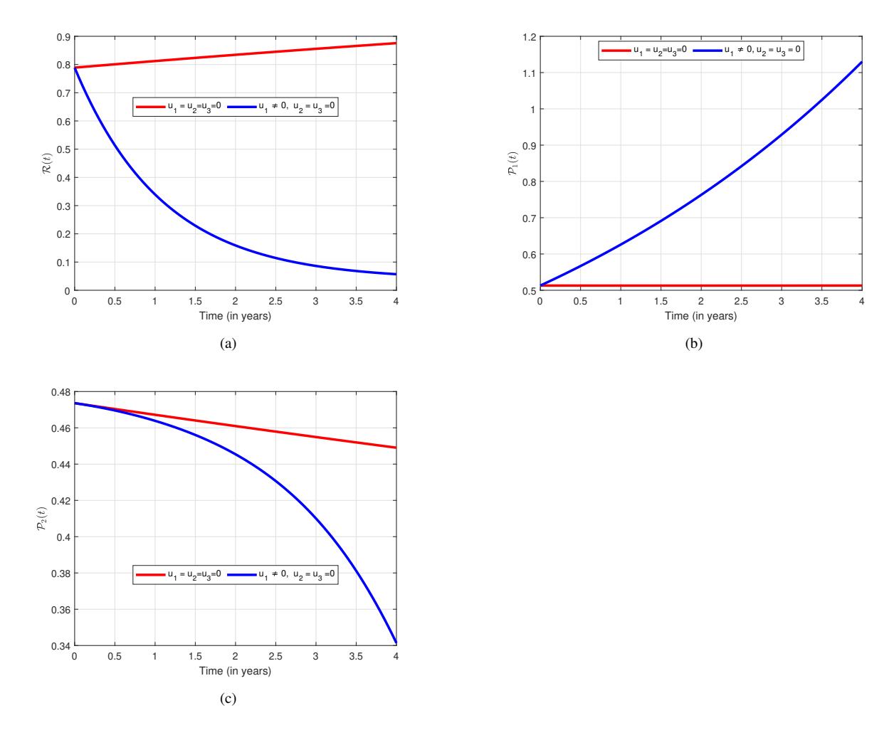
Figure 2: Simulation of the model with and without the optimal control \(u_1\).
5.2. Using Strategy 2: Implementing the persuasion effort \((u_2)\) of the party \(\mathcal{P}_2\)
This strategy focuses on registered voters who are undecided or willing to change their support for the party \(\mathcal{P}_2\). Given the variables \(u_1 = 0\), \(u_2 \neq 0\), and \(u_3 = 0\), the campaign will prioritize persuading efforts to convince registered voters to support the party \(\mathcal{P}_2\). This can be done by analyzing demographics, voting history, and interests based on issues to create targeted messaging. The results of the numerical situation are shown in Figure 3 with or without the control.
5.3. Using Strategy 3: The implementation effort of the electoral campaign \((u_3)\) by the electoral commission
This strategy focuses on persuading registered voters who are not interested in participating in the electoral process (U) to support a particular political party. Given the variables \(u_1 = 0\), \(u_2 = 0\), and \(u_3 \neq 0\), the campaign will prioritize efforts to engage these disconnected voters to understand their reasons for not being interested in voting. This can be achieved by analyzing demographics, voting history, and interests based on issues to understand the reasons for their disengagement. The results of the numerical situation are shown in Figure 4 with or without the control.
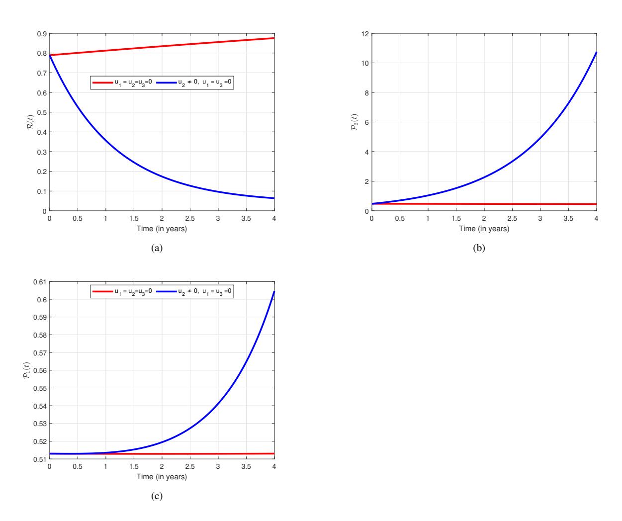
Figure 3: Simulation of the model with and without the optimal control \(u_2\).
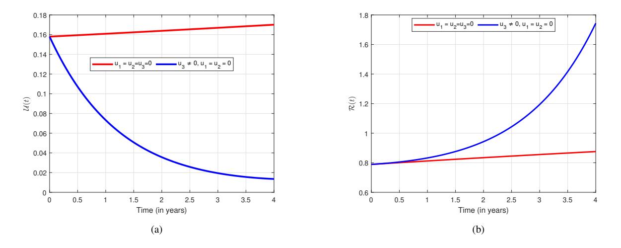
Figure 4: Simulation of the model with and without the optimal control \(u_3\).
5.4. Using Strategy 4: Implementing two controls
In this strategy, we combine the awareness campaign effort \((u_1)\) by the party \(\mathcal{P}_1\) and the persuasion effort \((u_2)\) by party \(\mathcal{P}_2\) \((u_1 \neq 0, u_2 \neq 0, u_3 = 0)\) to observe the effect on the voting class. We also combine the awareness campaign effort \((u_1)\) by the party \(\mathcal{P}_1\) and the campaign effort \((u_3)\) by the electoral commission \((u_1 \neq 0, u_2 = 0, u_3 \neq 0)\) to see the effect on the voting class. The results of the numerical situation are shown in Figure 5
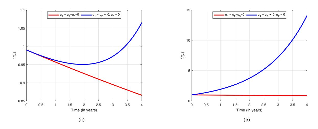
Figure 5: Simulation of the model with and without the optimal control \(u_1\) and \(u_2\).
5.5. Using Strategy 5: Implement all controls
In this strategy, we combine all the controls that is, the awareness campaign effort \((u_1)\) by the party \(\mathcal{P}_1\), the persuasion effort \((u_2)\) by party \(\mathcal{P}_2\) and the campaign effort by the electoral campaign \((u_3)\) of the electoral commission \((u_1 \neq 0, u_2 \neq 0, u_3 \neq 0)\) to see the effect on the registered voters and voting class.
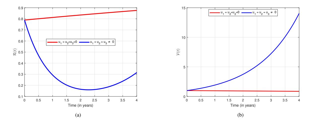
Figure 6: Simulation of the model with and without the optimal control \(u_1\), \(u_2\), and \(u_3\).
Initially, we examine the optimal control strategy \(u_1\) employed by the political party \(\mathcal{P}_1\). We notice that the number of registered voters who do not join any political party increases without the control, as shown in figure (2a), and the number of registered voters who join the political party \(\mathcal{P}_1\) decreases without the control, as seen in figure (2b). After applying the optimal control \(u_1\), we observe that the number of registered voters decreases, while those who join the political party \(\mathcal{P}_1\) gradually increase. The political party \(\mathcal{P}_2\) further decreases when control is applied.
Moreover, according to optimal control, \(u_2\) is chosen by the political party \(\mathcal{P}_2\). We observed that the number of registered voters who do not join any political party increases while the political party \(\mathcal{P}_2\) decreases without control, as shown in Figures (3a and 3b). The number of registered voters decreases when control is applied. The number of registered voters who have joined the political party \(\mathcal{P}_2\) has increased. In addition, we noticed that the registered voters who joined the political party \(\mathcal{P}_1\) gradually increased.
In addition, we consider the control \(u_3\). According to our analysis, without intervention, the current political climate would lead to a surge in registered voters who are not interested in voting, resulting in a significant drop in overall registered voters. However, after introducing optimal control \(u_3\), we observe a notable decrease in registered voters who did not have interest in voting \(\mathcal{U}\), accompanied by an increase in registered voters, as seen in Figures (4a and 4b). This suggests that \(u_3\) plays a crucial role in increasing voter engagement and registration.
In Figure (5), we combine the optimal controls \(u_1^*\) and \(u_2^*\) and set \(u_3=0\). In this strategy, the two optimal controls \(u_1^*\) and \(u_2^*\) are activated at the same time to improve the numerical results of Figure (5a). Control \(u_1(t)\) represents the effort of the awareness campaign to motivate registered voters to join \(\mathcal{P}_1\) and vote during the election, and control \(u_2(t)\) measures the required persuasion effort to change the position of registered voters in favor of a political party \(\mathcal{P}_2\). The rate of the voting class \(\mathcal{V}\) has experienced an increasing rate during four years. On the other hand, we combine the control \(u_1(t)\) representing the effort of the awareness campaign to motivate registered voters to join \(\mathcal{P}_1\) and vote during the election and the effort \(u_3(t)\) of the electoral campaign to impress registered voters who are not interested in participating in the electoral process and to support a political party by joining and voting. We notice that there is an increase in the voting class as shown in Figures (5a) and (5b). This indicates an increase in the participation rate in electoral processes.
Lastly, in Figure (6), we combine the optimal controls \(u_1^*\), \(u_2^*\), and \(u_3^*\) so that they are not zero. In this strategy, the three optimal controls \(u_1^*\), \(u_2^*\), and \(u_3^*\) are activated at the same time to improve the numerical results of Figure (6). \(u_3(t)\) represents the effort of the electoral campaign to impress registered voters who are not interested in participating in the electoral process and to support a political party by joining and voting. Figure (6a) shows that the proportion of registered voters \(\mathcal{R}\) has decreased after the introduction of controls, and the rate of registered voters moving to cast their vote has increased in Figure (6b). Interestingly, our analysis reveals that without control, the number of registered voters surged, as illustrated in the figure (6a). However, this increase was accompanied by a concerning decline in voting class participation. After applying the control, we observe that the number of registered voters decreases, which led to an increase in the voting class, as shown in Figure (6b). The number of voters who cast their vote decreases without control. After applying the controls, we notice that the number of voters who cast their vote has increased, as indicated in Figure (6b). This will help improve the participation rate during the election. This signifies that the control measures are effective.
6. CONCLUSION
In this article, we propose a fractional optimal control strategy for an awareness program that can help political parties increase the number of registered voters who join their party and vote during elections. The numerical results to support the analytical solutions have been extensively discussed. The model is validated using empirical data from the 2020 Ghana presidential elections. Our strategy incorporates three key controls to achieve this goal. The first control represents the awareness campaign effort (time, money, and human resources) to motivate registered voters to join \(\mathcal{P}_1\) and vote during an election. The second control measures the effort required persuasion effort to change the position of registered voters in favor of a political party \(\mathcal{P}_2\). The third control represents the effort of the electoral campaign to impress registered voters who are not interested in participating in the electoral process and to support a political party by joining and voting. Our findings indicate that implementing all three control measures is crucial to increasing voter participation in elections. This multifaceted approach will not only increase the participation rate but will also have a significant political impact. In addition, this will help reduce the number of registered voters who do not
cast their ballots, making the elections more representative and inclusive. By focusing on these three control areas, we can address the underlying issues that lead to low voter turnout. We recommend that registered voters be educated on the importance of participation and the impact of governance on their lives, and also encourage eligible citizens to register and vote.
ACKNOWLEDGEMENT
There was no funding for this research.
AVAILABILITY OF DATA
The data used can be found at the sites https://census2021.statsghana.go v.gh/gssmain/, https://ec.gov.gh/