

1. Introduction
In 1907, radiologist Ludwig Halberstadter and pathologist Stanislaus von Prowazek had discovered Chlamydia [1], [2], a sexually transmitted infection (STI) caused by a bacterium known as Chlamydia trachomatis (CT) [3]. In 2017, England recorded more than 203,116 new infections, compared to 44,676 for gonorrhea and 7,137 for syphilis [4]. The national screening program of Chlamydia concluded more than 126,000 Chlamydia cases among those aged 15 to 24. Although 80% of infected women remain asymptomatic, they can experience episodes of infertility due to blockage of the fallopian tubes [5]. In 1970s, Chlamydia was first known as a specific sexually transmitted disease (STD), but it remained unreported till 1988 [5]. Since 1990, cases have been reported regularly in sexually transmitted infection statistics, with a total of 34,000 new cases reported. After 1995, this number started to increase significantly, hitting 100,000 in 2003. In 2020, there were 128.5 million cases reported globally [6]. The sharp increase seemed to be genuine due to a rise in the number of sexual partners pursuing fertility treatment, and that youngsters have a high number of sexual companions. Demand for fertility services such as vitro fertilization and infertility treatment [7] has increased. With better sensitivity and particular diagnostic criteria, many cases of Chlamydia have been detected.
STDs, STIs, or sometimes called venereal diseases normally spread by direct contact with bodily fluids or genitals [8], [9]. CT is a bacterium that causes Chlamydia infection by spreading through vaginal, anal or oral
*Corresponding Author
Received August \(4^{th}\), 2025, Revised September \(10^{th}\), 2025, Accepted for publication September \(30^{th}\), 2025. Copyright ©2025 Published by Indonesian Biomathematical Society, e-ISSN: 2549-2896, DOI:10.5614/cbms.2025.8.2.1
sex. Chlamydia refers to a limited category of immotile coccoid bacteria [10] that are driven in eukaryotic cells to become intracellular parasites. Once the bacteria has entered a host, the mucous membrane of cells is affected by the bacteria. These are wet and soft tissues that are not covered by the skin of the human body such as the vagina, rectum, endometrium, the surfaces of the urethra, cervix, anus, eyelid membranes, abnormalities in the throat and fallopian tubes [11]. Commonly, the infection occurs in the endocervix of the woman. This infection is currently happening to almost 5 percent of women. Chlamydia can be transferred from an infected mother to her child [12] during vaginal birth, and it can result in pneumonia or neonatal eye infections for the latter [13]. These days, Chlamydia is becoming a common STD in men especially those who are young and sexually active. Almost 20 percent of men who have herpes are playing a major role to spread Chlamydia. Due to insufficiency of several metabolic paths, the cells of Chlamydia are not able to accomplish energy metabolism. As a result, they are completely dependent on a host cell that can provide them with Adenosine Triphosphate (ATP) or another antibody for energy [14]. Due to its dependency on the bio-synthetic machinery of the host, Chlamydia was initially misidentified as a virus. However, upon extensive studies, chlamydia is found to have a cell wall, deoxyribonucleic acid (DNA) that carries genetic information, ribosomes that are responsible for protein synthesis, and ribonucleic acid (RNA) which involves in coding, decoding, regulation and expression of DNA. Hence, it is classified as a bacterium. There are two variations of Chlamydia species that can cause STDs in humans namely CT and Chlamydia pneumoniae (also called the TWAR organism) while the other variation, Chlamydia psittaci, infects a wide range of mammals and birds[15], [16], [17].
More than 95 percent of infected people will recover if they take antibiotics properly. However, some of the STIs remain resistant to antibiotics, making the infections complicated and difficult to cure [18]. The easiest way to fight against Chlamydia is by preventing the spread from person to person. Infected people are to refrain from any sexual activity with all sexual partners until the infection is cleared. It is common for people to have multiple STDs, and it is crucial to receive therapy that is appropriate for each infection. For such diseases, precautionary measurements and antibiotic prescription are the basic treatment plan. There are some home-made remedies that are beneficial to reduce the symptoms Echinacea plant can increase immunity level and help to fight against various bacterial and viral infections [19]. However, since this plant can only manage the symptoms, it has to be used together with the prescribed antibiotics. Goldenseal plant can also be used to reduce STIs such as gonorrhea and Chlamydia. Olive leaf extract or olive tree extract is another candidate known to reduce pain and inflammation. However, more research on the effectiveness of these plants in treating STDs are needed. Chlamydia infection requires extensive care and effort since it has complicated, severe health impacts as well as dangerous social implications.
To understand the mechanism of the disease's like chlamydia spread at the community level, several scholars have examined the illness using mathematical models [20], [21], [22]. Wilson [23] demonstrated a disease Chlamydia infection model that represents the scatters of infection inside human cells. Additionally, the cause of developmental cycle of the Chlamydia and the hypotheses on the pathophysiology of the disease based on the model were discussed. Adetunde et al. [24] evaluated the effect of CT bacterial infections in people. Mushayabasa [25] conducted a thorough analysis of a deterministic model and evaluated the epidemiological effects of co-infection of gonorrhea and Chlamydia. Sharomi and Gumel [26], [27], [28] described the changing patterns of CT transmission. Recently, Samanta and Sharma [29] performed an analysis of a model of a delayed Chlamydia outbreak using pulse vaccination. There are many mathematical models established for this disease [30], [31], [32]. The canonical approach has been adopted to model the force of infection [33], [34]. More advanced models include vaccination and other infections [35], [36], [37], [38], [39]. In order to completely understand the behavior of the disease, solutions for the mathematical models should be generated. Numerical methods become crucial to generate them since exact solutions are complicated and almost impossible to calculate. Dynamical systems often demonstrate few necessary features like boundedness, positivity etc. Good numerical methods preserve these physical properties. To solve dynamical systems, different authors used various techniques [40], [41], [42]. Mathematical modelling by delay differential equations is essential in the field of epidemiology, particularly for tackling real-world challenges like viral diseases as well as by neural networking [43].
The primary objective of this research is to develop a novel Chlamydia epidemic model that incorporates exponential time delay, providing a more realistic representation of disease dynamics. To achieve this, we extend the Chlamydia epidemic model [44] by incorporating a exponential time delay. Unlike previous models, our approach explicitly accounts for delay-induced stability shifts, offering deeper insights into the long-term behavior of the epidemic. The model's theoretical properties, including equilibrium analysis, sensitivity analysis and stability conditions, are rigorously examined to ensure its reliability. The inclusion of time delay significantly influences the epidemic's progression, affecting both equilibrium states and longterm stability. Additionally, an efficient numerical approach is applied to examine the resulting nonlinear delay differential equation system. Numerical simulations are performed as a secondary step to illustrate the model's behavior and validate its theoretical predictions. In recent years, various numerical techniques have been employed to study infectious disease models, including Euler's method, RK4 methods, and finite difference schemes. However, these classical methods often fail to preserve essential qualitative features of the underlying biological system, such as positivity, boundedness, and dynamical consistency, especially when applied to models involving delay or nonlinearity. In contrast, the Nonstandard Finite Difference (NSFD) method, introduced by Mickens [46], has shown significant advantages in accurately capturing the longterm behavior of epidemic models [47]. The NSFD approach ensures that solutions remain non-negative and biologically meaningful, regardless of the chosen time step. This is particularly important in disease modeling, where negative population values are non-physical and can lead to misleading conclusions [48], [49], [50], [51]. Moreover, NSFD schemes can be adapted to preserve equilibrium points and their stability properties, which is often not guaranteed in standard methods [52], [53], [54]. In our study, the application of the NSFD method to a time-delay Chlamydia model not only improves numerical stability but also provides more reliable and realistic simulations that align with theoretical predictions. Compared to other established approaches, our method offers a robust and structure-preserving framework, making it especially suitable for modeling infectious diseases with delay dynamics. This superiority justifies the choice of NSFD for the current work and lays the groundwork for further extensions into fractional, stochastic, or spatio-temporal domains. Unlike classical methods such as Euler and RK4, the NSFD scheme satisfies generalized stability and convergence criteria for nonlinear problems, as discussed by Ciegis et al. [55]. This ensures numerical solutions remain stable and biologically consistent even with larger step sizes, making NSFD a more robust tool for modeling Chlamydia dynamics. To our knowledge, this is the first time such a delayed epidemiological model for Chlamydia has been analyzed in this specific form, particularly with its novel stability characterization and equilibrium assessment. Furthermore, to the best of our knowledge, this model has not been previously solved using the NSFD method.
The paper is arranged as follows: A literature review on infection with a concise background about and similar to Chlamydia is outlined in Section 1. The modification of an existing Chlamydia epidemics model is presented in Section 2; the equilibrium points, existence and uniqueness of model solution are explored in Section 3. The reproductive number and its parameter sensitivity are addressed in Section 4. The local and global stability of the system are discussed in Section 5. Investigation of the NSFD scheme's convergence along with the results of numerical simulations at different points are presented in Section 6. Lastly, this paper is concluded in Section 7.
2. DELAY MATHEMATICAL MODEL
Chlamydia disease impact may be further controlled if delay strategies are implemented on humans. For this purpose, we have incorporated \(\tau\) as exponential time delay rate factor that can reduce disease spread, and the negative sign with \(\mu\) indicates that our problem is an initial value problem, moving toward initial values when the delay term is applied. A model from [44] is selected and interventional measures between susceptible and infected humans are applied. The model formulation uses the following compartmental information
- S(t) represents the susceptible community.
- \(\bullet\) E(t) indicates the exposed community.
- \(I_A(t)\) describes the community in Asymptomatic phase.
- \(I_S(t)\) describes the individuals in Symptomatic phase.
- R(t) represents the number of recovered individuals.
The host population of size N(t) consists of susceptible S(t), exposed E(t), asymptomatic \(I_A(t)\), symptomatic humans \(I_S(t)\), as well as individuals who have recovered R(t), defined as
Population (N) = Susceptible + Exposed + Asymptomatic + Symptomatic + Recovered \[(1)\]
Let \(\Lambda\) represent the rate at which new individuals join the susceptible category, influenced by factors such as recruitment or the birth rate of the susceptible population. The transmission of the disease occurs when individuals move from the susceptible group to infected asymptomatic group through direct connection with the infectious community with the rate of β1. Similarly, transmission from the susceptible compartment to the infected symptomatic compartment happens at a rate of β2 due to direct interaction with infectious persons. The parameter µ represents the intrinsic mortality rate of the susceptible community. Additionally, α denotes the proportion of the recovering class that remains susceptible to reinfection. Hence, the total variation in the number of susceptible hosts is described using the differential equation below
\[\frac{dS}{dt} = \Lambda - \beta_1 S I_A e^{-\mu\tau} - \beta_2 S I_S e^{-\mu\tau} - \mu S + \alpha R.\]
In the exposed class, τ represents the time delayed to the direct transfer of the infection in both the asymptomatic and symptomatic compartments, and the negative sign with µ indicates that our problem is an initial value problem, approaching toward initial values when the delay term is applied. The terms ρη is the ratio of the individuals who do not have the symptoms of Chlamydia infection but still can infect other individuals and transfer to the group IA. µ represents the natural death rates, affecting the exposed community. The change in the exposed population E(t) over time is described by the differential equation (DE)
\[\frac{dE}{dt} = \beta_1 S I_A e^{-\mu \tau} + \beta_2 S I_S e^{-\mu \tau} - \rho \eta E - \mu E.\]
The individuals infected from infection but without symptoms belong to the compartment IA. The terms ρη is the remaining fraction of the individual who does not show symptoms of Chlamydia infection but still have ability to infect others and transfer to the community IA. The rate of recovery in this compartment is denoted by kr1, after these individuals move to the class R. So, the DE for the system at change in infected community in asymptomatic phase IA is
\[\frac{dI_A}{dt} = \rho \eta E - (r_1 + \mu)I_A.\]
The individuals infected from infection showing symptoms of infection, enter to the compartment IS. (1−ρ)η is the newly infected individual's fraction who will start to adopt symptoms of Chlamydia disease and transmit to the group IS. The rate at which the asymptomatically infectious individuals eventually show disease symptoms transfer to the group IS is represented by (1−κ)r1. The death rate in this compartment is denoted by µ, r2 is the rate at which the infectious individuals showing symptoms of Chlamydia (in symptomatic phase) clear infections and migrate to the class R. Thus, for the rate of change of infected individuals in symptomatic phase IS, the model differential equation is
\[\frac{dI_S}{dt} = (1 - \rho)\eta E + (1 - \kappa)r_1 I_A - (r_2 + \mu)I_S.\]
The individuals recovered from infection transfer to the class R. The ratio at which infected individual in asymptomatic phase not showing symptoms of Chlamydia infection, recovered is κr1. r2 represents the proportion of infectious individuals in the symptomatic phase of Chlamydia who recover and transition to class R, while the intrinsic death rate µ impacts the recovered individuals. The ratio of recovered class that become susceptible again is α. Therefore, the DE representing this mechanism in recovered community is
\[\frac{dR}{dt} = \kappa r_1 I_A + r_2 I_S - \mu R - \alpha R.\]
Numerical and graphical analyses for this model were conducted using the parametric dimensions shown in Table 1.
Figure 1 displays the extended, proposed chlamydia model after adding the exponential delay factor. The
| Parameters | DFP / EEP | Reference |
|---|---|---|
| Λ | 1.12 | [44] |
| \(\beta_1\) | 0.1 | [44] |
| \(\beta_2\) | 0.15 | [44] |
| \(\mu\) | 0.15 | [44] |
| \(\alpha\) | 0.5 | [44] |
| \(\eta\) | 0.5 | [44] |
| \(\rho\) | 0.7 | [44] |
| \(r_1\) | 0.7 | [44] |
| \(r_2\) | 0.8 | [44] |
| \(\kappa\) | 0.7 | [44] |
| \(\tau\) | \(\geq 0\) | Assumed |
Table 1: Parametric values used in this study.
Figure 1: Chlamydia delay model.
accompanying system of delay differential equations is as follows
\[\frac{dS}{dt} = \Lambda - \beta_1 S I_A e^{-\mu \tau} - \beta_2 S I_S e^{-\mu \tau} - \mu S + \alpha R, \tag{2a}\]
\[\frac{dS}{dt} = \Lambda - \beta_1 S I_A e^{-\mu\tau} - \beta_2 S I_S e^{-\mu\tau} - \mu S + \alpha R, \qquad (2a)\] \[\frac{dE}{dt} = \beta_1 S I_A e^{-\mu\tau} + \beta_2 S I_S e^{-\mu\tau} - \rho \eta E - \mu E, \qquad (2b)\] \[\frac{dI_A}{dt} = \rho \eta E - (r_1 + \mu) I_A, \qquad (2c)\] \[\frac{dI_S}{dt} = (1 - \rho) \eta E + (1 - \kappa) r_1 I_A - (r_2 + \mu) I_S, \qquad (2d)\] \[\frac{dR}{dt} = \kappa r_1 I_A + r_2 I_S - \mu R - \alpha R, \qquad (2e)\]
\[\frac{dI_A}{dt} = \rho \eta E - (r_1 + \mu)I_A,\tag{2c}\]
\[\frac{dI_S}{dt} = (1 - \rho)\eta E + (1 - \kappa)r_1 I_A - (r_2 + \mu)I_S,\] (2d)
\[\frac{dR}{dt} = \kappa r_1 I_A + r_2 I_S - \mu R - \alpha R,\tag{2e}\]
with starting points
\[S(0) > 0\], \(E(0) \ge 0\), \(I_A(0) \ge 0\), \(I_S(0) \ge 0\), \(R(0) \ge 0\). (2f)
Here \(t \ge 0\), \(\tau \le t\).
3. MODEL ANALYSIS
In this segment, a conceptual analysis of the dynamics exhibited by Chlamydia infection are calculated. This analysis consists of model properties, namely the positivity, boundedness of solution and model equilibrium states
Theorem 3.1. The proposed model 2 of disease possesses a non-negative solution for non-negative initial conditions for all \(t \ge 0\).
Proof: Consider the differential inequality for the susceptible population S:
\[\frac{dS}{S} \ge -\left(\beta_1 I_A e^{-\mu\tau} + \beta_2 I_S e^{-\mu\tau} + \mu\right).\]
To show that \(S(t) \ge 0\) for all \(t \ge 0\), given that \(S(0) = S_0 \ge 0\), both sides are integrated with respect to t over the interval \([t, t_0]\):
\[\int_{t}^{t_0} \frac{dS}{S} dt \ge - \int_{t}^{t_0} \left( \beta_1 I_A e^{-\mu \tau} + \beta_2 I_S e^{-\mu \tau} + \mu \right) dt.\]
Evaluating the integral on the left side yield
\[\ln \frac{S(t_0)}{S(t)} \ge -\left(\beta_1 e^{-\mu\tau} \int_t^{t_0} I_A(t) dt + \beta_2 e^{-\mu\tau} \int_t^{t_0} I_S(t) dt + \mu(t_0 - t)\right).\]
Substituting \(t = t_0\) and \(S(t_0) = S_0\) leads to
\[\ln \frac{S_0}{S(t)} \ge -\left(\beta_1 e^{-\mu\tau} \int_t^{t_0} I_A(t) dt + \beta_2 e^{-\mu\tau} \int_t^{t_0} I_S(t) dt + \mu(t_0 - t)\right).\]
Since the integrals over a zero-length interval are zero,
\[\int_{t}^{t_0} I_A(t) dt = 0, \quad \int_{t}^{t_0} I_S(t) dt = 0,\] and \((t_0 - t) = 0\), the inequality simplifies to
\[\ln \frac{S_0}{S(t)} \ge 0.\]
Exponentiating both sides yields
\[\frac{S_0}{S(t)} \ge 1.\]
Thus,
\[S_0 > S(t)\].
\(S_0 \ge 0\) from the initial condition and \(S(t) \le S_0\). As a result, \(S(t) \ge 0\) for all \(t \ge 0\). Therefore, the model's solution S(t) is non-negative for all \(t \ge 0\), provided that the initial condition \(S(0) = S_0 \ge 0\). Also, we can analyze positivity as
\[\begin{aligned} \frac{dS}{dt}\bigg|_{S=0} &= \Lambda + \alpha R \geq 0, & \frac{dE}{dt}\bigg|_{E=0} &= \beta_1 S I_A e^{-\mu\tau} + \beta_2 S I_S e^{-\mu\tau} \geq 0, \\ \frac{dI_A}{dt}\bigg|_{I_A=0} &= \rho \eta E \geq 0, & \frac{dI_S}{dt}\bigg|_{I_S=0} &= (1-\rho)\eta E + (1-\kappa)r_1 I_A \geq 0, \\ \frac{dR}{dt}\bigg|_{R=0} &= \kappa r_1 I_A + r_2 I_S \geq 0, & \end{aligned}\] which indicates that the system maintains positivity under the given initial conditions (2f).
Theorem 3.2. Solutions of the proposed system are all bounded in feasible region \(\Omega\).
Proof: Let the total population \(N(t) = S(t) + E(t) + I_A(t) + I_S(t) + R(t)\). Summing the differential equations yields
\[\frac{dN}{dt} = \dot{S} + \dot{E} + \dot{I}_A + \dot{I}_S + \dot{R}.\]
Substituting the right-hand sides of the equations, we get
\[\frac{dN}{dt} = \Lambda - \mu(S + E + I_A + I_S + R).\]
Upon simplifying the equation, we obtain the following linear differential equation
\[\frac{dN}{dt} = \Lambda - \mu N(t).\]
In order to solve it, the variables are separated and integrated to become
\[\int \frac{dN}{\Lambda - \mu N} = \int dt.\]
Integrating both sides, we obtain
\[-\frac{1}{\mu}\ln\left(\Lambda - \mu N\right) = t + C.\]
Exponentiating both sides gives
\[\Lambda - \mu N = Ce^{-\mu t}.\]
Solving for N(t), we find
\[N(t) = \frac{\Lambda}{\mu} + \left(N(0) - \frac{\Lambda}{\mu}\right) e^{-\mu t}.\]
As \(t \to \infty\), the exponential term \(e^{-\mu t} \to 0\), implying:
\[N(t) \to \frac{\Lambda}{\mu}\].
Thus, \(N(t) \leq \frac{\Lambda}{\mu}\) for all \(t \geq 0\). Therefore, the whole population N(t) is bounded and satisfies \(0 < N(t) \leq \frac{\Lambda}{\mu}\). This ensures that all solutions remain within efficient region \(\Omega\)
\[\Omega = \left\{ (S(t), E(t), I_A(t), I_S(t), R(t)) \in \mathbb{R}_+^5 \mid 0 < N(t) \le \frac{\Lambda}{\mu} \right\}.\] (3)
3.1. Model Equilibrium Points
The system will be illustrated with two different forms of equilibrium, indicated by \(\varepsilon_0\) and \(\varepsilon_1\), which represent disease-free (DF) and endemic equilibrium (EE) points, respectively.
\[\varepsilon_0 = (S_0, E_0, I_{A_0}, I_{S_0}, R_0) = (\frac{\Lambda}{\mu}, 0, 0, 0, 0),\]
\[\varepsilon_1 = (S_1, E_1, I_{A_1}, I_{S_1}, R_1) = (S^*, E^*, I_A^*, I_S^*, R^*),\] with coordinates,
\[E^* = \frac{(r_1 + \mu)I_A^*}{\rho\eta}, \quad I_S^* = \frac{[(1 - \rho)(r_1 + \mu) + \rho(1 - \kappa)r_1]I_A^*}{(r_2 + \mu)\rho},\] \[R^* = \frac{[\kappa r_1(r_2 + \mu)\rho + r_2((1 - \rho)(r_1 + \mu) + (1 - \kappa)\rho r_1)]I_A^*}{(\mu + \alpha)(r_2 + \mu)\rho},\] \[S^* = \frac{(r_1 + \mu)(r_2 + \mu)(\rho\eta + \mu)}{\eta e^{-\mu\tau}[\beta_1\rho(r_2 + \mu) + \beta_2((1 - \rho)(r_1 + \mu) + \rho(1 - \kappa)r_1)]},\] \[I_A^* = \frac{\Lambda(1 - \frac{1}{\mathcal{R}_0})\rho\eta(r_2 + \mu)(\mu + \alpha)}{\sigma}.\]
Here \(\mathcal{R}_0 > 0\) and, \(\mathbf{g} = (\frac{\Lambda}{\mu} \frac{1}{R_0} \beta_1 (1 - e^{-\mu \tau}) \rho \eta(r_2 + \mu) (\mu + \alpha) + \beta_2 \frac{\Lambda}{\mu} \frac{1}{R_0} \eta(\mu + \alpha) [r_1 + \mu(1 - \rho) - \rho \kappa r_1] (1 - e^{-\mu \tau}) + [-\alpha \eta(\rho r_1 (1 - \kappa + \mu \kappa)) + r_2 (r_1 (1 + \rho \kappa - \rho) + \mu(1 - \rho))] + (r_2 + \mu) (\mu + \alpha) (\rho \eta + \mu) (r_1 + \mu)).\)
3.2. Existence and Uniqueness
This section represents the uniqueness and existence of the model's solutions using the Banach's fixed point theorem. The first step is to demonstrate that the solution
\[(S, E, I_A, I_S, R),\]
along with the initial conditions (2f), are both bounded and non-negative for all \(t \ge 0\). Given that all model parameters are positive, we can consider the following equations
\[\frac{dS}{dt} \ge -\left(\beta_1 I_A e^{-\mu\tau} + \beta_2 I_S e^{-\mu\tau} + \mu\right) S\] \[\Rightarrow \frac{dS}{S} \ge -\left(\beta_1 I_A e^{-\mu\tau} + \beta_2 I_S e^{-\mu\tau} + \mu\right) dt.\] \[\frac{dE}{dt} \ge -\left(\rho\eta + \mu\right) E \Rightarrow \frac{dE}{E} \ge -\left(\rho\eta + \mu\right) dt.\] \[\frac{dI_A}{dt} \ge -\left(r_1 + \mu\right) I_A \Rightarrow \frac{dI_A}{I_A} \ge -\left(r_1 + \mu\right) dt.\] \[\frac{dI_S}{dt} \ge -\left(r_2 + \mu\right) I_S \Rightarrow \frac{dI_S}{I_S} \ge -\left(r_2 + \mu\right) dt.\] \[\frac{dR}{dt} \ge -\left(\mu + \alpha\right) R \Rightarrow \frac{dR}{R} \ge -\left(\mu + \alpha\right) dt.\] (4)
Equation (4) is then solved, with initial conditions
\[S(t) = S(0)e^{-\int_0^t (\beta_1 I_A(t)e^{-\mu\tau} + \beta_2 I_S(t)e^{-\mu\tau} + \mu)dt} \ge 0.\] \[E(t) = E(0)e^{-\int_0^t (\rho\eta + \mu)dt} \ge 0.\] \[I_A(t) = I_A(0)e^{-\int_0^t (r_1 + \mu)dt} \ge 0.\] \[I_S(t) = I_{S1}(0)e^{-\int_0^t (r_2 + \mu)dt} \ge 0.\] \[R(t) = R(0)e^{-\int_0^t (\mu + \alpha)dt} \ge 0.\] (5)
As a result, the model's solutions, including the initial conditions, remain non-negative for all \(t \ge 0\). Since \(N = S + E + I_A + I_S + R\), thus all functions within the system are bounded
\[0 \le S(t) \le N, \quad 0 \le E(t) \le N, \quad 0 \le I_A(t) \le N, 0 < I_{S1}(t) < N, \quad 0 < R(t) < N.\] (6)
At this point, theorems concerning the existence and uniqueness of solutions can be presented. Let's consider the starting conditions for the system as follows
\[(S(0), E(0), I_A(0), I_S(0), R(0)) = (S_0, E_0, I_{\Lambda_0}, I_{S_0}, R_0). \tag{7}\]
Applying the integral operator \(\int_0^t (\cdot) dt\) to the model results in
\[S(t) - S(0) = \int_{0}^{t} (\Lambda - \beta_{1} S I_{A} e^{-\mu \tau} - \beta_{2} S I_{S} e^{-\mu \tau} - \mu S + \alpha R) dt,\] \[E(t) - E(0) = \int_{0}^{t} (\beta_{1} S I_{A} e^{-\mu \tau} + \beta_{2} S I_{S} e^{-\mu \tau} - \rho \eta E - \mu E) dt,\] \[I_{A}(t) - I_{A}(0) = \int_{0}^{t} (\rho \eta E - r_{1} I_{A} - \mu I_{A}) dt,\] \[I_{S}(t) - I_{S}(0) = \int_{0}^{t} ((1 - \rho) \eta E + (1 - \kappa) r_{1} I_{A} - (r_{2} + \mu) I_{S}) dt,\] \[R(t) - R(0) = \int_{0}^{t} (\kappa r_{1} I_{A} + r_{2} I_{S} - \mu R - \alpha R) dt.\] (8)
The final equation's solution is formulated by assuming that \(N = S + E + I_A + I_S + R\). For the sake of clarity, the following kernels are established
\[\mathcal{K}_{1}(t,S) = \Lambda - \beta_{1} S I_{A} e^{-\mu\tau} - \beta_{2} S I_{S} e^{-\mu\tau} - \mu S + \alpha R, \mathcal{K}_{2}(t,E) = \beta_{1} S I_{A} e^{-\mu\tau} + \beta_{2} S I_{S} e^{-\mu\tau} - \rho \eta E - \mu E, \mathcal{K}_{3}(t,I_{A}) = \rho \eta E - (r_{1} + \mu) I_{A}, \mathcal{K}_{4}(t,I_{S}) = (1-\rho) \eta E + (1-\kappa) r_{1} I_{A} - (r_{2} + \mu) I_{S}, \mathcal{K}_{5}(t,R) = \kappa r_{1} I_{A} + r_{2} I_{S} - \mu R - \alpha R.\] (9)
Since \(S, E, I_A, I_S, R\) are non-negative bounded functions, it follows that there exist positive values \(\sigma_i, i = 1, 2, \dots, 5\) as a result
\[||S(t)|| \le \sigma_1, \quad ||E(t)|| \le \sigma_2, \quad ||I_A(t)|| \le \sigma_3,\]
\(||I_S(t)|| \le \sigma_4, \quad ||R(t)|| \le \sigma_5.\) (10)
So, Equation (8) can be written as
\[S(t) - S(0) = \int_0^t \mathcal{K}_1(\tau, S(\tau)) d\tau, \qquad E(t) - E(0) = \int_0^t \mathcal{K}_2(\tau, E(\tau)) d\tau,\] \[I_A(t) - I_A(0) = \int_0^t \mathcal{K}_3(\tau, I_A(\tau)) d\tau, \qquad I_S(t) - I_S(0) = \int_0^t \mathcal{K}_4(\tau, I_S(\tau)) d\tau,\] \[R(t) - R(0) = \int_0^t \mathcal{K}_5(\tau, R(\tau)) d\tau.\] (11)
Theorem 3.3. If \(0 \le \Gamma = \max_{1 \le i \le 5} \{\gamma_i\} < 1\), then the kernels \(K_i\) for \(1 \le i \le 5\) fulfill the Lipschitz condition and qualify as contraction mappings.
Proof: Let us consider kernel \(K_1\). Suppose that S(t) and \(S_1(t)\) be two respectively arbitrary functions, then one possesses
\[\| \mathcal{K}_{1}(t,S) - \mathcal{K}_{1}(t,S_{1}) \| \leq \| \Lambda - \beta_{1} S I_{A} e^{-\mu\tau} - \beta_{2} S I_{S} e^{-\mu\tau} - \mu S + \alpha R\] \[-\Lambda + \beta_{1} S_{1} I_{A} e^{-\mu\tau} + \beta_{2} S_{1} I_{S} e^{-\mu\tau} + \mu S_{1} - \alpha R \|\] \[\leq \beta_{1} I_{A} \| S - S_{1} \| + \beta_{2} I_{S} \| S - S_{1} \|\] \[+ \mu \| S - S_{1} \|\] \[= g_{1} \| S - S_{1} \|.\] (12)
Similar procedure is applied to obtain
1) Kernel K2
\[\| \mathcal{K}_{2}(t,E) - \mathcal{K}_{2}(t,E_{1}) \| \leq \| \beta_{1} S I_{A} e^{-\mu\tau} + \beta_{2} S I_{S} e^{-\mu\tau} - \rho \eta E - \mu E\] \[-\beta_{1} S I_{A} e^{\Lambda_{\tau}} - \beta_{2} S I_{S} e^{-\mu\tau} + \rho \eta E_{1} + \mu E_{1} \|\] \[\leq \rho \eta \| E - E_{1} \| + \mu \| E - E_{1} \|\] \[= g_{2} \| E - E_{1} \|.\] (13)
2) Kernel K3
\[\| \mathcal{K}_{3}(t, I_{A}) - \mathcal{K}_{3}(t, I_{\Lambda 1}) \| \leq \| \rho \eta E - (r_{1} + \mu) I_{A} - \rho \eta E + (r_{1} + \mu) I_{\Lambda 1}\] \[\leq (r_{1} + \mu) \| I_{A} - I_{\Lambda 1} \|\] \[= g_{3} \| I_{A} - I_{\Lambda 1} \| .\] (14)
3) Kernel K4
\[\| \mathcal{K}_{4} (t, I_{S}) - \mathcal{K}_{4} (t, I_{S1}) \| \leq \| (1 - \rho) \eta E + (1 - \kappa) r_{1} I_{A} - (r_{2} + \mu) I_{S} - (1 - \rho) \eta E + (1 - \kappa) r_{1} I_{A} - (r_{2} + \mu) I_{S1} \leq (r_{2} + \mu) \| I_{S} - I_{S1} \| = g_{4} \| I_{S} - I_{S1} \|.\] \[(15)\]
4) Kernel K5
\[\| \mathcal{K}_{5}(t,R) - \mathcal{K}_{5}(t,R_{1}) \| \leq \| \kappa r_{1} I_{A} + r_{2} I_{S} - \mu R - \alpha R - \kappa r_{1} I_{A} - r_{2} I_{S} + \mu R_{1} + \alpha R_{1}\] \[\leq \mu \| R - R_{1} \| + \alpha \| R - R_{1} \|\] \[= g_{5} \| R - R_{1} \|.\] (16)
Consequently, the Lipschitz criteria [45] are fulfilled for Ki , i = 1, 2, · · · , 5. As, 0 ≤ Γ < 1, the contradiction in mappings by kernels. So now, by using Equation (11), the formulas are rewritten as
\[S_{n}(t) = \int_{0}^{t} \mathcal{K}_{1}(\tau, S_{n-1}(\tau)) d\tau, \qquad E_{n}(t) = \int_{0}^{t} \mathcal{K}_{2}(\tau, E_{n-1}(\tau)) d\tau,\] \[I_{A_{n}}(t) = \int_{0}^{t} \mathcal{K}_{3}(\tau, I_{A_{n-1}}(\tau)) d\tau, \qquad I_{S_{n}}(t) = \int_{0}^{t} \mathcal{K}_{4}(\tau, I_{S_{n-1}}(\tau)) d\tau,\] \[R_{n}(t) = \int_{0}^{t} \mathcal{K}_{5}(\tau, R_{n-1}(\tau)) d\tau.\] (17)
In the recursive formulas, differences between two consecutive terms are as follows
\[\chi_{l} = S_{l} - S_{m} = \int_{0}^{t} \left( \mathcal{K}_{1} \left( \tau, S_{m}(\tau) \right) - \mathcal{K}_{1} \left( \tau, S_{p}(\tau) \right) \right) d\tau,\] \[\varphi_{l} = E_{l} - E_{m} = \int_{0}^{t} \left( \mathcal{K}_{2} \left( \tau, E_{m}(\tau) \right) - \mathcal{K}_{2} \left( \tau, E_{p}(\tau) \right) \right) d\tau,\] \[\psi_{l} = I_{A_{l}} - I_{A_{m}} = \int_{0}^{t} \left( \mathcal{K}_{3} \left( \tau, I_{A_{m}}(\tau) \right) - \mathcal{K}_{3} \left( \tau, I_{A_{p}}(\tau) \right) \right) d\tau,\] \[\eta_{l} = I_{S_{l}} - I_{S_{m}} = \int_{0}^{t} \left( \mathcal{K}_{4} \left( \tau, I_{S_{m}}(\tau) \right) - \mathcal{K}_{4} \left( \tau, I_{S_{p}}(\tau) \right) \right) d\tau,\] \[\zeta_{l} = R_{l} - R_{m} = \int_{0}^{t} \left( \mathcal{K}_{5} \left( \tau, R_{m}(\tau) \right) - \mathcal{K}_{5} \left( \tau, R_{p}(\tau) \right) \right) d\tau.\] (18)
Where, l=n, m=n-1 and p=n-2. So, one can conclude that
\[S_{l}(t) = \sum_{i=1}^{l} \chi_{l}(t), \qquad E_{l}(t) = \sum_{i=1}^{l} \varphi_{l}(t), \qquad I_{A_{l}}(t) = \sum_{i=1}^{l} \psi_{l}(t),\] \[I_{S_{l}}(t) = \sum_{i=1}^{l} \eta_{l}(t), \qquad R_{l}(t) = \sum_{i=1}^{l} \zeta_{l}(t).\] (19)
Recursive inequalities for the differences in Equation (18) are calculated as follows
\[\|\chi_{l}\| = \|S_{l} - S_{m}\|\] \[= \left\| \int_{0}^{t} \left( \mathcal{K}_{1} \left( \tau, S_{m}(\tau) \right) - \mathcal{K}_{1} \left( \tau, S_{p}(\tau) \right) \right) d\tau \right\|,\] \[\leq \int_{0}^{t} \| \left( \mathcal{K}_{1} \left( \tau, S_{m}(\tau) \right) - \mathcal{K}_{1} \left( \tau, S_{p}(\tau) \right) \right) d\tau \|,\] \[\leq \lambda_{1} t \| \left( S_{m}(t) - S_{p}(t) \right) \|,\] \[= \gamma_{1} t \| \chi_{l}(t) \|,\] \[\| \varphi_{l}(t) \| \leq \gamma_{2} t \| \varphi_{l}(t) \|, \quad \| \psi_{l}(t) \| \leq \lambda_{3} t \| \psi_{l}(t) \|,\] \[\| \eta_{l}(t) \| \leq \gamma_{4} t \| \eta_{l}(t) \|, \quad \| \zeta_{l}(t) \| \leq \gamma_{5} \| \zeta_{l}(t) \|.\] \[(20)\]
Theorem 3.4. If the following inequalities hold for a time \(T_0 > 0\): \(0 < \gamma_i T_0 < 1\) for i = 1, 2, ..., 5, then there exists a unique solution for the proposed model.
Proof: This section is divided into two parts, which are existence and uniqueness.
1) Existence. Every function within the model is bounded, and the given kernels fulfil the Lipschitz criteria. Consequently, by Equation (20) the following inequalities can be derived
\[\|\chi_{n}(t)\| \leq \lambda_{1}t \|\chi_{n-1}\| \leq (\gamma_{1}t)^{2} \|\chi_{n-2}(t)\| \leq \dots \leq \|S(0)\| (\gamma_{1}t)^{n},\]
\[\|\varphi_{n}(t)\| \leq \|E(0)\| (\gamma_{2}t)^{n}, \quad \|\psi_{n}(t)\| \leq \|I_{A}(0)\| (\gamma_{3}t)^{n},\]
\[\|\eta_{n}(t)\| \leq \|I_{S}(0)\| (\gamma_{4}t)^{n}, \quad \|\zeta_{n}(t)\| \leq \|R(0)\| (\gamma_{5}t)^{n}.\]
(21)
In accordance with Equation (21), the defined functions in Equation (19) exist and are smooth. We explain that, functions \(S_n(t)\), \(E_n(t)\), \(I_{\Lambda_n}(t)\), \(I_{S_n}(t)\), \(R_n(t)\) converge to solutions of system. We define \(A_n^i(t)\), \(i = 1, 2, \dots, 5\), as the remaining terms following n iterations, specifically
\[S(t) - S(0) = S_n(t) + A_n^1(t), E(t) - E(0) = E_n(t) + A_n^2(t),\] \[I_A(t) - I_A(0) = I_{\Lambda_n}(t) + A_n^3(t), I_S(t) - I_S(0) = I_{S_n}(t) + A_n^4(t),\] \[R(t) - R(0) = R_n(t) + A_n^5(t).\] (22)
By using the condition of Lipschitz for \(K_1\) leads to
\[||A_{n}^{1}|| = ||\int_{0}^{t} (\mathcal{K}_{1}(\tau, S) - \mathcal{K}_{1}(\tau, S_{n-1})) d\tau)|| \le \gamma_{1}t ||S - S_{n-1}||\] \[\le (\gamma_{1}t)^{2} ||S - S_{n-2}|| \le \cdots \le (\gamma_{1}t)^{2} ||A_{0}^{1}(t)||\] \[\le (\gamma_{1}t)^{n} ||S(t)|| \le (\gamma_{1}t)^{n} \varrho_{1}.\] (23)
By setting \(t = T_0\), one obtains
\[||A_n^1(t)|| \le (\gamma_1 T_0)^n \varrho_1. \tag{24}\]
Calculating the limit of inequality in Equation (24) as n approaches \(\infty\) and then using the factors \(0<\gamma_1T_0<1\), one obtains \(\|A_n^1(t)\|\to 0\). So, \(\lim_{n\to\infty}S_n(t)=S(t)-S(0)\). In the same way, the
following inequalities are obtained.
\[\|A_n^2(t)\| \le (\gamma_2 T_0)^n \varrho_2, \qquad \|A_n^3(t)\| \le (\gamma_3 T_0)^n \varrho_3,\] \[\|A_n^4(t)\| \le (\gamma_4 T_0)^n \varrho_4, \qquad \|A_n^5(t)\| \le (\gamma_5 T_0)^n \varrho_5.\] (25)
By limiting the inequalities (25) as \(n \to \infty\) leads to \(||A_n^i(t)|| \to 0\), \(i = 2, 3, \dots, 5\). So, the existence of solutions to the system has been verified.
2) Uniqueness. Let Y(t) and \(Y^{1}(t)\) denote the solution sets of the system such that
\[Y(t) = (S, E, I_A, I_S, R),\]
\[Y^1(t) = (S^1, E^1, I_A^1, I_S^1, R^1).\]
(26)
All compartments are time-dependent. Then, using condition \(0 < \gamma_1 t < 1\), one has
\[\| S(t) - S^{1}(t) \| = \| \int_{0}^{t} (\mathcal{K}_{1}(\tau, S(\tau)) - \mathcal{K}_{1}(\tau, S^{1}(\tau))) d\tau \|\] \[\leq \gamma_{1} t \| S(t) - S^{1}(t) \|.\] (27)
So, \((1 - \lambda_1 t) \| S(t) - S^1(t) \|\) is less than or equal to zero. After all, one gets \(\| S(t) - S^1(t) \| = 0\) or \(S(t) = S^1(t)\). With the same approach, we obtain \(E(t) = E^1(t)\), \(I_A(t) = I_A^1(t)\), \(I_S(t) = I_S^1\), \(R(t) = R^1(t)\), and the uniqueness of the solutions of model is proved.
4. FUNDAMENTAL REPRODUCTIVE VALUE
To examine the system's behavior, \(\mathcal{R}_0\) is defined as the expected number of secondary cases that a single infected individual can generate in a fully susceptible population during their infectious period. In short, \(\mathcal{R}_0\) is the reproductive number. This quantity serves as a threshold to determine whether the disease will expand or reduce in the population. It can be analyzed with the next-generation matrix method [56]. In current mathematical model, the infected community is represented by E, \(I_A\), and \(I_S\), on the other hand, the non-infected counterparts are denoted by S and R. F and V matrices express the ratio of new infection and the transition rate between stages, respectively.
\[F = \begin{bmatrix} \beta_1 S I_A e^{-\mu\tau} + \beta_2 S I_S e^{-\mu\tau} \\ 0 \\ 0 \end{bmatrix}, \quad V = \begin{bmatrix} E(\rho\eta + \mu) \\ -\rho\eta E + I_A (r_1 + \mu) \\ -(1-\rho)\eta E - I_A r_1 (1-\kappa) + I_S (r_2 + \mu) \end{bmatrix}.\]
By next-generation matrix technique in system.
\[\frac{dx}{dt} = f(x, y) - v(x, y),\]
both transmission matrices F and V at the DF equilibrium points are
\[\bar{F} = \begin{bmatrix} 0 & \beta_1 \frac{\Lambda}{\mu} e^{-\mu\tau} & \beta_2 \frac{\Lambda}{\mu} e^{-\mu\tau} \\ 0 & 0 & 0 \\ 0 & 0 & 0 \end{bmatrix}, \quad \bar{V} = \begin{bmatrix} (\rho\eta + \mu) & 0 & 0 \\ -\rho\eta & (r_1 + \mu) & 0 \\ -\eta(1 - \rho) & -r_1(1 - \kappa) & (r_2 + \mu) \end{bmatrix}.\] and the multiplication of \(\bar{F}\) and \(\bar{V}\) inverse is
\[\bar{F}\bar{V}^{-1} = \frac{1}{(\rho\eta + \mu)(r_1 + \mu)(r_2 + \mu)} \begin{bmatrix} A & B & \beta_2 \frac{\Lambda}{\mu}(\rho\eta + \mu)(r_1 + \mu) \\ 0 & 0 & 0 \\ 0 & 0 & 0 \end{bmatrix},\] where
\[A = \beta_1 \frac{\Lambda}{\mu} e^{-\mu \tau} \rho \eta(r_2 + \mu) + \beta_2 \frac{\Lambda}{\mu} e^{-\mu \tau} (r_1 \rho \eta(1 - \kappa) + \eta(1 - \rho)(r_1 + \mu)),\]
\[B = \beta_1 \frac{\Lambda}{\mu} (\rho \eta + \mu)(r_2 + \mu) + \beta_2 \frac{\Lambda}{\mu} (r_1 (\rho \eta + \mu)(1 - \kappa)).\]
Therefore, the basic reproductive quantity attains the maximum spectral radius at
\[\mathcal{R}_0 = \bar{F}\bar{V}^{-1} = \frac{\Lambda}{\mu} \left[ \frac{\beta_1 e^{-\mu\tau} \rho \eta(r_2 + \mu) + \beta_2 e^{-\mu\tau} (r_1 \rho \eta(1 - \kappa) + \eta(1 - \rho)(r_1 + \mu))}{(\rho \eta + \mu)(r_1 + \mu)(r_2 + \mu)} \right]. \tag{28}\]
It is important to highlight that the spectral radius F¯V¯ −1 is assigned as the reproductive quantity and it is denoted as R0 in our model.
4.1. Parametric Sensitivity Analysis
In epidemic models, sensitivity analysis examines the impact of parameters regarding the model's dynamics and results. By changing these values, one can observe how the model's predictions change. This variation identifies which variable has the greatest influence on the dynamics of the epidemic. An analysis of the sensitivity of R0 is as follows.
Given the expression for R0
\[\mathcal{R}_0 = \frac{\Lambda}{\mu} \left[ \frac{\beta_1 e^{-\mu \tau} \rho \eta(r_2 + \mu) + \beta_2 e^{-\mu \tau} (r_1 \rho \eta(1 - \kappa) + \eta(1 - \rho)(r_1 + \mu))}{(\rho \eta + \mu)(r_1 + \mu)(r_2 + \mu)} \right].\]
The partial derivatives of R0 with respect to each parameter can be checked as follows
Sensitivity Analysis = \[\frac{\text{Parameter}}{\mathcal{R}_0} \times \frac{\partial \mathcal{R}_0}{\partial \text{Parameter}},\] (29)
Therefore,
\[\frac{\partial \mathcal{R}_0}{\partial \Lambda} > 0, \quad \frac{\partial \mathcal{R}_0}{\partial \mu} < 0, \quad \frac{\partial \mathcal{R}_0}{\partial \beta_1} > 0, \quad \frac{\partial \mathcal{R}_0}{\partial \beta_2} > 0, \quad \frac{\partial \mathcal{R}_0}{\partial \tau} < 0, \quad \frac{\partial \mathcal{R}_0}{\partial \rho} > 0, \quad \frac{\partial \mathcal{R}_0}{\partial \eta} > 0, \quad \frac{\partial \mathcal{R}_0}{\partial r_1} < 0, \\ \frac{\partial \mathcal{R}_0}{\partial r_2} < 0.\]
It can be deduced that some parameters exhibit positive sensitivity indices as represented in Figure 2, while others have negative sensitivity indices. This indicates that certain parameters are directly proportional to R0, while others opposite. From Equation (29) increasing parameters related to transmission rates, birth rates, and decreasing parameters related to recovery, mortality, and transmission rates can have notable effects on R0.
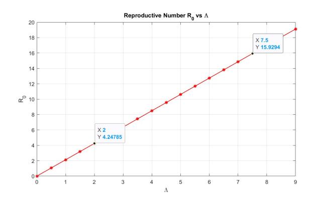
Figure 2: R0 value rises with an increase in vertical transmission Λ.
Figure 3 investigates how changes in the transmission rates from asymptomatic β1 and symptomatic β2 individuals affect the reproductive number R0. Both parameters are critical in disease spread since they govern how likely a susceptible individual is to become infected upon contact. The graph reveals that increasing either β1 or β2 results in a monotonic increase in R0, indicating higher disease transmissibility. Notably, the surface gradient is slightly steeper for β2, suggesting that transmission from symptomatic individuals has a slightly stronger influence on R0. This insight is important for public health interventions, as targeting symptomatic transmission (e.g., isolating symptomatic patients) could be more effective in reducing the spread.
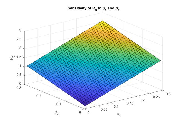
Figure 3: Sensitivity of R0 to transmission rates β1 and β2.
Figure 4 illustrates how the fraction of infected individuals who remain asymptomatic ρ and the overall rate of progression to infectiousness η influence R0. The parameter ρ modulates the division between asymptomatic and symptomatic pathways, while η represents the infectivity potential of newly exposed individuals. The surface shows a complex interaction R0 generally increases with η, but its response to ρ depends on η's value. For higher η, an increase in ρ (more asymptomatic cases) leads to a higher R0, reflecting the hidden risk of undiagnosed and untreated asymptomatic individuals sustaining the epidemic. This graph underscores the challenge of controlling Chlamydia, as a large proportion of infections may remain silent but still contribute to transmission.
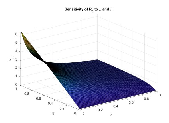
Figure 4: Sensitivity of R0 to asymptomatic fraction ρ and progression rate η.
Figure 5 explores the effect of the natural death rate µ and the latency period τ on the reproductive number.
The latency \(\tau\) appears in an exponential decay term, reducing the effective infectiousness with time by using condom, regular screening, partner limitation, and maintaining a healthy vaginal microbiome. The graph shows that \(\mathcal{R}_0\) decreases with increasing \(\tau\), reflecting how delays in becoming infectious reduce overall transmission potential. Conversely, the effect of \(\mu\) is more nuanced: for small \(\mu\), \(\mathcal{R}_0\) remains high, but as \(\mu\) increases, \(\mathcal{R}_0\) declines significantly due to reduced population turnover and a diminished infectious period. The surface sharply slopes downward for large \(\tau\) and \(\mu\), emphasizing that both natural mortality and delayed infectivity are key levers in reducing disease spread.
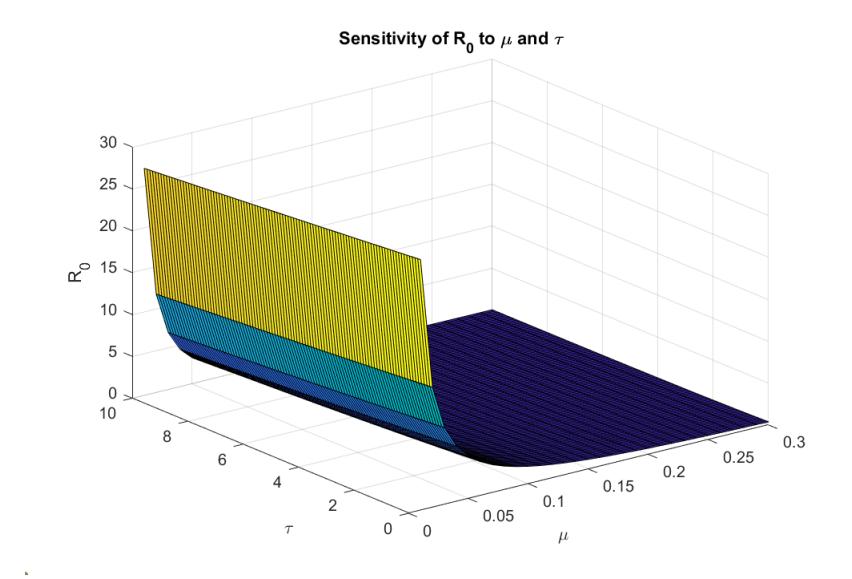
Figure 5: Effect of natural death rate \(\mu\) and exponential time delay factor \(\tau\) on \(\mathcal{R}_0\).
These four graphs collectively provide a visual and analytical understanding of how \(\mathcal{R}_0\) responds to changes in different epidemiological parameters. They help to identify which parameters have the most strongly influence on disease spread, guiding effective control and intervention strategies for Chlamydia.
5. STABILITY ANALYSIS
The stability at both locally and globally at the DF and EE points are examined in this section utilising the Routh-Hurwitz criterion and Lyapunov function with specific properties.
Theorem 5.1. The system's DF equilibrium point \((\varepsilon_0)\) is locally asymptotically stable when \(\mathcal{R}_0 < 1\).
Proof: It can be confirmed by linearizing the system around \(\varepsilon_0\), resulting in the following Jacobian matrix
\[J = \begin{bmatrix} -\mu & 0 & -\beta_1 \frac{\Lambda}{\mu} e^{-\mu\tau} & -\beta_2 \frac{\Lambda}{\mu} e^{-\mu\tau} & \alpha \\ 0 & -\rho\eta - \mu & \beta_1 \frac{\Lambda}{\mu} e^{-\mu\tau} & \beta_2 \frac{\Lambda}{\mu} e^{-\mu\tau} & 0 \\ 0 & -\rho\eta & -(r_1 + \mu) & 0 & 0 \\ 0 & \eta - \rho\eta & r_1 - \kappa r_1 & -r_2 - \mu & 0 \\ 0 & 0 & \kappa r_1 & r_2 & -(\mu + \alpha) \end{bmatrix}.\]
The corresponding eigenvalues are calculated by \(|J - \lambda I| = 0\)
\(\lambda_1 = -\mu < 0, \quad \lambda_2 = -(\mu + \alpha)\) and the roots of cubic equation.
The remaining three eigenvalues can be calculated by Routh-Hurwitz criteria.
\[J = \begin{vmatrix} -\rho \eta - \mu & \beta_1 \frac{\Lambda}{\mu} e^{-\mu \tau} & \beta_2 \frac{\Lambda}{\mu} e^{-\mu \tau} \\ \rho \eta & -r_1 - \mu - & 0 \\ \eta - \rho \eta & r_1 - \kappa r_1 & -r_2 - \mu - \end{vmatrix} = 0,\] by using the following characteristic equation
\[P(\lambda) = \lambda^3 - A_1 \lambda^2 + A_2 \lambda - A_3 = 0.\]
Suppose that,
\(A_1\)=Sum of diagonal, \(A_2\)=Sum of Co-diagonal and \(A_3\)=Determinant of J.
After finding the sum of diagonal, co-diagonal and determinant as mentioned above, we obtain
\[A_{1} = (\rho \eta + \mu) + (r_{1} + \mu) + (r_{2} + \mu).\] \[A_{2} = (r_{1} + \mu)(r_{2} + \mu) + (\rho \eta + \mu)(r_{2} + \mu) + (\rho \eta + \mu)(r_{1} + \mu) - \rho \eta \beta_{1} \frac{\Lambda}{\mu} e^{-\mu \tau}\] \[- \beta_{2} \frac{\Lambda}{\mu} (1 - \rho) \eta e^{-\mu \tau}.\] \[A_{3} = (\rho \eta + \mu)(r_{1} + \mu)(r_{2} + \mu)[1 - \mathcal{R}_{0}].\]
Hence, \(A_1 > 0\) and if \(\mathcal{R}_0 < 1\) then \(A_3 > 0\). Let
\[P = A_1 A_2 - A_3. (30)\]
Substituting \(A_1\), \(A_2\), and \(A_3\) obtained into P yield
\[P = [(\rho \eta + \mu) + (r_1 + \mu) + (r_2 + \mu)][(r_1 + \mu)(r_2 + \mu) + (\rho \eta + \mu)(r_2 + \mu) + (\rho \eta + \mu)(r_1 + \mu) - \rho \eta \beta_1 \frac{\Lambda}{\mu} e^{-\mu \tau} - \beta_2 \frac{\Lambda}{\mu} \eta e^{-\mu \tau} + \beta_2 \frac{\Lambda}{\mu} \rho \eta e^{-\mu \tau}] - [(\rho \eta + \mu)(r_1 + \mu)(r_2 + \mu) - \beta_1 \frac{\Lambda}{\mu} \rho \eta e^{-\mu \tau}(r_2 + \mu) - \beta_2 \frac{\Lambda}{\mu} \rho \eta e^{-\mu \tau}(1 - \kappa)r_1 - \beta_2 \frac{\Lambda}{\mu} \eta e^{-\mu \tau}(1 - \rho)(r_1 + \mu)].\]
Simplifying and splitting the expression of P into four compartments leads to
\[P = P(i) + P(ii) + P(iii) + P(iv),\] where
\[P(i) = ((\rho \eta + \mu)(\rho \eta + \mu)(r_1 + \mu) + (r_1 + \mu)(\rho \eta + \mu)(r_1 + \mu) - (\rho \eta + \mu)\rho \eta \beta_1 \frac{\Lambda}{\mu} e^{-\mu \tau} - (\rho \eta + \mu)\beta_2 \frac{\Lambda}{\mu} e^{-\mu \tau} \eta),\] \[P(ii) = ((\rho \eta + \mu)(\rho \eta + \mu)(r_1 + \mu) - (\rho \eta + \mu)\beta_2 \frac{\Lambda}{\mu} e^{-\mu \tau} \eta + (\rho \eta + \mu)\beta_2 \frac{\Lambda}{\mu} e^{-\mu \tau} \rho \eta + (r_2 + \mu) + (r_2 + \mu)(\rho \eta + \mu)(r_2 + \mu) - (r_2 + \mu)\beta_2 \frac{\Lambda}{\mu} e^{-\mu \tau} \eta + (r_2 + \mu)\beta_2 \frac{\Lambda}{\mu} e^{-\mu \tau} \rho \eta),\] \[P(iii) = (\beta_2 \frac{\Lambda}{\mu} e^{-\mu \tau} \rho \eta (1 - k)r_1),\]
\[\text{[rumus tidak dapat ditampilkan dengan baik — lihat PDF asli]}\]
Solving the first P(i), we obtain
\[(\rho \eta + \mu)(r_1 + \mu) \left[1 - \frac{\beta_1 \frac{\Lambda}{\mu} e^{-\mu \tau} \rho \eta}{(r_1 + \mu)(\rho \eta + \mu)}\right] (\rho \eta + 2\mu + r_1). \tag{31}\]
Solving the second P(ii), we have
\[(\rho \eta + \mu)(r_2 + \mu) \left[1 - \frac{\beta_2 \frac{\Lambda}{\mu} e^{-\mu \tau} \eta (1 - \rho)}{(r_2 + \mu)(\rho \eta + \mu)}\right] (\rho \eta + 2\mu + r_2). \tag{32}\]
The third compartment P(iii) is already in reduced. Solving the fourth compartment P(iv), we have
\[(r_1 + \mu)(r_2 + \mu)[r_1 + r_2 + 2\rho\eta + 4\mu]. \tag{33}\]
Combining all results, the main solution for P is
\[A_{1}A_{2} - A_{3} = (\rho \eta + \mu)(r_{1} + \mu) \left[ 1 - \frac{\beta_{1} \frac{\Lambda}{\mu} e^{-\mu \tau} \rho \eta}{(\rho \eta + \mu)(r_{1} + \mu)} (\rho \eta + 2\mu + r_{1}) \right]\] \[+ (\rho \eta + \mu)(r_{2} + \mu) \left[ 1 - \frac{\beta_{2} \frac{\Lambda}{\mu} e^{-\mu \tau} \eta (1 - \rho)}{(r_{2} + \mu)(\rho \eta + \mu)} \right] (\rho \eta + 2\mu + r_{2})\] \[+ \beta_{2} \frac{\Lambda}{\mu} e^{-\mu \tau} \rho \eta (1 - \kappa) r_{1} + (r_{1} + \mu)(r_{2} + \mu) [r_{1} + r_{2} + 2\rho \eta + 4\mu].\] \[(34)\]
Notice that if
\[\mathcal{R}_0 < 1 \text{ then } \tfrac{\beta_1 \frac{\Lambda}{\mu} e^{-\mu \tau} \rho \eta}{(\rho \eta + \mu)(r_1 + \mu)} < 1 \text{ and } \tfrac{\beta_2 \frac{\Lambda}{\mu} e^{-\mu \tau} \eta (1 - \rho)}{(r_2 + \mu)(\rho \eta + \mu)} < 1,\] which implies that if \(\mathcal{R}_0 < 1\) then \(A_1 A_2 - A_3 > 0\).
Consequently, according to the Routh-Hurwitz criterion, if \(\mathcal{R}_0 < 1\), then \(P(\lambda) = 0\) has negative real roots, i.e. the system of differential equations represents local asymptotic stability at \(E_0\) when \(\mathcal{R}_0 < 1\). This completes the proof. Hence proves that all eigenvalues are negative so, \(E_0\) proves the local asymptotic stability.
Theorem 5.2. If \(\mathcal{R}_0 > 1\), the EE points \((\varepsilon_1)\) of the model's solution are locally asymptotically stable.
Proof: Linearizing a system around \(\varepsilon_1\), the corresponding Jacobian matrix is as follows
\[J = \begin{bmatrix} -\beta_1 I_A^* e^{-\mu\tau} - \beta_1 I_S^* e^{-\mu\tau} - \mu & 0 & -\beta_1 S^* e^{-\mu\tau} & -\beta_2 S^* e^{-\mu\tau} & \alpha \\ \beta_1 I_A^* e^{-\mu\tau} + \beta_2 I_S^* e^{-\mu\tau} & -(\eta + \mu) & \beta_1 S^* e^{-\mu\tau} & \beta_2 S^* e^{-\mu\tau} & 0 \\ 0 & \rho\eta & -(r_1 + \mu) & 0 & 0 \\ 0 & \eta(1 - \rho) & (1 - \kappa)r_1 & -(r_2 + \mu) & 0 \\ 0 & 0 & \kappa r_1 & r_2 & -(\mu + \alpha) \end{bmatrix}.\]
The matrix J is then converted into the following symbolic form
\[J = \begin{bmatrix} b_{11} & b_{12} & b_{13} & b_{14} & b_{15} \\ b_{21} & b_{22} & b_{23} & b_{24} & b_{25} \\ b_{31} & b_{32} & b_{33} & b_{34} & b_{35} \\ b_{41} & b_{42} & b_{43} & b_{44} & b_{45} \\ b_{51} & b_{52} & b_{53} & b_{54} & b_{55} \end{bmatrix},\]
upon which the characteristic equation of \(J(\varepsilon_1)\) is given by,
\[\lambda^5 + G_1 \lambda^4 + G_2 \lambda^3 + G_3 \lambda^2 + G_4 \lambda + G_5 = 0.\] (35)
where
\[G_1 = -b_{11} - b_{22} - b_{33} - b_{44} - b_{55}\]
\[\text{[rumus tidak dapat ditampilkan dengan baik — lihat PDF asli]}\]
\(b_{23}b_{32}b_{43}\),
\(\text{[rumus tidak dapat ditampilkan dengan baik — lihat PDF asli]}\)\(\text{[rumus tidak dapat ditampilkan dengan baik — lihat PDF asli]}\)\(b_{11}b_{24}b_{42}b_{55} - b_{24}b_{33}b_{42}b_{55} - b_{11}b_{24}b_{33}b_{42} - b_{14}b_{21}b_{32}b_{43} - b_{15}b_{21}b_{32}b_{53} - b_{15}b_{21}b_{42}b_{54},\)
\(\text{[rumus tidak dapat ditampilkan dengan baik — lihat PDF asli]}\)\(b_{13}b_{21}b_{32}b_{44}b_{55} - b_{15}b_{21}b_{32}b_{43}b_{54} - b_{11}b_{23}b_{32}b_{43}b_{55} - b_{14}b_{21}b_{33}b_{42}b_{55}.\)
According to the Routh-Hurwitz criterion, all eigenvalues of the characteristic equation contain negative real parts if and only if \(G_i > 0\) (i = 1, 2, 3, 4, 5),
\[\begin{split} D_1 &> 0, \quad D_2 = \begin{vmatrix} G_1 & G_3 \\ 1 & G_2 \end{vmatrix} = G_1 G_2 - G_3 > 0, \\ D_3 &= \begin{vmatrix} G_1 & G_3 & G_5 \\ 1 & G_2 & G_4 \\ 0 & G_1 & G_3 \end{vmatrix} = G_1 G_2 G_3 - G_1^2 G_4 - G_3^2 + G_1 G_5 > 0, \\ D_4 &= \begin{vmatrix} G_1 & G_3 & G_5 & 0 \\ 1 & G_2 & G_4 & 0 \\ 0 & G_1 & G_3 & G_5 \\ 0 & 1 & G_2 & G_4 \end{vmatrix} = D_2 (G_3 G_4 - G_2 G_5) - (G_1 G_4 - G_5)^2 > 0, \\ D_5 &= \begin{vmatrix} G_1 & G_3 & G_5 & 0 & 0 \\ 1 & G_2 & G_4 & 0 & 0 \\ 0 & G_1 & G_3 & G_5 & 0 \\ 0 & 1 & G_2 & G_4 & 0 \\ 0 & 0 & G_1 & G_3 & G_5 \end{vmatrix}, \end{split}\]
\[D_5 = G_1 G_4 G_5 (G_2 G_3 - G_1 G_4) - G_1 G_2^2 G_5^2 + G_1 G_4 G_5^2 - G_4 G_5 (G_3^2 - G_1 G_5) + G_2 G_3 G_5^2 - G_5^2 > 0.\]
Hence, the system demonstrates local asymptotic stability when \(\mathcal{R}_0 > 1\) and all above conditions are satisfied. This concludes the proof.
Theorem 5.3. The Chlamydia-free points \(\varepsilon_0 = \left(\frac{\Lambda}{\mu}, 0, 0, 0\right)\) of the system is globally asymptotically stable (GAS) when \(\mathcal{R}_0 < 1\) and is unstable when \(\mathcal{R}_0 > 1\).
Proof: Take into account a Volterra-type Lyapunov function U \(\Omega \to \mathbb{R}\)
\[U = S - S^0 \ln S + E + I_A + I_S.\]
Taking the time derivative of U,
\[\dot{U} = \left(1 - \frac{S^0}{S}\right)\dot{S} + \dot{E} + \dot{I}_A + \dot{I}_S,\] and substituting \(S, E, I_A, I_S\) into the derivative yield,
\[\begin{split} \dot{U} &= \left(1 - \frac{S^0}{S}\right) \left[\Lambda - \beta_1 S I_A e^{-\mu \tau} - \beta_2 S I_S e^{-\mu \tau} - \mu S + \alpha R\right] \\ &+ \left[\beta_1 S I_A e^{-\mu \tau} + \beta_2 S I_S e^{-\mu \tau} - \rho \eta E - \mu E\right] + \left[\rho \eta E - (r_1 + \mu) I_A\right] \\ &+ \left[(1 - \rho) \eta E + (1 - \kappa) r_1 I_A - (r_2 + \mu) I_S(t)\right]. \end{split}\]
Rearranging the terms,
\[\dot{U} = \Lambda - \mu S + \alpha R - \frac{S^0}{S} \Lambda + \frac{S^0}{S} \beta_1 S I_A e^{-\mu \tau} + \frac{S^0}{S} \beta_2 S I_S e^{-\mu \tau} + \frac{S^0}{S} \mu S - \frac{S^0}{S} \alpha R - (\rho \eta + \mu + \eta) E - (\kappa r_1 + \mu) I_A - (r_2 + \mu) I_S,\]
letting \(\Lambda = \mu S^0\) and simplifying, we obtain,
\[\dot{U} = -\frac{\mu}{S}(S-S^0)^2 + (\frac{\Lambda}{\mu}\beta_1 S e^{-\mu\tau} - (\kappa r_1 + \mu))I_A + (\frac{\Lambda}{\mu}\beta_2 S e^{-\mu\tau} - (r_2 + \mu))I_S - (\rho\eta + \mu + \eta)E - \frac{\Lambda}{\mu S}R.\]
\[\frac{\Lambda}{\mu}\beta_1 S e^{-\mu\tau} < (\kappa r_1 + \mu),\]
we have \(\dot{U} \leq 0\) for \(\mathcal{R}_0 < 1\). Moreover, if \(\mathcal{R}_0 < 1\), then \(\dot{U} = 0\). That is equal to \(S = S^0, E = 0, I_A = 0, I_S = 0, R = 0\), whereas \(\dot{U} = 0 \quad \forall (S, E, I_A, I_S, R) \neq (S^0, 0, 0, 0, 0)\).
Theorem 5.4. For \(\mathcal{R}_0 > 1\), the system is globally asymptotically stable at the indicated point \(\varepsilon_1\).
Proof: Consider a Volterra-type Lyapunov function \(V \Omega \to \mathbb{R}\).
The following Lyapunov function is proposed as a candidate to demonstrate the system's global stability at EE points \(\varepsilon_1\), defined by the relation
\[V = X_1 [S - S^* \ln S] + X_2 [E - E^* \ln E] + X_3 [I_A - I_A^* \ln I_A] + X_4 [I_S - I_S^* \ln I_S],\] where \(X_1, X_2, X_3\) and \(X_4\) are positive constants to be determined subsequently.
Then,
\[\dot{V} = X_1 \left( 1 - \frac{S^*}{S} \right) \dot{S} + X_2 \left( 1 - \frac{E^*}{E} \right) \dot{E} + X_3 \left( 1 - \frac{I_A^*}{I_A} \right) \dot{I_A} + X_4 \left( 1 - \frac{I_S^*}{I_S} \right) \dot{I_S}.\]
By inserting the time derivative of models equation. We have,
\[\dot{V} = X_1 \left( 1 - \frac{S^*}{S} \right) \left[ \Lambda - \beta_1 S I_A e^{-\mu \tau} - \beta_2 S I_S e^{-\mu \tau} - \mu S + \alpha R \right] + X_2 \left( 1 - \frac{E^*}{E} \right) \left[ \beta_1 S I_A e^{-\mu \tau} + \beta_2 S I_S(t) e^{-\mu \tau} - \rho \eta E - \mu E \right] + X_3 \left( 1 - \frac{I_A^*}{I_A} \right) \left[ \rho \eta E - (r_1 + \mu) I_A \right] + X_4 \left( 1 - \frac{I_S^*}{I_S} \right) \left[ (1 - \rho) \eta E + (1 - \kappa) r_1 I_A - (r_2 + \mu) I_S \right].\]
After simplification
\[\begin{split} \dot{V} &= X_{1} \left( S - S^{*} \right) \left[ \frac{\Lambda}{S} - \beta_{1} I_{A} e^{-\mu \tau} - \beta_{2} I_{S} e^{-\mu \tau} - \mu + \frac{\alpha R}{S} \right] + \\ X_{2} \left( E - E^{*} \right) \left[ \frac{\beta_{1} S I_{A} e^{-\mu \tau}}{E} + \frac{\beta_{2} S I_{S} (t) e^{-\mu \tau}}{E} - \rho \eta - \mu \right] + \\ X_{3} \left( I_{A} - I_{A}^{*} \right) \left[ \frac{\rho \eta E}{I_{A}} - \left( r_{1} + \mu \right) \right] + \\ X_{4} \left( I_{S} - I_{S}^{*} \right) \left[ \frac{(1 - \rho) \eta E}{I_{S}} + \frac{(1 - \kappa) r_{1} I_{A}}{I_{S}} - \left( r_{2} + \mu \right) \right]. \end{split}\]
Since,
\[\varepsilon_1 = (S^*, E^*, I_A^*, I_S^*),\] from the system, we have
\[\frac{dS^*}{dt} = \frac{dE^*}{dt} = \frac{dI_A^*}{dt} = \frac{dI_S^*}{dt} = 0.\]
Let
\[\mu = \frac{\Lambda}{S_*} - \beta_1 I_A^* e^{-\mu \tau} - \beta_2 I_S^* e^{-\mu \tau} + \frac{\alpha R}{S^*},\]
\[\rho \eta + \mu = \frac{(\beta_1 S^* I_A^* e^{-\mu \tau}) + (\beta_2 S^* I_S^* e^{-\mu \tau})}{E},\]
\[r_1 + \mu = \frac{\rho \eta E^*}{I_A^*},\]
\[r_2 + \mu = \frac{(\eta E^* - \rho \eta E^*) + (r_1 I_A^* - \kappa r_1 I_A^*)}{I_S^*},\]
we then have
\[\begin{split} \dot{V} &= X_1 \left( S - S^* \right) \left[ \frac{\Lambda}{S} - \beta_1 I_A e^{-\mu \tau} - \beta_2 I_S e^{-\mu \tau} - \left( \frac{\Lambda}{S_*} - \beta_1 I_A^* e^{-\mu \tau} - \beta_2 I_S^* e^{-\mu \tau} + \frac{\alpha R}{S} \right) + \frac{\alpha R}{S} \right] + \\ X_2 \left( E - E^* \right) \left[ \frac{\beta_1 S I_A e^{-\mu \tau}}{E} + \frac{\beta_2 S I_S (t) e^{-\mu \tau}}{E} - \left( \frac{\beta_1 S^* I_A^* e^{-\mu \tau}}{E^*} + \frac{\beta_2 S^* I_S^* (t) e^{-\mu \tau}}{E^*} \right) \right] + \\ X_3 \left( I_A - I_A^* \right) \left[ \frac{\rho \eta E}{I_A} - \frac{\rho \eta E^*}{I_A^*} \right] + \\ X_4 \left( I_S - I_S^* \right) \left[ \frac{(1 - \rho) \eta E}{I_S} + \frac{(1 - \kappa) r_1 I_A}{I_S} - \left( \frac{(1 - \rho) \eta E^*}{I_S^*} + \frac{(1 - k) r_1 I_A^*}{I_S^*} \right) \right]. \end{split}\]
For
\[X_1 = X_2 = X_3 = X_4 = 1,\]
we have.
\[\dot{V} = -\Lambda \frac{(S - S^*)^2}{SS^*} \le 0.\]
Therefore, V is confirmed to be a Lyapunov function and \(\varepsilon_1\) is globally asymptotically stable.
NUMERICAL ANALYSIS
The dynamical behavior of the system is investigated using two finite difference schemes Euler's integration and the RK-4, along with the NSFD approach.
6.1. Forward Euler's Finite Difference Method
\[S^{n+1} = S^n + h(\Lambda - \beta_1 S^n I_A^n e^{-\mu \tau} - \beta_2 S^n I_S^n e^{-\mu \tau} - \mu S^n + \alpha R^n), \tag{36a}\]
\[E^{n+1} = E^n + h(\beta_1 S^n I_A^n e^{-\mu \tau} + \beta_2 S^n I_S^n e^{-\mu \tau} - \rho \eta E^n - \mu E^n), \tag{36b}\]
\[I_A^{n+1} = I_A^n + h(\rho \eta E^n - (r_1 + \mu)I_A^n),\] \[I_S^{n+1} = I_S^n + h((1 - \rho)\eta E^n + (1 - \kappa)r_1I_A^n - (r_2 + \mu)I_S^n),\] (36d)
\[I_S^{n+1} = I_S^n + h((1-\rho)\eta E^n + (1-\kappa)r_1 I_A^n - (r_2 + \mu)I_S^n), \tag{36d}\]
\[R^{n+1} = R^n + h(\kappa r_1 I_A^n + r_2 I_S^n - \mu R^n - \alpha R^n), \tag{36e}\] where h is any step size.
6.2. RK4 Method
Here by \(SEI_AI_SR\) system to develop an explicit RK4 method
\[S^{n+1} = S^n + \frac{1}{6}[K_1 + 2K_2 + 2K_3 + K_4]\] (37a)
\[E^{n+1} = E^n + \frac{1}{6}[L_1 + 2L_2 + 2L_3 + L_4]\] (37b)
\[I_A^{n+1} = I_A^n + \frac{1}{6}[M_1 + 2M_2 + 2M_3 + M_4]\] (37c)
\[I_S^{n+1} = I_S^n + \frac{1}{6}[N_1 + 2N_2 + 2N_3 + N_4]\] (37d)
\[R^{n+1} = R^n + \frac{1}{6}[O_1 + 2O_2 + 2O_3 + O_4]\] (37e)
h is step size and \(n = 0, 1, 2, 3, 4 \dots\), where
\[\begin{split} K_1 &= h \left[ \Lambda - \beta_1 S^n I_A^n e^{-\mu \tau} - \beta_2 S^n I_S^n e^{-\mu \tau} - \mu S^n + \alpha R^n \right], \\ L_1 &= h \left[ \beta_1 S^n I_A^n e^{-\mu \tau} + \beta_2 S^n I_S^n e^{-\mu \tau} - \rho \eta E^n - \mu E^n \right], \\ M_1 &= h \left[ \rho \eta E^n - (r_1 + \mu) I_A^n \right], \\ N_1 &= h \left[ (1 - \rho) \eta E^n + (1 - \kappa) r_1 I_A^n - (r_2 + \mu) I_S^n \right], \\ O_1 &= h \left[ \kappa r_1 I_A^n + r_2 I_S^n - \mu R^n - \alpha R^n \right]. \end{split}\]
\[\text{[rumus tidak dapat ditampilkan dengan baik — lihat PDF asli]}\]
\[\begin{split} K_4 &= h \left[ \Lambda - \beta_1 (S^n + K_3) (I_A^n + M_3) e^{-\mu\tau} - \beta_2 (S^n + K_3) (I_S^n + N_3) e^{-\mu\tau} - \mu (S^n + K_3) + \alpha (R^n + O_3) \right], \\ L_4 &= h \left[ \beta_1 (S^n + K_3) (I_A^n + M_3) e^{-\mu\tau} + \beta_2 (S^n + K_3) (I_S^n + N_3) e^{-\mu\tau} - \rho \eta (E^n + L_3) - \mu (E^n + L_3) \right], \\ M_4 &= h \left[ \rho \eta (E^n + L_3) - (r_1 + \mu) (I_A^n + M_3) \right], \\ N_4 &= h \left[ (1 - \rho) \eta (E^n + L_3) + (1 - \kappa) r_1 (I_A^n + M_3) - (r_2 + \mu) (I_S^n + N_3) \right], \\ O_4 &= h \left[ \kappa r_1 (I_A^n + M_3) + r_2 (I_S^n + N_3) - \mu (R^n + O_3) - \alpha (R^n + O_3) \right]. \end{split}\]
6.3. NSFD Method
Convergence results of NSFD are proved for our model in below explanation. Also in this section, we will look about the stability of NSFD method at the DFE of \(SEI_AI_SR\) model.
\[\frac{S^{n+1} - S^n}{h} = \Lambda - \beta_1 S^{n+1} I_A^n e^{-\mu \tau} - \beta_2 S^{n+1} I_S^n e^{-\mu \tau} - \mu S^{n+1} + \alpha R^n,\]
here, h is step size and n is number of iterations as n = 0, 1, 2, 3, 4..., after simplification,
\[S^{n+1} = \frac{S^n + h\Lambda + h\alpha R^n}{1 + h\beta_1 I_A^n e^{-\mu\tau} + h\beta_2 I_S^n e^{-\mu\tau} + h\mu},\] (38a)
\[E^{n+1} = \frac{E^n + h\beta_1 S^n I_A^n e^{-\mu\tau} + h\beta_2 S^n I_S^n e^{-\mu\tau}}{1 + h\rho\eta + h\mu},\] (38b)
\[I_A^{n+1} = \frac{I_A^n + h\rho\eta E^n}{1 + h(r_1 + \mu)},\tag{38c}\]
\[I_S^{n+1} = \frac{I_S^n + h(1-\rho)\eta E^n + h(1-\kappa)r_1 I_A^n}{1 + h(r_2 + \mu)},\] (38d)
\[I_S^{n+1} = \frac{I_S^n + h(1-\rho)\eta E^n + h(1-\kappa)r_1 I_A^n}{1 + h(r_2 + \mu)},\] \[R^{n+1} = \frac{R^n + h\kappa r_1 I_A^n + hr_2 I_S^n}{1 + h\mu + h\alpha}.\] (38d)
6.4. Convergence Analysis of NSFD Method
In this segment, convergence analysis of the NSFD method will be carried out at the DF points \(\varepsilon_0 = (\frac{\Lambda}{\mu}, 0, 0, 0, 0)\).
\[\begin{split} C &= S^{n+1} = \frac{S + h\Lambda + h\alpha R}{1 + h\beta_1 I_A e^{-\mu\tau} + h\beta_2 I_S e^{-\mu\tau} + h\mu}, \quad D = E^{n+1} = \frac{E + h\beta_1 S I_A e^{-\mu\tau} + h\beta_2 S I_S e^{-\mu\tau}}{1 + h\rho\eta + h\mu}, \\ F &= I_A^{n+1} = \frac{I_A + h\rho\eta E}{1 + h(r_1 + \mu)}, \quad G = I_S^{n+1} = \frac{I_S + h(1 - \rho)\eta E + h(1 - \kappa)r_1 I_A}{1 + h(r_2 + \mu)}, \\ H &= R^{n+1} = \frac{R + h\kappa r_1 I_A + hr_2 I_S}{1 + h\mu + h\alpha}. \end{split}\]
Differentiating C,D,F,G and H with respect to S,E,\(I_A\),\(I_S\) and R, we obtain the Jacobian matrix of the equations,
\[J = \begin{bmatrix} C_S & C_E & C_{I_A} & C_{I_S} & C_R \\ D_S & D_E & D_{I_A} & D_{I_S} & D_R \\ F_S & F_E & F_{I_A} & F_{I_S} & F_R \\ G_S & G_E & G_{I_A} & G_{I_S} & G_R \\ H_S & H_E & H_{I_A} & H_{I_S} & H_R \end{bmatrix}.\]
Substituting the values, the Jacobian matrix becomes
\[J = \begin{bmatrix} \frac{1}{1+h\mu} & 0 & \frac{-h\beta_1 e^{-\mu\tau} \left(\frac{\Lambda}{\mu} + h\Lambda\right)}{(1+h\mu)^2} & \frac{-h\beta_2 e^{-\mu\tau} \left(\frac{\Lambda}{\mu} + h\Lambda\right)}{(1+h\mu)^2} & \frac{h\alpha}{1+h\mu} \\ 0 & \frac{1}{1+h\rho\eta + h\mu} & \frac{h\beta_1 \frac{\Lambda}{\mu} e^{-\mu\tau}}{1+h\rho\eta + h\mu} & \frac{h\beta_2 \frac{\Lambda}{\mu} e^{-\mu\tau}}{1+h\rho\eta + h\mu} & 0 \\ 0 & \frac{h\rho\eta}{1+h(r_1 + \mu)} & \frac{1}{1+h(r_1 + \mu)} & 0 & 0 \\ 0 & \frac{h\eta(1-\rho)}{1+h(r_2 + \mu)} & \frac{hr_1(1-\kappa)}{1+h(r_2 + \mu)} & \frac{1}{1+h(r_2 + \mu)} & 0 \\ 0 & 0 & \frac{h\kappa r_1}{1+h\mu + h\alpha} & \frac{hr_2}{1+h\mu + h\alpha} & \frac{1}{1+h\mu + h\alpha} \end{bmatrix}\] \[det(J - \lambda I) = 0\] \[\begin{vmatrix} \lambda - F_1 & 0 & F_2 & F_3 & F_4 \\ 0 & \lambda - F_5 & F_6 & F_7 & 0 \\ 0 & F_8 & \lambda - F_9 & 0 & 0 \\ 0 & F_{10} & F_{11} & \lambda - F_{12} & 0 \\ 0 & 0 & F_{13} & F_{14} & \lambda - F_{15} \end{vmatrix} = 0.\]
Expanding by \(C_1\),
\[(\lambda - F_1) \begin{vmatrix} \lambda - F_5 & F_6 & F_7 & 0 \\ F_8 & \lambda - F_9 & 0 & 0 \\ F_{10} & F_{11} & \lambda - F_{12} & 0 \\ 0 & F_{13} & F_{14} & \lambda - F_{15} \end{vmatrix} = 0.\]
Expanding by \(C_4\),
\[(\lambda - F_1)(\lambda - F_{15}) \begin{vmatrix} \lambda - F_5 & F_6 & F_7 \\ F_8 & \lambda - F_9 & 0 \\ F_{10} & F_{11} & \lambda - F_{12} \end{vmatrix} = 0.\]
Therefore, the eigenvalues \(\lambda_1 = F_1\) and \(\lambda_2 = F_{15}\). The other three eigenvalues will be obtained from
\[\begin{vmatrix} \lambda - F_5 & F_6 & F_7 \\ F_8 & \lambda - F_9 & 0 \\ F_{10} & F_{11} & \lambda - F_{12} \end{vmatrix} = 0.\]
Schur-Cohn Stability Conditions Regarding the characteristic polynomial \(Q(\lambda) = \lambda^3 + A_1 \lambda^2 + A_2 \lambda + A_3\) having solutions \(\lambda_i\): j=1,2,3 of equation Q(\(\lambda\))=0 satisfy \(|\eta_i| < 1\) if the following criteria met.
1. \[Q(1)=1 + A_1 + A_2 + A_3 > 0\], 1. \[Q(1)=1 + A_1 + A_2 + A_3 > 0\],
2. \((-1)^3 Q(-1)=1 - A_1 + A_2 - A_3 > 0\),
3. \(1 - (A_3)^2 > |A_2 - A_1 A_3|\).
3. \[1 - (A_3)^2 > |A_2 - A_1 A_3|\].
Let, the characteristic polynomial of above Jacobian is which implies that
\[\lambda^3 - \lambda^2 (F_{12} + F_9 + F_5) + \lambda (F_9 F_{12} + F_5 F_{12} + F_5 F_9 - F_{10} F_7 - F_6 F_8) + (-F_5 F_9 F_{12} + F_7 F_8 F_{11} + F_{10} F_7 F_9 + F_6 F_8 F_{12}) = 0\]
The above expression can be expressed in a more simplified form as
\[\lambda^3 + A_1 \lambda^2 + A_2 \lambda + A_3 = 0\],
\[A_1\]=-(\(F_{12}\)+ \(F_9\)+\(F_5\)), \(A_2\)=(\(F_9F_{12}\)+ \(F_5F_{12}\)+ \(F_5F_9\)-\(F_{10}F_7\)- \(F_6F_8\)) and \(A_3\)= (-\(F_5F_9F_{12}\)+\(F_7F_8F_{11}\)+\(F_{10}F_7F_9\)+\(F_6F_8F_{12}\)).
Clearly, the first and second eigenvalues are
\[\lambda_1=F_1=\frac{1}{1+h\mu}<1\] and \(\lambda_2=F_{15}=\frac{1}{(1+h\mu+h\alpha)}<1\).
For other eigenvalues, we choose \(\lambda^3 + A_1 \lambda^2 + A_2 \lambda + A_3 = 0\).
\[A_1\]=-(\(F_{12}\)+ \(F_9\)+\(F_5\)), \(A_2\)= (\(F_9F_{12}\)+ \(F_5F_{12}\)+ \(F_5F_9\)-\(F_{10}F_7\)- \(F_6F_8\)) and \(A_3\)= (-\(F_5F_9F_{12}\)+\(F_7F_8F_{11}\)+\(F_{10}F_7F_9\)+\(F_6F_8F_{12}\))
After simplification, we have
- Q(1)=1 + \(A_1\) + \(A_2\) + \(A_3\), \((-1)^3\) Q(-1)=\((-1)^3\) Q(-1)=1 \(A_1\) + \(A_2\) \(A_3\), \(1 (A_3)^2 > |A_2 A_1 A_3|\).
Hence, by calculation the above three conditions are satisfied. Thus, all the eigenvalues are inside the unit circle by Schur-Cohn Stability Conditions and our developed NSFD scheme is local asymptotically stable, confirmed by this theorem.
6.5. Consistency Analysis
The consistency of the numerical method is analyzed using Taylor series expansion. Initially, we select the first equation from the numerical integration model and apply expansion of Taylor's series to \(S^{n+1}\)
\[S^{n+1} = S^n + h \frac{dS}{dt} + \frac{h^2}{2!} \frac{d^2S}{dt^2} + \frac{h^3}{3!} \frac{d^3S}{dt^3} + \dots\] (39)
In the subsequent expression
\[S^{n+1}(1+h\beta_{1}I_{A}^{n}e^{-\mu\tau}+h\beta_{2}I_{S}^{n}e^{-\mu\tau}+h\mu) = S^{n}+h\Lambda+h\alpha R^{n},\] \[\left(S^{n}+h\frac{dS}{dt}+\frac{h^{2}}{2!}\frac{d^{2}S}{dt^{2}}+\frac{h^{3}}{3!}\frac{d^{3}S}{dt^{3}}+\cdots\right)(1+h\beta_{1}I_{A}^{n}e^{-\mu\tau}+h\beta_{2}I_{S}^{n}e^{-\mu\tau}+h\mu) = S^{n}+h\Lambda+h\alpha R^{n},\] \[S^{n}+hS^{n}\beta_{1}I_{A}^{n}e^{-\mu\tau}+hS^{n}\beta_{2}I_{S}^{n}e^{-\mu\tau}+S^{n}h\mu+h\frac{dS}{dt}+h^{2}\frac{dS}{dt}\beta_{1}I_{A}^{n}e^{-\mu\tau}+h^{2}\frac{dS}{dt}\beta_{2}I_{S}^{n}e^{-\mu\tau}+h^{2}\mu\frac{dS}{dt}\] \[+\left(\frac{h^{2}}{2!}\frac{d^{2}S}{dt^{2}}+\frac{h^{3}}{3!}\frac{d^{3}S}{dt^{3}}+\cdots\right)(1+h\beta_{1}I_{A}^{n}e^{-\mu\tau}+h\beta_{2}I_{S}^{n}e^{-\mu\tau}+h\mu) = S^{n}+h\Lambda+h\alpha R^{n},\] \[h\left(S^{n}\beta_{1}I_{A}^{n}e^{-\mu\tau}+S^{n}\beta_{2}I_{S}^{n}e^{-\mu\tau}+S^{n}\mu+\frac{dS}{dt}+h\frac{dS}{dt}\beta_{1}I_{A}^{n}e^{-\mu\tau}+h\frac{dS}{dt}\beta_{2}I_{S}^{n}e^{-\mu\tau}+h\mu\frac{dS}{dt}\right)\] \[+\left(\frac{h}{2!}\frac{d^{2}S}{dt^{2}}+\frac{h^{2}}{3!}\frac{d^{3}S}{dt^{3}}+\cdots\right)(1+h\beta_{1}I_{A}^{n}e^{-\mu\tau}+h\beta_{2}I_{S}^{n}e^{-\mu\tau}+h\mu) = h(\Lambda+\alpha R^{n}), \quad (40)\]
Simplifying the terms yield
\[S^{n}\beta_{1}I_{A}^{n}e^{-\mu\tau} + S^{n}\beta_{2}I_{S}^{n}e^{-\mu\tau} + S^{n}\mu + \frac{dS}{dt} + h\frac{dS}{dt}\beta_{1}I_{A}^{n}e^{-\mu\tau} + h\frac{dS}{dt}\beta_{2}I_{S}^{n}e^{-\mu\tau} + h\mu\frac{dS}{dt} + \left(\frac{h}{2!}\frac{d^{2}S}{dt^{2}} + \frac{h^{2}}{3!}\frac{d^{3}S}{dt^{3}} + \cdots\right)(1 + h\beta_{1}I_{A}^{n}e^{-\mu\tau} + h\beta_{2}I_{S}^{n}e^{-\mu\tau} + h\mu) = \Lambda + \alpha R^{n}.\](41)
By taking the limit as \(h \to 0\), we obtain
\[S^{n}\beta_{1}I_{A}^{n}e^{-\mu\tau} + S^{n}\beta_{2}I_{S}^{n}e^{-\mu\tau} + S^{n}\mu + \frac{dS}{dt} = \Lambda + \alpha R^{n},\] \[\Longrightarrow \frac{dS}{dt} = \Lambda + \alpha R^{n} - S^{n}\beta_{1}I_{A}^{n}e^{-\mu\tau} - S^{n}\beta_{2}I_{S}^{n}e^{-\mu\tau} - S^{n}\mu.\] (42)
According to this result, the discretized equation we derived aligns with Equation (2a) of the system. Likewise, we consider Equation (2b) and by the Taylor series expansion on \(E^{n+1}\).
\[E^{n+1} = E^n + h\frac{dE}{dt} + \frac{h^2}{2!}\frac{d^2E}{dt^2} + \frac{h^3}{3!}\frac{d^3E}{dt^3} + \dots\] (43)
Similarly, we have
\[E^{n+1}(1 + h\rho\eta + h\mu) = E^n + h\beta_1 S^n I_A^n e^{-\mu\tau} + h\beta_2 S^n I_S^n e^{-\mu\tau}, \tag{44}\]
\[E^{n}h\rho\eta + E^{n}h\mu + h\frac{dE}{dt} + h^{2}\frac{dE}{dt}\rho\eta + h^{2}\frac{dE}{dt}\mu + \left(\frac{h}{2!}\frac{d^{2}E}{dt^{2}} + \frac{h^{2}}{3!}\frac{d^{3}E}{dt^{3}} + \cdots\right) \times (1 + h\rho\eta + h\mu) = h\beta_{1}S^{n}I_{A}^{n}e^{-\mu\tau} + h\beta_{2}S^{n}I_{S}^{n}e^{-\mu\tau}.\] (45)
By applying \(h \to 0\), we obtain
\[\frac{dE}{dt} = \beta_1 S^n I_A^n e^{-\mu \tau} + \beta_2 S^n I_S^n e^{-\mu \tau} - \rho \eta E^n - \mu E^n.\] (46)
Applying Taylor's series expansion of \(I_A^{n+1}\) from Equations (2c), (2d), and (2e) and simplifying, we obtain Equations (47), (49), and (51), respectively. Applying \(h \to 0\) on them respectively yield Equations (48), (50), and (52).
\[r_{1}I_{A}^{n} + \mu I_{A}^{n} + \frac{dI_{A}}{dt} + h\frac{dI_{A}}{dt}r_{1} + h\frac{dI_{A}}{dt}\mu + \left(\frac{h}{2!}\frac{d^{2}I_{A}}{dt^{2}} + \frac{h^{2}}{3!}\frac{d^{3}I_{A}}{dt^{3}} + \cdots\right) \times (1 + hr_{1} + h\mu) = \rho \eta E^{n}.\] \[(47)\]
\[\frac{dI_A^n}{dt} = \rho \eta E^n - r_1 I_A^n - \mu I_A^n. \tag{48}\]
\[I_S^n r_2 + \mu I_S^n + \frac{dI_S}{dt} + h \frac{dI_S}{dt} r_2 + h \frac{dI_S}{dt} \mu + \left(\frac{h}{2!} \frac{d^2 I_S}{dt^2} + \frac{h^2}{3!} \frac{d^3 I_S}{dt^3} + \cdots\right) \times (1 + hr_2 + h\mu) = (1 - \rho) \eta E^n + (1 - \kappa) r_1 I_A^n.\] \[(49)\]
\[\frac{dI_S}{dt} = (1 - \rho)\eta E^n + (1 - \kappa)r_1 I_A^n - r_2 I_S^n - \mu I_S^n.\] (50)
\[R^{n}\mu + R^{n}\alpha + \frac{dR}{dt} + h\frac{dR}{dt}\mu + h\frac{dR}{dt}\alpha + \left(\frac{h}{2!}\frac{d^{2}R}{dt^{2}} + \frac{h^{2}}{3!}\frac{d^{3}R}{dt^{3}} + \cdots\right) \times (1 + h\mu + h\alpha) = \kappa r_{1}I_{A}^{n} + r_{2}I_{S}^{n}.\] (51)
\[\frac{dR}{dt} = \kappa r_1 I_A^n + r_2 I_S^n - \mu R^n - \alpha R^n.\] (52)
Hence, our numerical scheme is consistent with the system.
6.6. Graphical Analysis
Graphical investigation is conducted for all results generated by the three methods.
Case 1(a):- Euler method divergence at DF and EE points
Firstly, the Forward Euler scheme was executed when the step size h = 1.18. The simulation of the DF equilibrium revealed divergence, as shown in Figure 6. Then, for step size h = 1.18, the Euler method's simulation at the EE points was carried out and the results showed the same divergence in Figure 7. In short, the Euler method fails to accurately capture the system's dynamics and maintain numerical stability and reliability in the solution.
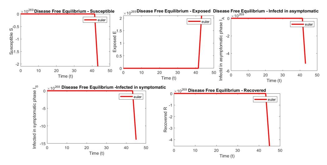
Figure 6: Euler divergence with DF points at h=1.18.
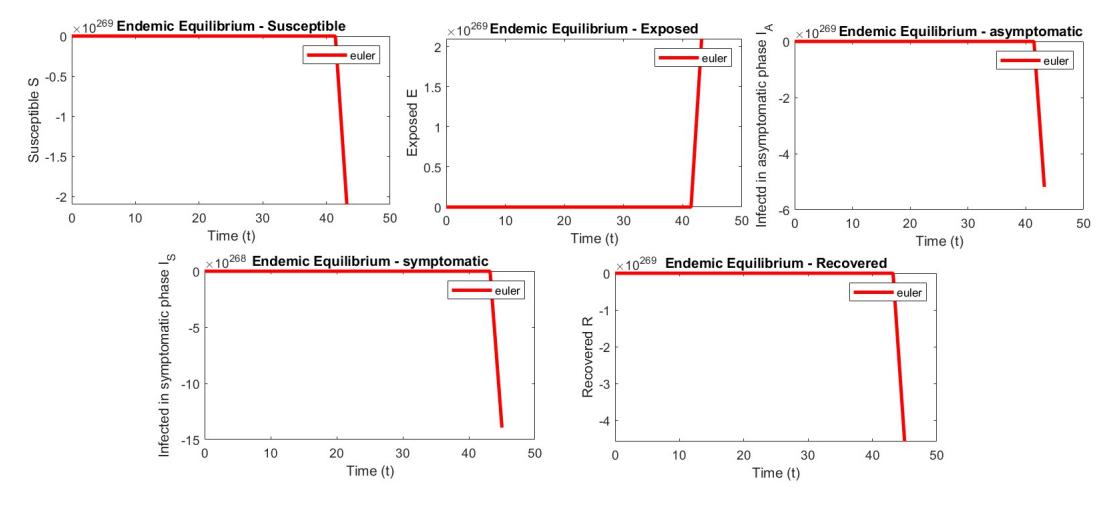
Figure 7: Euler divergence with EE points at h=1.18.
Case 1(b):- NSFD Method Convergence at DF and EE Points
Then, the positive preserving method NSFD method was applied for step size h = 1.18. The method simulation at DF and EE points showed convergent results as shown in Figure 8 and 9. In short, the NSFD method can accurately capture the system's dynamics and to maintain numerical stability and reliability in the solution.
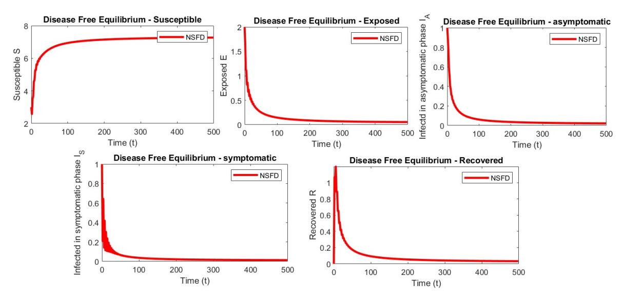
Figure 8: NSFD convergence with DF points at h=1.18.
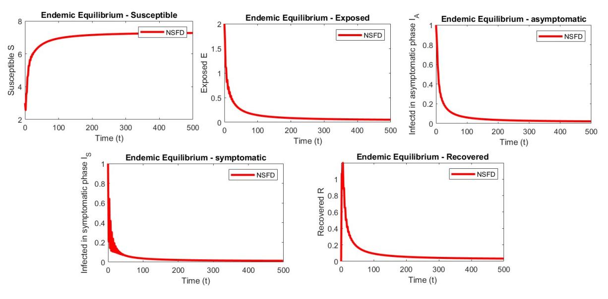
Figure 9: NSFD convergence with EE points at h=1.18.
Case 2(a):- Rk4 method divergence at DF and EE points
Secondly, the Runge–Kutta method was carried out for h = 0.75 for both DF and EE points. Both simulations revealed solutions divergence, as displayed in Figure 10 and 11. Similar with the Euler method, RK4 also fails to accurately capture the system's dynamics and maintain numerical stability and reliability in the solution.
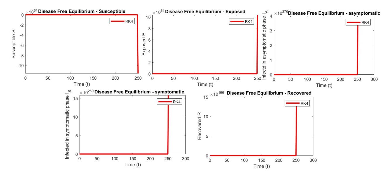
Figure 10: RK4 divergence with DF points at h=0.75.
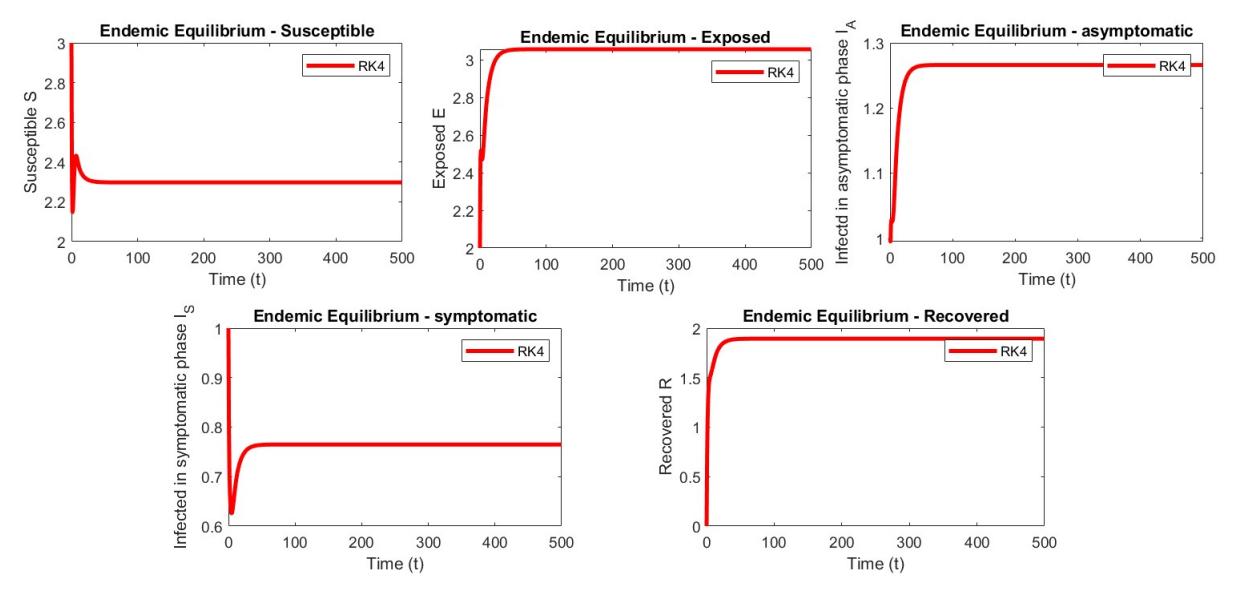
Figure 11: RK4 divergence with EE points at h=0.75.
Case 2(b):- NSFD method convergence at DF and EE points
Then, the proposed positive preserving method NSFD scheme was applied for the solution of this unique model, where h = 0.75. Convergent solutions were obtained both at DF and EE points, as presented by Figure 12 and 13.
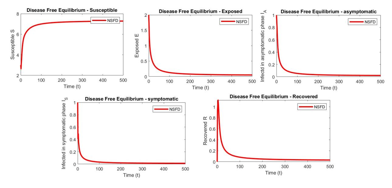
Figure 12: NSFD convergence with DF points at h=0.75.
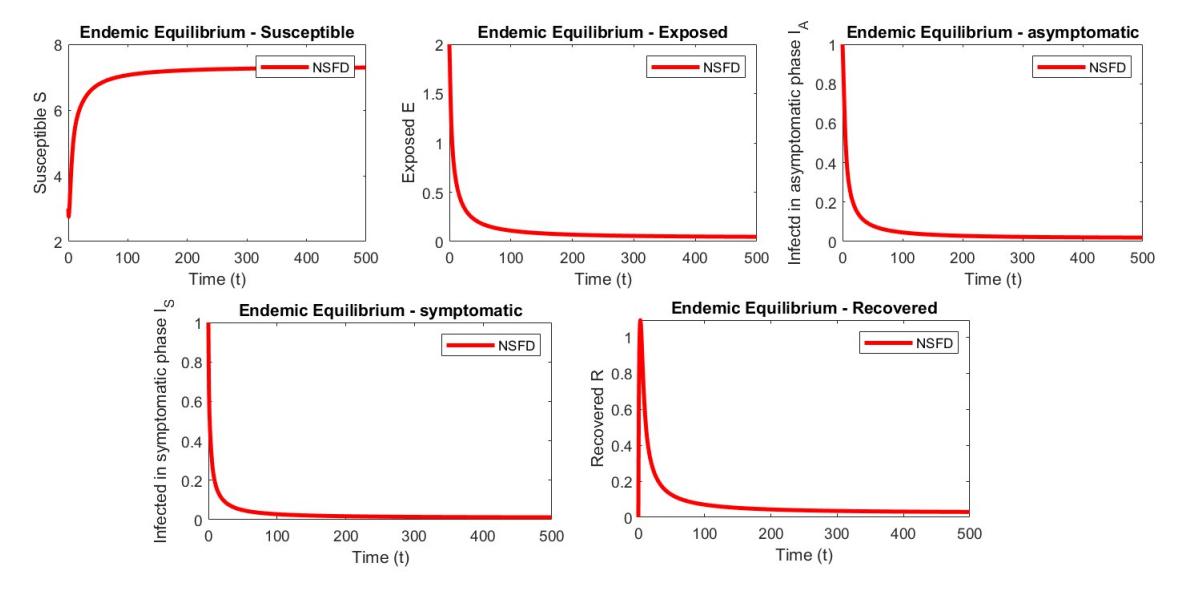
Figure 13: NSFD convergence with EE points at h=0.75.
Case 3:- Effect of large step size on NSFD and time delay behavior
The findings of Case 1 and Case 2 indicate that the Euler and RK-4 schemes did not give accurate and reliable results even at a minimal step size, that is, h = 0.75 and 1.18. However, the proposed NSFD method generated a convergent solution even at significant step sizes as illustrated in Figure14.
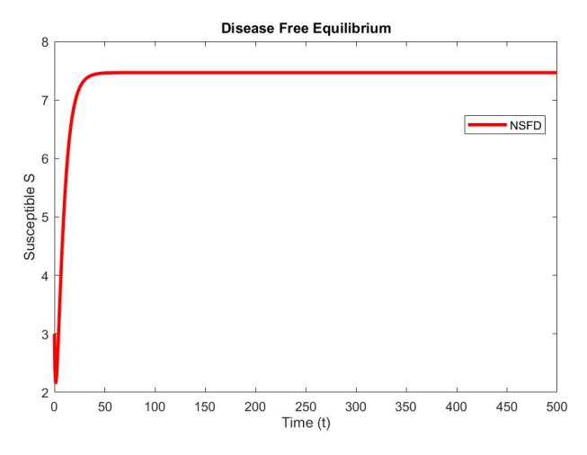
Figure 14: At h=1.5 susceptible compartment by using NSFD method.
From the graphical analysis, it can be concluded that the proposed model can predict future outcomes at very small and large points using NSFD method. Using the same method, increasing the delay rate will decrease the R0, hence disease also decrease in susceptible population. This behavior can be observed in Figure 15 and 16.
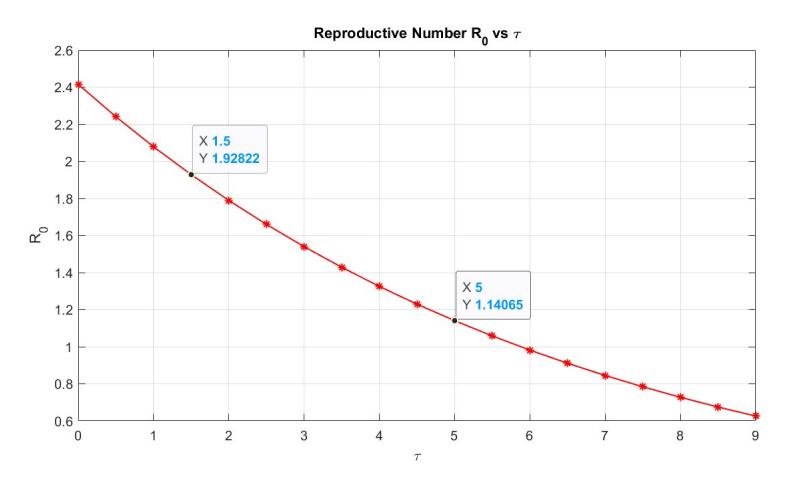
Figure 15: value of R0 that decreases with rising delay ratio τ .
The Euler and RK4 methods produced divergent solutions at small step sizes due to the explicit nature of these methods [57], [58], [59], [60], which can accumulate errors in stiff or nonlinear systems. In contrast, the NSFD method is designed to preserve the qualitative properties of the system, such as positivity and
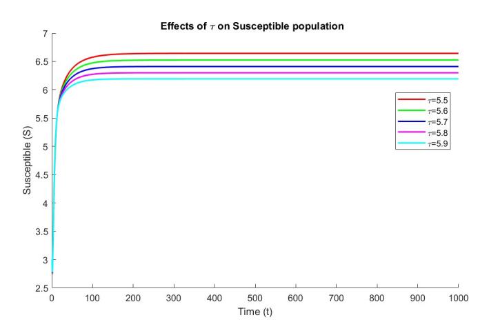
Figure 16: behavior of Susceptible Population with different values of τ .
boundedness, leading to convergent solutions even with small step sizes. This makes NSFD more suitable for handling complex epidemiological models, ensuring numerical stability.
7. CONCLUSION
In this study, a comprehensive mathematical model was developed by extension of simple model to better understand the transmission dynamics of Chlamydia trachomatis, incorporating a biologically relevant time delay to account for the latency period between exposure and infectiousness in susceptible individuals. This exponential time delay reflects the incubation phase during which individuals are infected but not yet infectious, an important epidemiological feature often overlooked in simpler compartmental models. The model accurately captured the unique characteristics of Chlamydia progression by distinguishing between asymptomatic and symptomatic infectious stages, which is critical since a large proportion of Chlamydia infections remain asymptomatic and may go undetected while still contributing to disease transmission. This distinction enhances the model's realism and makes it highly applicable to real-world public health scenarios where symptom-based surveillance is limited. The analytical investigation included the derivation of the basic reproduction number, denoted by R0, which serves as a key threshold parameter indicating whether the infection will die out or become endemic within the population. Through rigorous mathematical analysis, both local and global stability conditions were established for the DF) and EE, offering insight into the longterm behavior of the disease under various epidemiological and intervention-related parameters. The analysis identified parameter regions where Chlamydia can be completely eradicated from the population, as well as scenarios where it persists indefinitely, thus informing time delay control strategies. Moreover, existence and uniqueness theorems were proved to ensure that the model is mathematically well-posed meaning it yields a unique, biologically feasible solution that depends continuously on initial conditions. This provides a solid theoretical foundation for both analytical and numerical explorations.
To numerically solve the system, the NSFD method was employed. This method was carefully constructed to preserve essential qualitative features of the continuous model, including positivity of solutions (ensuring population sizes remain non-negative), boundedness, and consistency with the underlying biological assumptions. Compared to classical numerical schemes such as the explicit Euler method and the RK-4 method, the NSFD approach demonstrated superior performance, particularly in handling stiff dynamics and maintaining stability at smaller time step sizes. This makes it especially suitable for simulating complex epidemic models involving nonlinear interactions and time delays, reinforcing its value as a computational tool in epidemiological modeling and policy planning. A key component of this study was the sensitivity analysis of R0 with respect to critical parameters. It revealed that the transmission rates from asymptomatic and symptomatic individuals (β1 and β2), the fraction of asymptomatic individuals ρ, the progression rate to infectivity η, the natural death rate µ, and the time delay τ significantly influence the disease spread.
These findings provide concrete insights for public health interventions like awareness campaigns, increased condom usage, and routine screening can minimize the probability of transmission during both asymptomatic and symptomatic phases. Since asymptomatic individuals significantly contribute to R0, enhancing screening coverage, especially among high-risk groups, is essential for early detection and treatment. Interventions such as early medical consultation and prophylactic treatments could extend the incubation period and slow down the onset of infectivity. Though not a direct control strategy, understanding its influence helps to refine longterm epidemiological projections, especially in demographically diverse regions. These findings demonstrate that our model provides a more realistic representation of Chlamydia transmission and serves as a powerful analytical tool for assessing intervention strategies. The model's structure allows for flexible integration of control measures like condom use, regular screening, partner limitation, and maintaining a healthy vaginal microbiome, making it particularly valuable for scenario-based simulations and public health planning. Therefore, this work contributes both theoretically and practically to the understanding and management of Chlamydia all over the world. Overall, the model illustrates that a combination of early diagnosis, timely treatment, public awareness, and targeted testing of asymptomatic individuals can greatly reduce the basic reproduction number R0 and thus control the spread of Chlamydia. Future research directions include the development of stochastic and fractional-order versions of the current model to incorporate uncertainty and memory effects. Moreover, fuzzy logic approaches may enhance decision-making under vague parameter estimates. These enhancements will further solidify the model's applicability to complex real-world scenarios.
ACKNOWLEDGEMENT
We gratefully acknowledge the financial support provided by Universiti Sains Malaysia (Main Campus) and the Malaysian International Scholarship.
USE OF AI TOOLS DECLARATION AND DATA AVAILABILITY
The authors declare that no Artificial Intelligence (AI) tools were used in the creation of this article. However, ChatGPT and QuillBot were employed solely for language rephrasing. All data supporting this study are included within the article.
CONFLICT OF INTEREST
The authors confirm that they have no conflicts of interest.