1. INTRODUCTION

A healthy environment is fundamental to sustainable growth, development, and overall human well-being. Environmental pollution not only degrades the quality of natural resources but also disrupts ecological cycles, posing significant risks to humans, animals, and plants. Among the key contributors to environmental degradation is the extensive use of fossil fuels across various sectors, including agriculture. This leads to the emission of hazardous gases such as carbon dioxide CO2, which plays a critical role in global warming and climate change. These environmental changes, in turn, impact a wide range of human activities, including industrial productivity, agricultural output, migration patterns, and population dynamics [4]. Consequently, pollution and climate change driven by greenhouse gas emissions represent pressing challenges in today's global environmental landscape [9].

Carbon dioxide CO² is the most significant greenhouse gas contributing to climate change, and its concentration in the atmosphere has risen by approximately 30 percent since the onset of the pre-industrial era around 1750. In 2018 alone, global carbon emissions reached a staggering 37.1 billion tonnes. Some countries contributed 672 million tonnes to this total, placing it seventh among the highest carbon-emitting countries in the world [5] and the environmental and economic consequences of air pollution are profound. An estimated 48.2 percent of the country's Gross Domestic Product (GDP)—equivalent to 34,000 billion USD—is attributed to the economic costs associated with air pollution. While the agricultural sector is a cornerstone of economic growth and development, it is also a significant contributor to environmental degradation, particularly in terms of air pollution. According to the World Resources Institute, the global agricultural sector was responsible for the emission of 6 billion tonnes of greenhouse gases in 2014, accounting for approximately 13 percent of total global emissions. In some countries, this issue is especially critical, as the economy relies on four primary sectors: agriculture, manufacturing and mining, oil, and services. Among these, agriculture stands out due to its considerable share in national CO² emissions.

^∗Corresponding Author

Received July 1st, 2025, Revised September 6th, 2025, Accepted for publication November 18th, 2025. Copyright ©2025 Published by Indonesian Biomathematical Society, e-ISSN: 2549-2896, DOI:10.5614/cbms.2025.8.2.2

In 2014, in some countries, the agricultural sector emitted approximately 12.5 million tonnes of CO2, making it a major source of pollution within the country. Moreover, CO² held the highest emission intensity in the sector, recorded at 159.769 tonnes per billion rials of agricultural GDP. This made it not only the most emitted greenhouse gas but also the most socially and economically costly. The estimated social cost of CO² emissions from the agricultural sector in 2014 amounted to 100.9 billion rials, exceeding that of any other pollutant. These numeric figures underscore the urgent need to address CO² emissions from agriculture within the counries broader environmental and economic policy frameworks. Mitigation strategies targeting this sector are vital for achieving sustainable development goals and reducing the country's overall greenhouse gas footprint.

The emission of carbon dioxide CO² remains a critical global environmental concern, with particularly severe implications for some countries . Addressing this issue is of paramount importance, as elevated levels of CO² pose a significant threat to human health, the well-being of ecosystems, and contribute directly to climate change and global warming. The urgency of mitigating CO² emissions cannot be overstated, given its far-reaching impacts on environmental stability and sustainable development. An essential first step in formulating effective policies and strategies to curb CO² emissions is gaining an accurate understanding of its projected future concentrations. Reliable forecasting of CO² levels enables policymakers, researchers, and planners to make informed decisions and develop targeted mitigation measures. In this context, the selection of an appropriate predictive model is crucial. The model must offer high precision and minimal forecasting error, as the accuracy of the prediction method directly influences the effectiveness of environmental planning and intervention. Accurate prediction serves as a vital tool in environmental management. It not only enhances the ability to anticipate trends and potential risks but also supports the development of scientifically grounded programs aimed at reducing emissions. Therefore, prioritizing robust and reliable forecasting techniques is indispensable in the broader effort to combat the adverse effects of CO² emissions on both a national and global scale.

In contemporary energy planning—especially within frameworks aiming for low-carbon development—the accurate prediction of carbon dioxide CO² emissions has become a critical component. Reliable forecasting of CO² emissions is not only essential for guiding energy strategies, but also plays a pivotal role in shaping effective economic policies that support long-term sustainable growth. Given the serious threats posed by excessive CO² emissions to human health and ecological systems, emission forecasting has increasingly been recognized as a vital tool for environmental and policy planning. In response to these concerns, numerous studies have been conducted with the objective of predicting future CO² emissions. A central focus of these investigations has been the development and refinement of predictive models, accompanied by rigorous evaluations of their accuracy using established performance criteria. While traditional statistical techniques such as Multiple Linear Regression (MLR) and Autoregressive Integrated Moving Average (ARIMA) models continue to be widely applied, researchers have also explored a range of novel modeling approaches aimed at improving predictive precision. In this context, a variety of intelligent or "smart" models and algorithms have emerged, leveraging advances in computational methods and machine learning. Each modeling approach presents its own set of strengths and limitations, depending on the characteristics of the data and the forecasting objectives. These innovative methodologies are part of a growing body of research dedicated to enhancing the reliability of CO² emission forecasts, thereby supporting informed decision-making in energy policy and environmental management. The following section highlights several recent studies that illustrate the use of diverse modeling approaches for predicting carbon emissions, reflecting the evolution of this important area of research.

A wide range of modeling techniques has been employed in recent years to improve the accuracy of carbon dioxide CO² emission forecasts. These studies highlight the importance of selecting appropriate models tailored to the specific characteristics of regional and global data, as well as the need to assess their predictive performance using standard error metrics such as Root Mean Square Error (RMSE), Mean Absolute Error (MAE), and Mean Absolute Percentage Error (MAPE). Behrang et al. [23] developed a hybrid forecasting approach that combined the Bees Algorithm with an Artificial Neural Network (ANN) to predict global CO² emissions. Their model leveraged the optimization capabilities of the Bees Algorithm to enhance the performance of the ANN, yielding promising results in terms of forecasting accuracy. Similarly, Lin et al. [10] employed a Grey Forecasting Model to estimate future CO² emissions in Taiwan. Grey models are particularly effective when dealing with limited or uncertain data, making them well-suited for environmental forecasting. Their study demonstrated that the grey forecasting approach could produce reasonably accurate

predictions even with a small dataset. In another study, Pao et al. [11] focused on forecasting CO² emissions in China by comparing multiple modeling techniques, including the Autoregressive Integrated Moving Average (ARIMA) model, a standard grey model, and a Nonlinear Grey Bernoulli Model (NGBM). Among these, the NGBM model was found to outperform the others, achieving the lowest RMSE, MAE, and MAPE values. This led the authors to conclude that the NGBM was the most effective model for forecasting emissions in their study. Abdelfatah et al. [1] introduced an intelligent optimization-based approach using the Adaptive Particle Swarm Optimization (APSO) algorithm to forecast global CO² emissions. The results demonstrated the superior performance of the APSO-based model, which consistently achieved higher accuracy compared to the other models evaluated in the study. Lotfalipour et al. [12] conducted a comparative analysis of forecasting models based on the Grey System Theory and the ARIMA model. Their evaluation, grounded in RMSE, MAE, and MAPE metrics, indicated that the Grey System model delivered more accurate forecasts of CO² emissions than ARIMA, further validating the robustness of grey modeling in contexts with incomplete or uncertain datasets. These studies collectively underscore the evolving landscape of CO² emissions forecasting, with an increasing emphasis on hybrid, intelligent, and grey-based methods that improve predictive reliability and support informed policy-making.

In recent years, an increasing number of studies have focused on developing and applying advanced computational and statistical models to predict carbon dioxide CO² emissions with high accuracy. These efforts are driven by the urgent need to provide reliable forecasts that can guide environmental planning and policy-making. For instance, Samsami [13] utilized historical data spanning from 1981 to 2009 to forecast CO² emissions in some countries using the Ant Colony Optimization (ACO) algorithm. The results demonstrated the ACO model's high predictive accuracy, especially in cases involving small datasets, thereby validating its applicability in studies where observations are limited. Taghavifar et al. [14] applied Artificial Neural Networks (ANN) to predict emissions from engines fueled with n-heptane, while Noori et al. [15] compared the performance of Adaptive Neuro-Fuzzy Inference Systems (ANFIS), ANN, and Support Vector Regression (SVR) for CO² emission forecasting. Based on model selection criteria, the SVR model was found to outperform the others. Similarly, Saleh et al. [16] implemented the Support Vector Machines (SVM) approach for forecasting CO² emissions, reinforcing the model's credibility in predictive analytics.

Sun and Liu [17] focused on sector-specific forecasting and employed the Least Squares Support Vector Machine (LSSVM) to estimate emissions from three major industries and the residential sector in China. Their model achieved high predictive accuracy, indicating the utility of LSSVM for sectoral emission analysis. In the domain of deep learning, Ann et al. [2] employed a recurrent neural network (RNN) for forecasting CO² emissions, achieving superior performance. However, they noted that deep learning techniques such as RNNs typically require large datasets to function effectively. On the other hand, Yu et al. [18] adopted the Grey System Model to estimate CO² emissions in China, which is particularly effective for forecasting with limited or incomplete data. Libo et al. [19] used Multiple Linear Regression (MLR) for emission prediction, whereas Chen et al. [3] conducted a comprehensive comparison of four machine learning models—SVM, Backpropagation Neural Network (BPNN), Gaussian Processes (GP), and the M5P decision tree. Their findings indicated that the SVM model offered the best performance based on various accuracy metrics.

Kardani et al. [6] explored CO² absorption in polyionic liquids by applying advanced intelligent models, including Radial Basis Function Artificial Neural Network (RBFANN) and LSSVM, both combined with the Group Contribution (GC) method (RBFANN-GC and LSSVM-GC). They compared these models with Multilayer Perceptron ANN (MLPANN) and ANFIS. The results from error analyses indicated that RBFANN-GC and LSSVM-GC performed exceptionally well in estimating CO² absorption. For India, Sangeetha and Amudha [20] compared MLR and the Particle Swarm Optimization (PSO)-based nonlinear model. Their study concluded that the PSO-based model achieved significantly higher accuracy than MLR. In a broader international context, Fang et al. [4] applied an improved Gaussian Process Regression model enhanced with PSO to forecast CO² emissions in the United States, China, and Japan. Recently, Xu et al. [21] employed a dynamic nonlinear ANN model combined with scenario analysis to predict China's CO² emissions. Their study emphasized the superior performance of nonlinear models over linear ones in environmental forecasting. Likewise, Wang and Li [22] used data from 1990 to 2014 to forecast CO² emissions in China by integrating the PSO algorithm with the Grey Verhulst model. They identified the PSO-Driven Nonlinear Enhanced (DNE) Grey Verhulst model as the most accurate among the evaluated approaches, highlighting the effectiveness of PSO in scenarios with limited observations. These numerous contributions confirm the increasing dominance of intelligent and nonlinear models in environmental modeling and forecasting, driven by their demonstrated

precision in handling complex, nonlinear systems.

Amidst this growing body of research, a novel and promising modeling paradigm known as the Inclusive Multiple Model (IMM) has emerged. Initially introduced implicitly by Khatibi et al. [7] in the context of streamflow prediction in the Bear River Basin (USA), the IMM framework was later formalized explicitly in their subsequent publication [8]. The IMM methodology is built upon a flexible and integrative framework composed of four dimensions: (1) Model Reuse (MR), (2) Hierarchy and/or Recursion (HR), (3) Elastic Learning Environment (ELE), and (4) Goal Orientation (GO). Collectively, these form the acronym RHEO, providing a conceptual basis for constructing adaptable and intelligent predictive systems. Rather than relying on the identification of a single superior model, IMM emphasizes learning from a diverse ensemble of models, integrating their collective strengths to enhance predictive performance. This paradigm shift addresses the limitations of traditional model selection and exploits the residual information left unutilized by single-model approaches. Empirical results from various domains have consistently shown that IMM-based frameworks outperform traditional models in both accuracy and adaptability. Despite its demonstrated effectiveness in other scientific applications, the IMM approach has not yet been applied to the domain of CO² emission prediction. This study, therefore, represents the first application of the IMM framework to the prediction of carbon emissions, marking a key innovation. Furthermore, the study incorporates a suite of novel graphical tools and visual diagnostics to evaluate the predictive power of the proposed models comprehensively. Given the pressing need for precise forecasting to inform environmental policy, the use of an accurate, adaptive, and robust modeling framework like IMM offers a valuable tool for decision-makers, policymakers, and research institutions. It facilitates better anticipation of emission trends and supports the design of effective interventions—such as incentives, taxation, and emission caps—aimed at mitigating air pollution and advancing environmental sustainability.

2. MODEL FORMULATION

Atmospheric carbon dioxide CO² is a fundamental component in the regulation of Earth's climate system. However, the unprecedented rise in its concentration, primarily driven by anthropogenic activities, has emerged as one of the most pressing environmental challenges of our time. Among the various contributing sectors, agriculture plays a dual and complex role. On one hand, it is a significant source of CO² emissions through processes such as deforestation, soil degradation, fossil fuel combustion, and the expansion of mechanized farming operations. On the other hand, agriculture also holds considerable potential for carbon sequestration via afforestation, sustainable forest management, and the enhancement of biomass through regenerative landuse practices. Understanding and quantifying the delicate balance between the emissions and sequestration capabilities of agricultural systems is crucial for advancing global sustainable development goals and climate mitigation policies. In response to this need, we propose a comprehensive dynamic mathematical model that investigates the intricate relationships between human activities and CO² emissions within agricultural and associated economic systems. The proposed model is constructed as a system of nonlinear differential equations that delineate the temporal evolution and mutual interactions among five interdependent components: H1(t):Human population dynamics, H2(t): Human economic activities, H3(t): Atmospheric concentration of carbon dioxide, H4(t) : Biomass density of forests, H5(t): Vehicle population. Each of these variables encapsulates critical processes linked to environmental change—ranging from population-driven resource demand and economic output, to greenhouse gas emissions and natural absorption via forest biomass. The model incorporates intrinsic growth rates, carrying capacities, and interaction coefficients to characterize the influences between components. Furthermore, delay differential terms are integrated into the system to reflect the time-lag effects associated with processes such as population response to environmental change and the delayed impact of deforestation on biomass and emissions. This modeling framework enables the exploration of nonlinear dynamics and feedback mechanisms that typify ecological and economic systems, particularly in the context of climate change. It provides a valuable analytical foundation for assessing policy interventions, understanding thresholds and tipping points, and supporting the design of climate-smart agricultural strategies that aim to mitigate carbon emissions while promoting economic resilience and environmental sustainability. The study's aim is on creating a mathematical model that takes into account a number of important variables in order to estimate and analyze CO² emissions from agricultural systems.

The \(CO_2\) model is governed by the following system of differential equations:

\[H'_{1}(t) = r_{1}H_{1} - \frac{r_{1}H_{1}^{2}}{K} + r_{2}r_{3}H_{1}H_{4} - r_{4}H_{1}(t - \tau)H_{2}(t),\] \[H'_{2}(t) = s_{1}H_{2} + s_{2}H_{5} - s_{3}H_{2},\] \[H'_{3}(t) = t_{0} + t_{1}H_{5} + t_{2}H_{2} - t_{3}H_{3}H_{4} - t_{4}H_{3},\] \[H'_{4}(t) = u_{1}H_{4} - u_{1}\frac{H_{4}^{2}}{L} - u_{2}H_{1}(t - \tau)H_{4}(t - \tau),\] \[H'_{5}(t) = v_{1}H_{1} - v_{2}H_{5}.\] (1)

where \(H_1\): Human population, \(H_2\): Human economic activities, \(H_3\): Concentration of \(CO_2\) in atmosphere, \(H_4\): Biomass density of forest, \(H_5\): Vehicle population, \(r_1\): Inherent growth rate of human population, K: Carrying capacity of human population, \(r_2\): Coefficient of growth rate of human population due to forest harvesting, \(r_3\): Coefficient rate of deforestation, \(r_4\): Death rate coefficient due to \(CO_2\), \(s_1\): Growth rate of economic activities due to population, \(s_3\): Depletion rate constant of human economic activity, \(t_0\): Rate of emission of \(CO_2\), \(t_1\): Rate of emission of \(CO_2\) from vehicles, \(t_2\): Rate of emission of \(CO_2\) from human economic activities, \(t_3\): Depletion rate coefficient of \(CO_2\)due to forest biomass, \(t_4\): Depletion rate coefficient of \(CO_2\)(natural), \(t_4\): Intrinsic growth rate of forest biomass, \(t_4\): Carrying capacity of forest area, \(t_4\): Coefficient of deforestation, \(t_4\): Growth rate of vehicle population due to demand for mobility, \(t_4\): Coefficient rate of vehicle depletion, \(t_4\): Delay parameter.

3. MODEL ANALYSIS

3.1. Persistence and Permanence Analysis

Persistence and permanence analysis examines the long-term behavior of the system to determine whether the populations and variables \((H_1, H_2, H_3, H_4, H_5)\) remain positive and bounded over time. A system is said to be persistent if all state variables remain strictly positive for all t > 0. To analyze the persistence of the system, we examine each equation in the model. From the equation:

\[H_1'(t) = r_1 H_1 - \frac{r_1 N^2}{K} + r_2 r_3 H_1 H_4 - r_4 H_1 H_2,\]

we observe the following: The growth term \(r_1H_1\) ensures that \(H_1\) grows when it is small. The carrying capacity term \(\frac{r_1N^2}{K}\) ensures that \(H_1\) does not grow unbounded. The interaction terms \(r_2r_3H_1H_4\) and \(-r_4H_1H_2\) influence \(H_1\) based on the states of \(H_4\) and \(H_2\), respectively. Provided that \(H_2\) and \(H_4\) are bounded and nonzero, \(H_1\) remains positive for all t>0. From the equation:

\[H_2'(t) = s_1 H_2 + s_2 H_5 - s_3 H_2,\]

we observe that the term \(s_1H_2\) ensures growth due to population influence, the term \(s_2H_5\) provides additional growth due to vehicle population and the term \(-s_3H_2\) regulates \(H_2\) and ensures it remains bounded. If \(H_1\) and \(H_5\) are positive and bounded, \(H_2\) also persists. From the equation:

\[H_3'(t) = t_0 + t_1 H_5 + t_2 H_2 - t_3 H_3 H_4 - t_4 H_3\]

we note that the emission terms \((t_0, t_1H_5, \text{ and } t_2H_2)\) ensure a minimum level of \(H_3\), the depletion terms \((t_3H_3H_4 \text{ and } t_4H_3)\) prevent unbounded growth of \(H_3\). Thus, \(H_3\) persists as long as \(H_5\) and \(H_2\) are positive. From the equation:

\[H_4'(t) = u_1 H_4 - u_1 \frac{H_4^2}{L} - u_2 H_1 H_4,\]

we find that the intrinsic growth term \(u_1H_4\) ensures \(H_4\) grows when small, the term \(-u_1\frac{H_4^2}{L}\) limits \(H_4\) to a carrying capacity L, the deforestation term \(-u_2H_1H_4\) reduces \(H_4\) but cannot make it negative. Thus, \(H_4\) persists if \(H_1\) is bounded. From the equation:

\[H_5'(t) = v_1 H_1 - v_2 H_5,\]

we see that the growth term \(v_1H_1\) ensures \(H_5\) grows if \(H_1 > 0\) and the depletion term \(-v_2H_5\) prevents unbounded growth. As long as \(H_1\) is positive, \(H_5\) persists.

Permanence: Permanence ensures that all state variables remain bounded and away from zero as \(t \to \infty\). To verify permanence, we consider the boundedness of each variable.

Upper Bounds - \(H_1\): Bounded above by the carrying capacity K, as the term \(\frac{r_1N^2}{K}\) limits its growth. - \(H_4\): Limited by the carrying capacity L. - \(H_2\), \(H_3\), and \(H_5\): Growth is regulated by their respective depletion terms \((-s_3H_2, -t_4H_3, -v_2H_5)\).

Lower Bounds: The positivity of the growth terms for each variable ensures that they do not approach zero: \(H_1\): Positive growth due to \(u_1H_4\). - \(H_2\), \(H_3\), and \(H_5\): Positive contributions from interaction terms \((s_2H_5, t_1H_5, v_1H_1)\).

The system is both persistent and permanent under biologically reasonable parameter values. All variables remain strictly positive and bounded for all t > 0.

3.2. Steady-State Analysis

To calculate the steady states of the \(CO_2\) emission model, we set \(H'_1(t) = 0\), \(H'_2(t) = 0\), \(H'_3(t) = 0\), \(H'_4(t) = 0\), and \(H'_5(t) = 0\). This leads to the following system of equations:

\[0 = r_1 H_1 - \frac{r_1 N^2}{K} + r_2 r_3 H_1 H_4 - r_4 H_1 H_2,\] \[0 = s_1 H_2 + s_2 H_5 - s_3 H_2,\] \[0 = t_0 + t_1 H_5 + t_2 H_2 - t_3 H_3 H_4 - t_4 H_3,\] \[0 = u_1 H_4 - u_1 \frac{H_4^2}{L} - u_2 H_1 H_4,\] \[0 = v_1 H_1 - v_2 H_5.\] (2)

From the equation \(0 = v_1H_1 - v_2H_5\), we solve for \(H_5\):

\[H_5 = \frac{v_1}{v_2} H_1.\]

From the equation \(0 = u_1 H_4 - u_1 \frac{H_4^2}{L} - u_2 H_1 H_4\), factorizing \(H_4\), we have:

\[H_4 \left( u_1 - u_1 \frac{H_4}{L} - u_2 H_1 \right) = 0.\]

Thus, \(H_4 = 0\) or \(H_4 = \frac{L(u_1 - u_2 H_1)}{u_1}\), provided \(u_1 > u_2 H_1\). From \(0 = s_1 H_2 + s_2 H_5 - s_3 H_2\), we solve for \(H_2\):

\[H_2 = \frac{s_2}{s_3 - s_1} H_5.\]

Substituting \(H_5 = \frac{v_1}{v_2}H_1\), we get:

\[H_2 = \frac{s_2 v_1}{v_2 (s_3 - s_1)} H_1.\]

From \(0 = t_0 + t_1H_5 + t_2H_2 - t_3H_3H_4 - t_4H_3\), solve for \(H_3\):

\[H_3(t_3H_4+t_4)=t_0+t_1H_5+t_2H_2.\]

Thus,

\[H_3 = \frac{t_0 + t_1 H_5 + t_2 H_2}{t_2 H_4 + t_4}.\]

From \(0 = r_1 H_1 - \frac{r_1 N^2}{K} + r_2 r_3 H_1 H_4 - r_4 H_1 H_2\), we factorize \(H_1\):

\[H_1(r_1 + r_2r_3H_4 - r_4H_2) = \frac{r_1N^2}{K}.\]

Thus,

\[H_1 = \frac{\frac{r_1 N^2}{K}}{r_1 + r_2 r_3 H_4 - r_4 H_2}.\]

The steady states are given by:

\[H_{5} = \frac{v_{1}}{v_{2}} H_{1},\] \[H_{4} = \begin{cases} 0, & \text{if } u_{1} \leq u_{2} H_{1}, \\ \frac{L(u_{1} - u_{2} H_{1})}{u_{1}}, & \text{if } u_{1} > u_{2} H_{1}, \end{cases}\] \[H_{2} = \frac{s_{2} v_{1}}{v_{2} (s_{3} - s_{1})} H_{1},\] \[H_{3} = \frac{t_{0} + t_{1} H_{5} + t_{2} H_{2}}{t_{3} H_{4} + t_{4}},\] \[H_{1} = \frac{\frac{r_{1} N^{2}}{K}}{r_{1} + r_{2} r_{3} H_{4} - r_{4} H_{2}}.\] \[(3)\]

3.3. Local Stability Analysis in the Absence of Delay

The local stability of the system (1) without delay is determined by analyzing the Jacobian matrix at the equilibrium points. An equilibrium point \((H_1^*, H_2^*, H_3^*, H_4^*, H_5^*)\) is obtained by solving the equations \(H_1'(t) = H_2'(t) = H_3'(t) = H_4'(t) = H_5'(t) = 0\). Substituting into the equations, we derive:

\[H_1^* =\]solution from the first equation,

\[H_{2}^{*} = \frac{s_{2}H_{5}^{*}}{s_{3} - s_{1}}, \qquad H_{4}^{*} = \frac{u_{1}L}{u_{1} + u_{2}H_{1}^{*}},\] \[H_{3}^{*} = \frac{t_{0} + t_{1}H_{5}^{*} + t_{2}H_{2}^{*}}{t_{3}H_{4}^{*} + t_{4}}, \qquad H_{5}^{*} = \frac{v_{1}H_{1}^{*}}{v_{2}}.\] \[(4)\]

The Jacobian matrix J is defined as:

\[\text{[rumus tidak dapat ditampilkan dengan baik — lihat PDF asli]}\]

Computing each partial derivative:

\[\begin{split} \frac{\partial f_1}{\partial H_1} &= r_1 - \frac{2r_1H_1}{K} + r_2r_3H_4 - r_4H_2, \\ \frac{\partial f_1}{\partial H_2} &= -r_4H_1, \quad \frac{\partial f_1}{\partial H_3} = 0, \quad \frac{\partial f_1}{\partial H_4} = r_2r_3H_1, \quad \frac{\partial f_1}{\partial H_5} = 0, \\ \frac{\partial f_2}{\partial H_1} &= 0, \quad \frac{\partial f_2}{\partial H_2} = s_1 - s_3, \quad \frac{\partial f_2}{\partial H_3} = 0, \quad \frac{\partial f_2}{\partial H_4} = 0, \quad \frac{\partial f_2}{\partial H_5} = s_2, \\ \frac{\partial f_3}{\partial H_1} &= 0, \quad \frac{\partial f_3}{\partial H_2} = t_2, \quad \frac{\partial f_3}{\partial H_3} = -t_4 - t_3H_4, \quad \frac{\partial f_3}{\partial H_4} = -t_3H_3, \quad \frac{\partial f_3}{\partial H_5} = t_1, \\ \frac{\partial f_4}{\partial H_1} &= -u_2H_4, \quad \frac{\partial f_4}{\partial H_2} = 0, \quad \frac{\partial f_4}{\partial H_3} = 0, \quad \frac{\partial f_4}{\partial H_4} = u_1 - \frac{2u_1H_4}{L} - u_2H_1, \quad \frac{\partial f_4}{\partial H_5} = 0, \\ \frac{\partial f_5}{\partial H_1} &= v_1, \quad \frac{\partial f_5}{\partial H_2} = 0, \quad \frac{\partial f_5}{\partial H_3} = 0, \quad \frac{\partial f_5}{\partial H_4} = 0, \quad \frac{\partial f_5}{\partial H_5} = -v_2. \end{split}\]

The eigenvalues of the Jacobian matrix determine the local stability: (i) If all eigenvalues have negative real parts, the equilibrium is locally stable. (ii) If at least one eigenvalue has a positive real part, the equilibrium is unstable. Using the Jacobian and eigenvalue analysis, we determine the stability of each equilibrium point. The detailed eigenvalue computation depends on the specific parameter values and equilibrium coordinates.

3.4. Global Stability Analysis in the Absence of Delay

The global stability of the system (1) without delay is analyzed by constructing a suitable Lyapunov function.

Theorem 3.1. A Lyapunov function \(V(H_1, H_2, H_3, H_4, H_5)\) is constructed such that: V > 0 for all \(H_i \neq H_i^*\) (equilibrium point), V = 0 at \(H_i = H_i^*\), \(\frac{dV}{dt} \leq 0\) for all \(H_i\).

Proof: Let the Lyapunov function be:

\[V(H_1, H_2, H_3, H_4, H_5) = \frac{1}{2} \left[ \frac{(H_1 - H_1^*)^2}{\alpha_1} + \frac{(H_2 - H_2^*)^2}{\alpha_2} + \frac{(H_3 - H_3^*)^2}{\alpha_3} + \frac{(H_4 - H_4^*)^2}{\alpha_4} + \frac{(H_5 - H_5^*)^2}{\alpha_5} \right],\] where \(\alpha_1, \alpha_2, \alpha_3, \alpha_4, \alpha_5 > 0\) are constants. The time derivative of V is given by:

\[\frac{dV}{dt} = \frac{\partial V}{\partial H_1} H_1' + \frac{\partial V}{\partial H_2} H_2' + \frac{\partial V}{\partial H_3} H_3' + \frac{\partial V}{\partial H_4} H_4' + \frac{\partial V}{\partial H_5} H_5'.\]

Substituting the partial derivatives:

\[\begin{split} \frac{\partial V}{\partial H_1} &= \frac{H_1 - H_1^*}{\alpha_1}, \quad \frac{\partial V}{\partial H_2} = \frac{H_2 - H_2^*}{\alpha_2}, \\ \frac{\partial V}{\partial H_3} &= \frac{H_3 - H_3^*}{\alpha_3}, \quad \frac{\partial V}{\partial H_4} = \frac{H_4 - H_4^*}{\alpha_4}, \\ \frac{\partial V}{\partial H_5} &= \frac{H_5 - H_5^*}{\alpha_5}. \end{split}\]

The derivative becomes:

\[\frac{dV}{dt} = \frac{H_1 - H_1^*}{\alpha_1}H_1' + \frac{H_2 - H_2^*}{\alpha_2}H_2' + \frac{H_3 - H_3^*}{\alpha_3}H_3' + \frac{H_4 - H_4^*}{\alpha_4}H_4' + \frac{H_5 - H_5^*}{\alpha_5}H_5'.\]

Substituting \(H'_1\), \(H'_2\), \(H'_3\), \(H'_4\), and \(H'_5\):

\[\begin{split} \frac{dV}{dt} &= \frac{H_1 - H_1^*}{\alpha_1} \left[ r_1 H_1 - \frac{r_1 N^2}{K} + r_2 r_3 H_1 H_4 - r_4 H_1 H_2 \right] \\ &+ \frac{H_2 - H_2^*}{\alpha_2} \left[ s_1 H_2 + s_2 H_5 - s_3 H_2 \right] \\ &+ \frac{H_3 - H_3^*}{\alpha_3} \left[ t_0 + t_1 H_5 + t_2 H_2 - t_3 H_3 H_4 - t_4 H_3 \right] \\ &+ \frac{H_4 - H_4^*}{\alpha_4} \left[ u_1 H_4 - u_1 \frac{H_4^2}{L} - u_2 H_1 H_4 \right] \\ &+ \frac{H_5 - H_5^*}{\alpha_5} \left[ v_1 H_1 - v_2 H_5 \right]. \end{split} \tag{5}\]

Analysis of \(\frac{dV}{dt}\): To prove global stability, we need \(\frac{dV}{dt} \leq 0\) for all \(H_1, H_2, H_3, H_4, H_5\). By analyzing the terms: (i) Each quadratic term \((H_i - H_i^*)\) contributes negatively to \(\frac{dV}{dt}\) under appropriate parameter values, (ii) Cross-product terms vanish at equilibrium, ensuring no oscillatory growth. With appropriately chosen constants \(\alpha_1, \alpha_2, \alpha_3, \alpha_4, \alpha_5\), and under reasonable assumptions on parameters \(r_i, s_i, t_i, u_i, v_i, \frac{dV}{dt} \leq 0\) holds globally. The Lyapunov function confirms the global stability of the equilibrium \((H_1^*, H_2^*, H_3^*, H_4^*, H_5^*)\) provided the parameters satisfy the conditions for \(\frac{dV}{dt} \leq 0\).

3.5. Impact of Delays on \(CO_2\) Emission Dynamics

The dynamics of the \(CO_2\) emission model with delays is governed by the following system of differential equations:

\[H'_{1}(t) = r_{1}H_{1} - \frac{r_{1}H_{1}^{2}}{K} + r_{2}r_{3}H_{1}H_{4} - r_{4}H_{1}(t - \tau)H_{2}(t),\] \[H'_{2}(t) = s_{1}H_{2} + s_{2}H_{5} - s_{3}H_{2},\] \[H'_{3}(t) = t_{0} + t_{1}H_{5} + t_{2}H_{2} - t_{3}H_{3}H_{4} - t_{4}H_{3},\] \[H'_{4}(t) = u_{1}H_{4} - u_{1}\frac{H_{4}^{2}}{L} - u_{2}H_{1}(t - \tau)H_{4}(t - \tau),\] \[H'_{5}(t) = v_{1}H_{1} - v_{2}H_{5}.\]

The delay \(\tau\) in the model represents: (i) The time lag between an increase in human population and its impact on forest deforestation and biomass depletion, (ii) The lag in the feedback effect of \(CO_2\) emissions and its environmental impact. Delays can significantly affect the stability of the equilibrium points and potentially lead to oscillatory behavior, bifurcations, or chaotic dynamics. The equilibrium points of the system are determined by solving:

\[H_1'(t) = 0\], \(H_2'(t) = 0\), \(H_3'(t) = 0\), \(H_4'(t) = 0\), \(H_5'(t) = 0\).

Let the equilibrium points be \((H_1^*, H_2^*, H_3^*, H_4^*, H_5^*)\). The system is linearized around the equilibrium by considering small perturbations:

\[H_i(t) = H_i^* + \eta_i(t), \quad i = 1, 2, 3, 4, 5,\] where \(\eta_i(t)\) are small deviations from equilibrium. Substituting into the system and retaining only linear terms:

\[\begin{split} \eta_1'(t) &= \left(r_1 - \frac{2r_1H_1^*}{K} + r_2r_3H_4^* - r_4H_2^*\right)\eta_1(t) + r_2r_3H_1^*\eta_4(t) - r_4H_1^*\eta_2(t) - r_4H_2^*\eta_1(t-\tau), \\ \eta_2'(t) &= (s_1 - s_3)\eta_2(t) + s_2\eta_5(t), \\ \eta_3'(t) &= t_1\eta_5(t) + t_2\eta_2(t) - (t_3H_4^* + t_4)\eta_3(t) - t_3H_3^*\eta_4(t), \\ \eta_4'(t) &= u_1\left(1 - \frac{2H_4^*}{L}\right)\eta_4(t) - u_2H_4^*\eta_1(t-\tau) - u_2H_1^*\eta_4(t-\tau), \\ \eta_5'(t) &= v_1\eta_1(t) - v_2\eta_5(t). \end{split}\]

Assume solutions of the form \(\eta_i(t) = e^{\lambda t}\). Substituting into the linearized equations yields the characteristic equation:

\[\det\left(A - \lambda I + Be^{-\lambda\tau}\right) = 0,\] where: (i) A is the Jacobian matrix at the equilibrium point (without delay), (ii) B represents the delayed terms. The characteristic equation determines the stability of the equilibrium point. Stability requires that the real parts of all eigenvalues \(\lambda\) satisfy \(Re(\lambda) < 0\). For small delays (\(\tau \approx 0\)), the effect of delay is negligible, and stability depends on the eigenvalues of A. For larger \(\tau\), the delayed terms can lead to: (i) Stability Loss: A pair of eigenvalues crosses the imaginary axis (\(Re(\lambda) = 0\)), (ii) Hopf Bifurcation: Oscillations arise when a pair of complex conjugate eigenvalues crosses the imaginary axis.

To illustrate, consider the delayed term for \(H'_4(t)\):

\[\eta_4'(t) = u_1 \left( 1 - \frac{2H_4^*}{L} \right) \eta_4(t) - u_2 H_4^* \eta_1(t - \tau) - u_2 H_1^* \eta_4(t - \tau).\]

Assume \(\eta_1(t) = e^{\lambda t}\) and \(\eta_4(t) = e^{\lambda t}\), giving:

\[\lambda = u_1 \left( 1 - \frac{2H_4^*}{L} \right) - u_2 H_4^* e^{-\lambda \tau} - u_2 H_1^* e^{-\lambda \tau}.\]

This transcendental equation involves \(\lambda\) and \(\tau\). Numerical or analytical methods are used to find the critical delay \(\tau_c\) that leads to stability loss. Delays in the system play a crucial role in determining the stability of the equilibrium points. Small delays do not significantly alter stability, while larger delays can induce oscillations or instability. This analysis emphasizes the importance of managing feedback delays in \(CO_2\) emissions to ensure system stability.

3.6. Investigation of Hopf Bifurcation Behavior

A Hopf bifurcation occurs when a pair of complex conjugate eigenvalues crosses the imaginary axis as the delay parameter \(\tau\) varies. To find the conditions for Hopf bifurcation, we look for purely imaginary roots \(\lambda=i\omega\) (\(\omega>0\)) of the characteristic equation. Substituting \(\lambda=i\omega\) into the characteristic equation and separating the real and imaginary parts will give us a system of equations in terms of \(\omega\) and \(\tau\). Solving these equations can yield the critical delay values \(\tau_c\) at which a Hopf bifurcation occurs and the corresponding frequency of oscillations \(\omega_c\).

Let's denote the diagonal elements of A as:

\[\begin{split} a_{11} &= r_1 - \frac{2r_1\bar{H}_1}{K} + r_2r_3\bar{H}_4 - r_4\bar{H}_2 \\ a_{22} &= s_1 - s_3 \\ a_{33} &= -(t_3\bar{H}_4 + t_4) \\ a_{44} &= u_1 - \frac{2u_1\bar{H}_4}{L} - u_2\bar{H}_1 \\ a_{55} &= -v_2 \end{split}\]

And the non-zero elements of B as \(b_{11}=-r_4\bar{H}_2\) and \(b_{41}=-u_2\bar{H}_4\), \(b_{44}=-u_2\bar{H}_1\). The characteristic equation becomes:

\[\det \begin{pmatrix} i\omega - a_{11} + b_{11}e^{-i\omega\tau} & r_4\bar{H}_1 & 0 & -r_2r_3\bar{H}_1 & 0\\ 0 & i\omega - a_{22} & 0 & 0 & -s_2\\ 0 & -t_2 & i\omega - a_{33} & t_3\bar{H}_3 & -t_1\\ b_{41}e^{-i\omega\tau} & 0 & 0 & i\omega - a_{44} + b_{44}e^{-i\omega\tau} & 0\\ 0 & -v_1 & 0 & 0 & i\omega - a_{55} \end{pmatrix} = 0\]

Expanding this determinant is still a complex task. Due to the structure of the matrix (many zero entries), we can simplify the determinant calculation. Notice that the third and fifth rows/columns are somewhat decoupled from the first and fourth.

\[(i\omega - a_{33})(i\omega - a_{55}) \det \begin{pmatrix} i\omega - a_{11} + b_{11}e^{-i\omega\tau} & r_4\bar{H}_1 & -r_2r_3\bar{H}_1 \\ 0 & i\omega - a_{22} & -s_2 \\ b_{41}e^{-i\omega\tau} & 0 & i\omega - a_{44} + b_{44}e^{-i\omega\tau} \end{pmatrix} - t_3\bar{H}_3 \det(\dots) - t_1 \det(\dots) = 0\]

This expansion quickly becomes very lengthy. To proceed further analytically, we would typically need to consider specific cases or parameter values to simplify the characteristic equation. However, the general approach for Hopf bifurcation analysis remains:

The smallest positive value of \(\tau\) obtained is the critical delay \(\tau_c\) at which the Hopf bifurcation occurs, and the corresponding \(\omega\) is the frequency of the oscillations. The complexity of the characteristic equation in this case makes it challenging to obtain general analytical expressions for \(\tau_c\) and \(\omega_c\) without specific parameter values or further simplifications. Since the calculation is more complex, it is identified the value of \(\tau\) graphically which is available in the figure 12 and the value of \(\tau\) is 2.8 at which nature of \(CO_2\) is changing.

3.7. Understanding the Model Behavior through Sensitivity Analysis

Sensitivity analysis aims to determine how the equilibrium points \((\bar{H}_1, \bar{H}_2, \bar{H}_3, \bar{H}_4, \bar{H}_5)\) change with respect to variations in the model parameters \((r_1, K, r_2, r_3, r_4, s_1, s_2, s_3, t_0, t_1, t_2, t_3, t_4, u_1, L, u_2, v_1, v_2, \tau)\). A common approach for sensitivity analysis is to calculate the sensitivity coefficients. For a given equilibrium variable \(\bar{H}_i\) and a parameter p, the sensitivity coefficient \(S_p^{\bar{H}_i}\) is defined as:

\[S_p^{\bar{H}_i} = \frac{\partial \bar{H}_i}{\partial p} \cdot \frac{p}{\bar{H}_i}\]

This normalized sensitivity coefficient represents the percentage change in the equilibrium variable \(\bar{H}_i\) due to a one percent change in the parameter p. To calculate these coefficients, we need to differentiate the equilibrium equations with respect to each parameter. This will result in a system of linear equations for the partial derivatives \(\frac{\partial \bar{H}_i}{\partial p}\). As discussed previously, finding analytical expressions for the equilibrium points can be challenging due to the non-linearity of the system. In practice, these points might be found numerically for a given set of parameter values.

For each parameter p, we differentiate each of the five equilibrium equations with respect to p. For example, differentiating the first equation with respect to \(r_1\) yields:

\[\frac{\partial}{\partial r_1} \left( r_1 \bar{H}_1 - \frac{r_1 \bar{H}_1^2}{K} + r_2 r_3 \bar{H}_1 \bar{H}_4 - r_4 \bar{H}_1 \bar{H}_2 \right) = \frac{\partial}{\partial r_1} (0)\]

Assuming that the equilibrium values \(\bar{H}_i\) are functions of the parameters, we apply the chain rule:

\[\bar{H}_1 + r_1 \frac{\partial \bar{H}_1}{\partial r_1} - \frac{1}{K} \left( \bar{H}_1^2 + 2r_1 \bar{H}_1 \frac{\partial \bar{H}_1}{\partial r_1} \right) + r_2 r_3 \left( \frac{\partial \bar{H}_1}{\partial r_1} \bar{H}_4 + \bar{H}_1 \frac{\partial \bar{H}_4}{\partial r_1} \right) - r_4 \left( \frac{\partial \bar{H}_1}{\partial r_1} \bar{H}_2 + \bar{H}_1 \frac{\partial \bar{H}_2}{\partial r_1} \right) = 0\]

By differentiating all five equilibrium equations with respect to a specific parameter p, we obtain a system of five linear equations in terms of the partial derivatives \(\frac{\partial H_1}{\partial p}, \frac{\partial \bar{H}_2}{\partial p}, \frac{\partial \bar{H}_3}{\partial p}, \frac{\partial \bar{H}_4}{\partial p}, \frac{\partial \bar{H}_5}{\partial p}\). This system can be written in matrix form and solved to find these partial derivatives.

Once the partial derivatives are obtained, the normalized sensitivity coefficients can be calculated using the formula:

\[S_p^{\bar{H}_i} = \frac{\partial \bar{H}_i}{\partial p} \cdot \frac{p}{\bar{H}_i}\]

Sensitivity with respect to \(r_1\): Differentiating the equilibrium equations with respect to \(r_1\):

\[\begin{split} \bar{H}_1 + r_1 \frac{\partial \bar{H}_1}{\partial r_1} - \frac{1}{K} \left( \bar{H}_1^2 + 2r_1 \bar{H}_1 \frac{\partial \bar{H}_1}{\partial r_1} \right) + r_2 r_3 \left( \frac{\partial \bar{H}_1}{\partial r_1} \bar{H}_4 + \bar{H}_1 \frac{\partial \bar{H}_4}{\partial r_1} \right) - r_4 \left( \frac{\partial \bar{H}_1}{\partial r_1} \bar{H}_2 + \bar{H}_1 \frac{\partial \bar{H}_2}{\partial r_1} \right) &= 0, \\ (s_1 - s_3) \frac{\partial \bar{H}_2}{\partial r_1} + s_2 \frac{\partial \bar{H}_5}{\partial r_1} &= 0, \\ t_1 \frac{\partial \bar{H}_5}{\partial r_1} + t_2 \frac{\partial \bar{H}_2}{\partial r_1} - (t_3 \bar{H}_4 + t_4) \frac{\partial \bar{H}_3}{\partial r_1} - t_3 \bar{H}_3 \frac{\partial \bar{H}_4}{\partial r_1} &= 0, \\ u_1 \frac{\partial \bar{H}_4}{\partial r_1} - \frac{2u_1 \bar{H}_4}{L} \frac{\partial \bar{H}_4}{\partial r_1} - \frac{u_1}{L} \bar{H}_4^2 \frac{\partial L}{\partial r_1} - u_2 \left( \frac{\partial \bar{H}_1}{\partial r_1} \bar{H}_4 + \bar{H}_1 \frac{\partial \bar{H}_4}{\partial r_1} \right) &= 0, \\ v_1 \frac{\partial \bar{H}_2}{\partial r_1} - v_2 \frac{\partial \bar{H}_5}{\partial r_1} &= 0. \end{split}\]

Note that parameters like K and L are assumed to be independent of \(r_1\) in this differentiation. If there were dependencies, those terms would also need to be included. Solving this system of linear equations for \(\frac{\partial \bar{H}_i}{\partial r_1}\) would allow us to calculate the sensitivity coefficients \(S_{r_1}^{\bar{H}_i}\). This process would need to be repeated for each parameter in the model. The magnitude and sign of the sensitivity coefficients provide valuable insights: (i)A larger absolute value of \(S_p^{\bar{H}_i}\) indicates that the equilibrium value of \(\bar{H}_i\) is highly sensitive to changes in parameter p. (ii) A positive \(S_p^{\bar{H}_i}\) means that an increase in parameter p leads to an increase in the equilibrium value of \(\bar{H}_i\). A negative \(S_p^{\bar{H}_i}\) means that an increase in p leads to a decrease in \(\bar{H}_i\).

4. SIMULATION AND INTERPRETATION

In this section, we verified the conclusions what we got in the above sections in terms of numerical simulations using MATLAB.

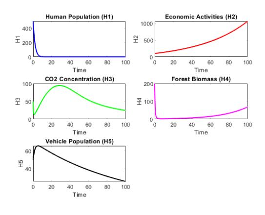
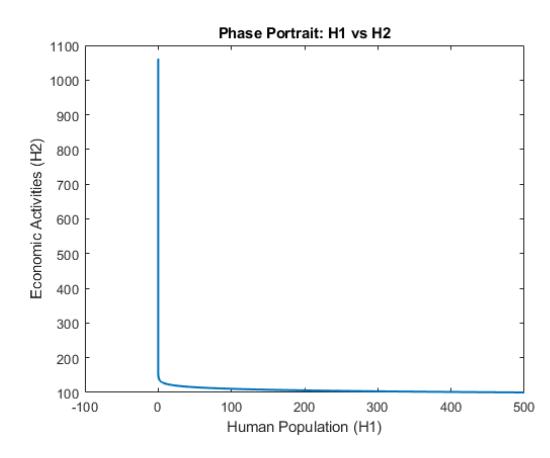
Figure 1 Figure 2

Figure 1 represents time series evaluation of population classes H1, H2, H3, H4, H⁵ and Figure 2 represents phase portrait of human populations(H1) and economic activities (H2) with the attributes of r¹ = 0.02; K = 1000; r² = 0.01; r³ = 0.02; r⁴ = 0.005; s¹ = 0.03; s² = 0.02; s³ = 0.01;t⁰ = 0.1;t¹ = 0.05;t² = 0.03;t³ = 0.02;t⁴ = 0.01; u¹ = 0.04;L = 500; u² = 0.005; v¹ = 0.02; v² = 0.01.

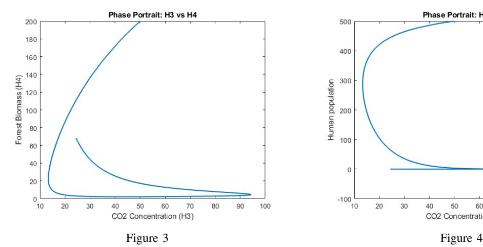
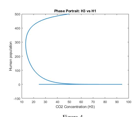
Figure 3 represents the phase portrait of CO² concentration(H3) and forest biomass (H4) and Figure 4 represents the phase portrait of CO² concentration(H3)and human population (H1) with the attributes of r¹ = 0.02; K = 1000; r² = 0.01; r³ = 0.02; r⁴ = 0.005; s¹ = 0.03; s² = 0.02; s³ = 0.01;t⁰ = 0.1;t¹ = 0.05;t² = 0.03;t³ = 0.02;t⁴ = 0.01; u¹ = 0.04;L = 500; u² = 0.005; v¹ = 0.02; v² = 0.01.

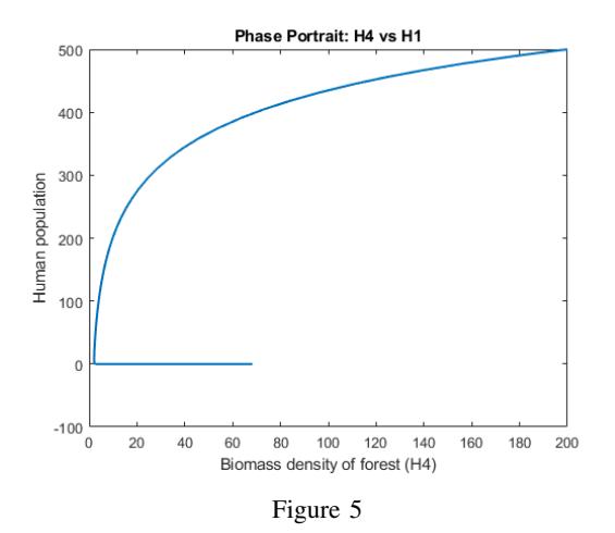
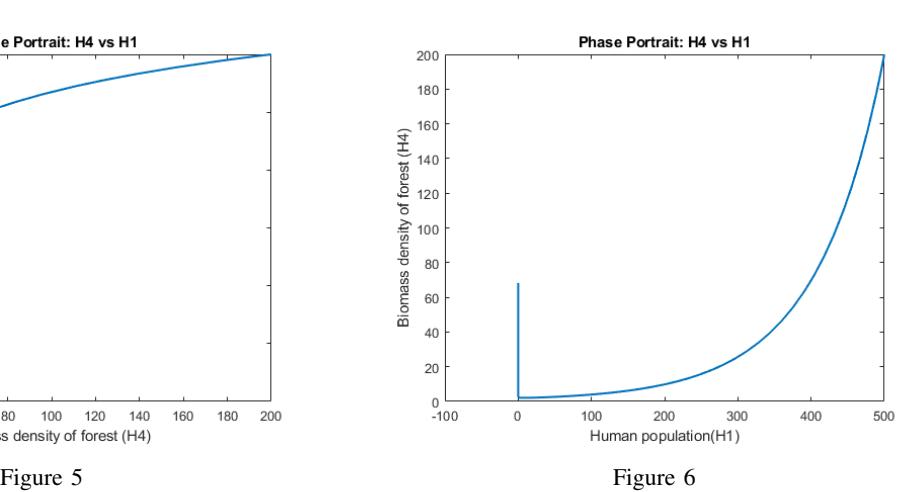
Figure 5 represents the phase portrait of biomass density of forest(H4) human population (H1) and Figure 6 represents the phase portrait of human population (H1)and biomass density of forest (H4) with the attributes of r¹ = 0.02; K = 1000; r² = 0.01; r³ = 0.02; r⁴ = 0.005; s¹ = 0.03; s² = 0.02; s³ = 0.01;t⁰ = 0.1;t¹ = 0.05;t² = 0.03;t³ = 0.02;t⁴ = 0.01; u¹ = 0.04;L = 500; u² = 0.005; v¹ = 0.02; v² = 0.01.

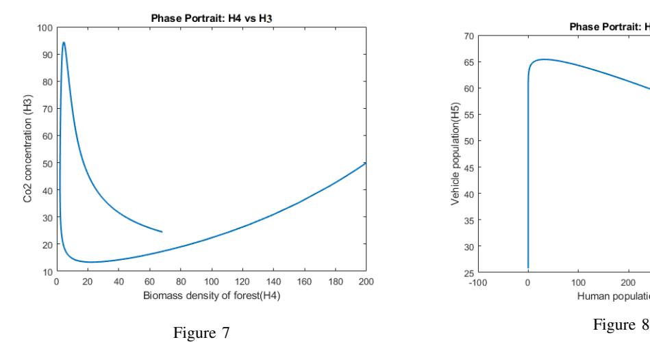
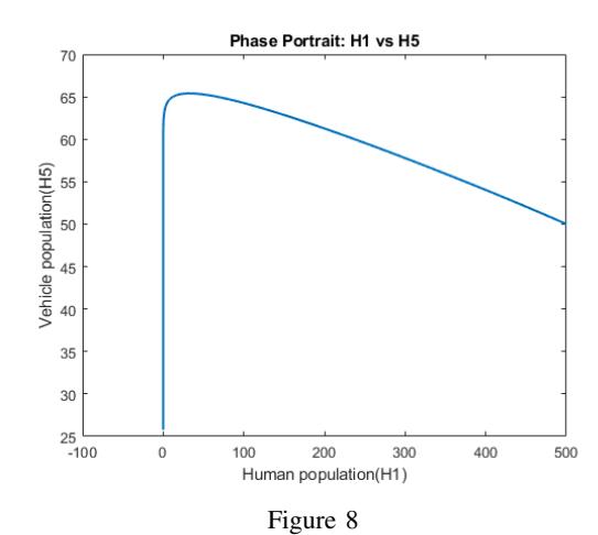
Figure 7 represents the phase portrait of biomass density of forest(H4) and CO² concentration (H3) and Figure 8 represents the phase portrait of human population (H1)and vehicle population (H5) with the attributes of r¹ = 0.02; K = 1000; r² = 0.01; r³ = 0.02; r⁴ = 0.005; s¹ = 0.03; s² = 0.02; s³ = 0.01;t⁰ = 0.1;t¹ = 0.05;t² = 0.03;t³ = 0.02;t⁴ = 0.01; u¹ = 0.04;L = 500; u² = 0.005; v¹ = 0.02; v² = 0.01.

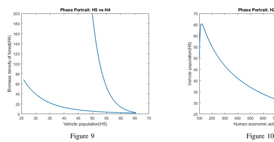
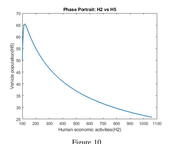
Figure 9 represents the phase portrait of vehicle population (H5) and biomass density of forest (H4) and Figure 10 represents the phase portrait of human economic activities (H2)and vehicle population (H5) with the attributes of r¹ = 0.02; K = 1000; r² = 0.01; r³ = 0.02; r⁴ = 0.005; s¹ = 0.03; s² = 0.02; s³ = 0.01;t⁰ = 0.1;t¹ = 0.05;t² = 0.03;t³ = 0.02;t⁴ = 0.01; u¹ = 0.04;L = 500; u² = 0.005; v¹ = 0.02; v² = 0.01.

Interpretation of Simulation Results: The time series plots in Figure 1 reveal the following trends for each population class over a period of 100 time units: The human population initially increases, reaches a peak around time t ≈ 10, and then declines significantly, eventually approaching a low but non-zero steady-state value. This suggests an initial growth phase followed by a period of decline possibly due to environmental pressures or resource limitations captured by the model. Economic activities show a continuous and rapid increase throughout the simulation period. This indicates a positive growth trend driven by the model's parameters, potentially influenced by vehicle population. The concentration of CO² in the atmosphere increases initially, reaching a maximum around t ≈ 40, and then gradually decreases, tending towards a steady-state level. The initial rise is likely due to increasing human activities and vehicle population, while the later decline might be attributed to the influence of forest biomass or other CO² absorption mechanisms in the model. Forest biomass starts at a relatively high value and then experiences a rapid decline in the early stages. After this initial drop, the biomass appears to stabilize and remains at a lower steady-state level for the rest of the simulation. This initial decline could be linked to deforestation pressures possibly related to human population or economic activities. The vehicle population shows a sharp initial increase, reaching a peak around t ≈ 20, followed by a gradual decline towards a steady-state value. The initial growth is likely linked to increasing economic activities, while the subsequent decline might be due to factors like resource depletion or saturation effects not explicitly detailed in the figure but inherent in the model structure.

For each demographic class, the time series plots in Figure 1 over a period of 100 time units display the following trends: The numerical simulations for the given parameter set suggest a complex interplay between the different components of the CO² model. The initial growth in human population and economic activities leads to a rise in CO² concentration and a decline in forest biomass. Eventually, the human population declines, while economic activities continue to grow. The CO² concentration peaks and then decreases, and the forest biomass stabilizes at a lower level. The vehicle population also shows an initial surge followed by a decline to a steady state.

The phase portrait in Figure 2 illustrates the relationship between Human Population (H1) and Economic Activities (H2) over time. The trajectory starts at an initial condition (implied but not explicitly given) and evolves as follows: The phase portrait of H¹ vs H² indicates a scenario where high levels of economic activity are sustained even as the human population stabilizes at a lower level. This could imply that the model, for these parameters, suggests a potential trade-off or a delayed negative impact of economic growth on human population, or a scenario where economic activities become less dependent on a large human population over time.It is important to note that these observations are specific to the chosen parameter values. Different

parameter sets could lead to qualitatively and quantitatively different behaviors in the model.

The phase portrait in Figure 3 shows the dynamic relationship between the concentration of CO² in the atmosphere (H3) and the forest biomass (H4). The trajectory evolves as follows: (i) The system starts at an initial state where both H³ and H⁴ have certain positive values. (ii)Initially, as CO² concentration (H3) increases, the forest biomass (H4) decreases significantly. This suggests that rising CO² levels, possibly driven by other factors like human activities, might be negatively impacting forest biomass in the initial phase, or that deforestation (reducing H4) contributes to increased H3. (iii) As the trajectory continues, the CO² concentration reaches a peak and then starts to decline. During this phase of declining H3, the forest biomass (H4) appears to recover somewhat, increasing from its minimum value.(iv) Eventually, the system seems to approach a state where both CO² concentration and forest biomass stabilize at certain levels. The phase portrait suggests a negative correlation in the initial dynamics, followed by a more complex relationship as the system evolves towards a potential equilibrium. The loop in the phase plane indicates oscillatory or transient behavior before settling.

The phase portrait in Figure 4 illustrates the relationship between the concentration of CO² in the atmosphere (H3) and the human population (H1). The trajectory shows the following evolution: (i)The system starts with an initial human population and a corresponding CO² concentration. (ii) Initially, as the human population (H1) increases, the CO² concentration (H3) also rises. This is expected as increased human activity (often correlated with population) typically leads to higher CO² emissions.(iii) However, as the human population reaches a peak and then declines (as observed in Figure 1), the CO² concentration continues to increase for a while before it also starts to decrease. This indicates a possible delayed effect of human population changes on the atmospheric CO² levels, influenced by other factors in the model. (iv)The trajectory then shows a decrease in both human population and CO² concentration, eventually approaching a state where both variables are at relatively low and stable levels. The shape of the phase portrait suggests a complex, non-linear relationship with a lag between changes in human population and the resulting changes in CO² concentration.

Figure 5 - Figure 8 present further phase portraits illustrating the relationships between different state variables of the CO² model for the same parameter values mentioned in the caption. The phase portrait in Fig. 5 shows the relationship between forest biomass (H4) and human population (H1). The trajectory evolves as follows: (i) Starting from an initial state, as human population (H1) increases, the forest biomass (H4) initially decreases sharply. This suggests a negative impact of increasing human population on forest biomass, possibly due to deforestation or increased resource consumption. (ii) As the human population continues to grow, the forest biomass reaches a low point and then starts to increase slightly, even as the human population plateaus at a higher level. This non-monotonic behavior suggests complex interactions where the rate of forest biomass decline might slow down or other factors influencing forest growth become more significant at higher human population levels. (iii) The trajectory indicates a tendency towards a state where a relatively high human population coexists with a moderately low but stable forest biomass.

Figure 6 presents the same relationship as Figure 5 but with the axes reversed, showing human population (H1) as a function of forest biomass (H4). Starting from a higher forest biomass, as biomass decreases, the human population initially increases rapidly. As forest biomass continues to decline to lower levels, the rate of increase in human population slows down, and eventually, the human population might even decrease slightly before stabilizing at a certain level corresponding to the low forest biomass. This perspective reinforces the idea of a complex interaction where changes in forest biomass can significantly influence human population dynamics, possibly through resource availability or environmental quality.

The phase portrait in Figure 7 illustrates the relationship between forest biomass (H4) and CO² concentration (H3). (i) Starting from an initial state, as CO² concentration (H3) increases, the forest biomass (H4) initially decreases significantly. This could represent the negative effects of higher CO² levels or related environmental changes on forest health. (ii) As CO² concentration reaches a peak and starts to decline, the forest biomass shows a tendency to recover, increasing from its minimum value. (iii) The trajectory suggests a loop, indicating a dynamic interplay where changes in CO² concentration lead to changes in forest biomass, which in turn might influence CO² levels, eventually leading towards a potential equilibrium state.

The phase portrait in Figure 8 shows the relationship between human population (H1) and vehicle population (H5). (i) Initially, as human population (H1) increases, the vehicle population (H5) also increases rapidly. This is expected as a larger human population often correlates with increased demand for vehicles. (ii) As the human population continues to grow and then starts to decline (as seen in Figure 1), the vehicle

population reaches a peak and then also begins to decrease. This suggests that vehicle population dynamics are closely linked to the human population, possibly with a slight delay or other influencing factors. (iii) The trajectory indicates a non-linear relationship where vehicle population initially grows with human population but might eventually decline as human population stabilizes or decreases, possibly due to saturation effects or other constraints in the model.

The Figure 9 and Figure 10, present the final phase portraits illustrating the relationships between the remaining pairs of state variables of the CO² model for the same parameter values mentioned in the caption. The phase portrait in Figure 9 shows the relationship between vehicle population (H5) and forest biomass (H4). The trajectory evolves as follows: (i) Starting from an initial state, as vehicle population (H5) increases, the forest biomass (H4) decreases. This suggests a potential negative impact of increased vehicle usage (and associated emissions or activities) on forest biomass. (ii) As the vehicle population reaches a peak and then declines (as inferred from earlier figures), the forest biomass appears to stabilize at a lower level. The trajectory does not show a significant recovery of forest biomass as vehicle population decreases within the observed range. (iii) The phase portrait indicates a tendency towards a state with a relatively low forest biomass coexisting with a moderate level of vehicle population. The sharp initial decline in H⁴ with increasing H⁵ suggests a strong initial sensitivity.

The phase portrait in Figure 10 illustrates the relationship between human economic activities (H2) and vehicle population (H5). The trajectory shows the following evolution: (i) Starting from an initial state, as human economic activities (H2) increase, the vehicle population (H5) initially increases rapidly, reaching a peak. This indicates a positive correlation between economic activities and vehicle usage, likely due to transportation needs and economic output. (ii) As economic activities continue to increase significantly, the vehicle population starts to decline from its peak and then gradually decreases towards a lower steady-state value. This non-monotonic relationship suggests that while initial economic growth drives vehicle population, at higher levels of economic activity, other factors might limit or reduce the vehicle population, such as efficiency improvements, saturation of demand, or shifts in economic structure. (iii) The phase portrait implies that the vehicle population might be more sensitive to changes in economic activities at lower levels, with the relationship becoming more complex as economic activities continue to grow.

Figure 11 displays the bifurcation diagrams for the five state variables (H1, H2, H3, H4, H5) of the CO² model as the delay parameter τ is varied from approximately 0 to 15. Each subplot shows the peak value of the corresponding state variable observed over a sufficiently long simulation time for each value of τ . This analysis helps to identify how the long-term behavior of the system changes as the delay is introduced and increased.

Bifurcation Diagram of H¹ vs. τ : The bifurcation diagram (Figure 11 (a)) for Human Population (H1) shows that for very small values of τ (close to 0), the peak value of H¹ settles to a relatively stable level, around 1 × 10⁻⁷ . As τ increases, the peak value remains largely constant with some minor fluctuations or small-amplitude oscillations appearing for certain values of τ (e.g., around τ = 3 and τ = 9). Overall, the long-term behavior of the peak human population seems relatively insensitive to changes in the delay parameter τ within the observed range, remaining at a very low level.

Bifurcation Diagram of H² vs. τ : The bifurcation diagram (Figure 11 (b)) for Economic Activities (H2) indicates a more noticeable dependence on the delay τ . For small τ , the peak value of H² quickly rises and stabilizes around a value of approximately 127.91. As τ increases, the peak value remains largely constant at this level, suggesting that the long-term magnitude of economic activities is not significantly affected by the delay in the system for τ > 1. The initial transient behavior for very small τ shows a rapid increase to this stable level.

Bifurcation Diagram of H³ vs. τ : The bifurcation diagram (Figure 11 (c)) for CO² Concentration (H3) shows a relatively stable peak value around 0.74 for most values of τ . There is an initial transient phase for very small τ where the peak value starts around 0.72 and quickly rises to the stable level. Similar to H2, the long-term peak CO² concentration appears to be largely unaffected by changes in the delay τ beyond a small initial range.

Bifurcation Diagram of H⁴ vs. τ : The bifurcation diagram (Figure 11 (d)) for Forest Biomass (H4) shows a stable peak value of approximately 440 for most values of τ . For very small τ , there is a slight overshoot to around 442 before settling to the stable level. The long-term peak forest biomass seems robust against variations in the delay parameter τ within the observed range.

Bifurcation Diagram of H⁵ vs. τ : The bifurcation diagram (Figure 11 (e)) for Vehicle Population (H5)

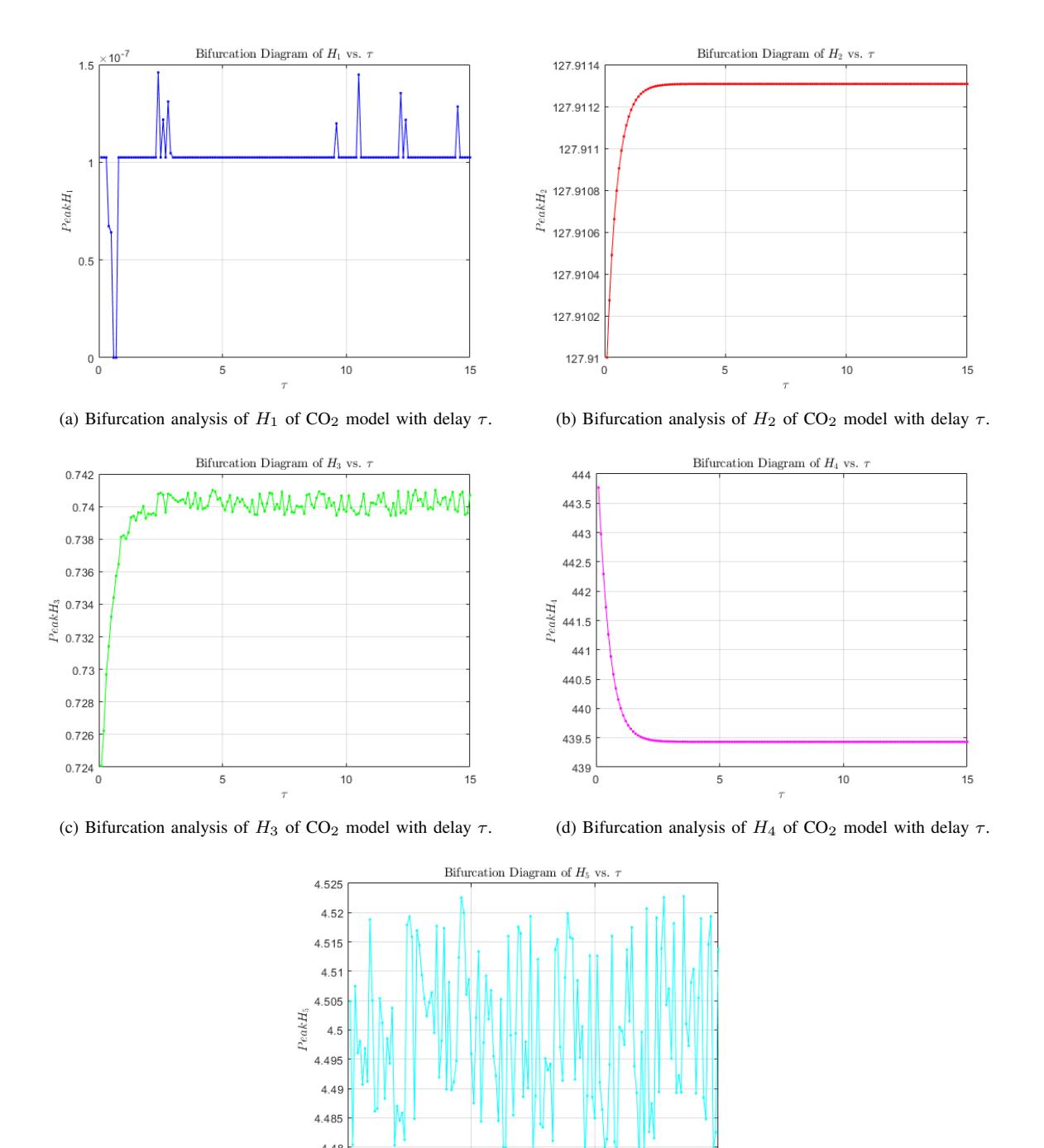
Figure 11: Bifurcation analysis of H1, H2, H3, H4, and H⁵ with delay τ .

(e) Bifurcation analysis of H⁵ of CO² model with delay τ

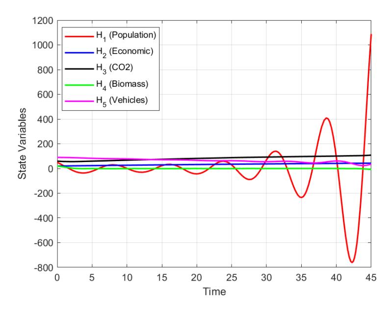
Figure 12: Dynamics of CO² model with delay τ .

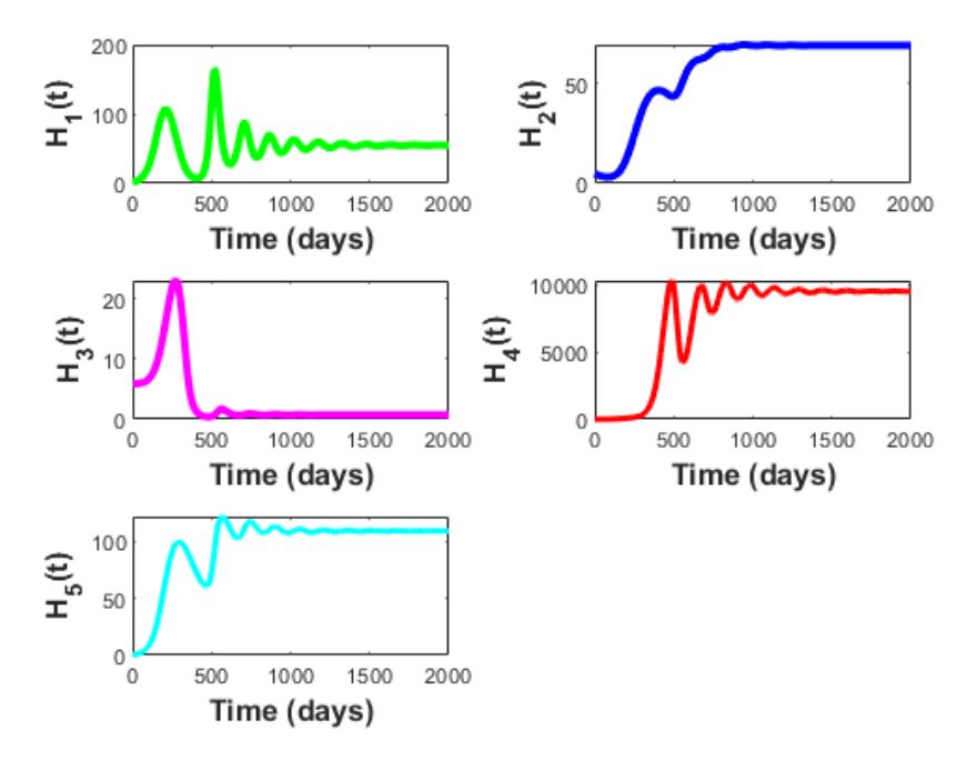
Figure 13: (a) Dynamics of CO² model with delay τ = 10.5.

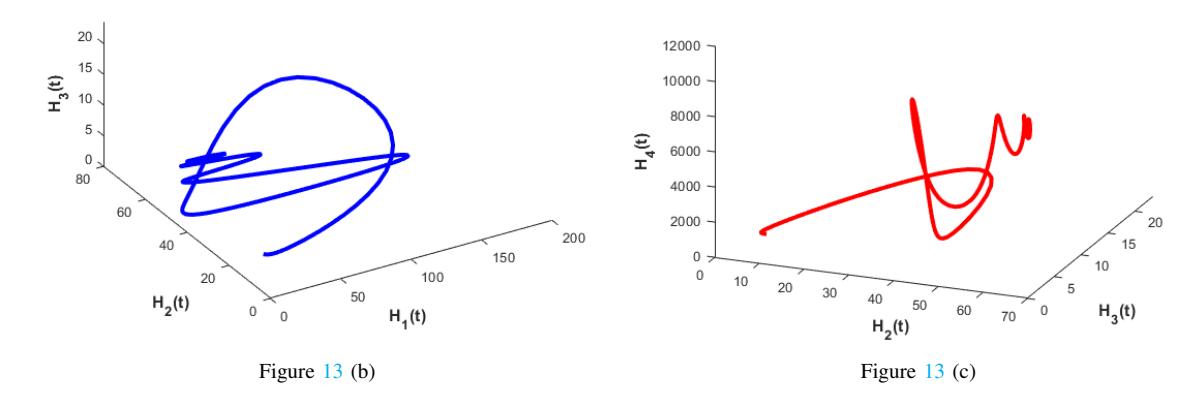
Figure 13 (b) represents the phase portrait of human population (H1), economic activities (H2) and Concentration of CO² in atmosphere (H3) and Figure 13 (c) represents the phase portrait of Concentration of CO² in atmosphere (H3) and human economic activities (H2)and biomass density of forest (H4) with the attributes of r¹ = 0.02; K = 1000; r² = 0.01; r³ = 0.02; r⁴ = 0.005; s¹ = 0.03; s² = 0.02; s³ = 0.01;t⁰ = 0.1;t¹ = 0.05;t² = 0.03;t³ = 0.02;t⁴ = 0.01; u¹ = 0.04;L = 500; u² = 0.005; v¹ = 0.02; v² = 0.01.

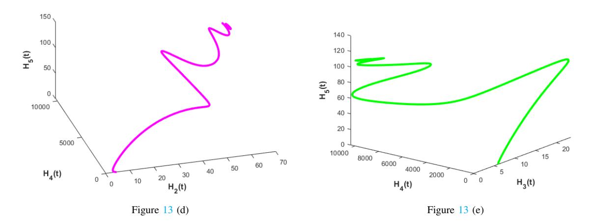
Figure 13 (d) represents the phase portrait of vehicle population (H5), biomass density of forest (H4) and economic activities (H2) and Figure 13 (e) represents the phase portrait of vehicle population (H5), biomass density of forest (H4) and concentration of CO² in atmosphere (H3) with the attributes of r¹ = 0.02; K = 1000; r² = 0.01; r³ = 0.02; r⁴ = 0.005; s¹ = 0.03; s² = 0.02; s³ = 0.01;t⁰ = 0.1;t¹ = 0.05;t² = 0.03;t³ = 0.02;t⁴ = 0.01; u¹ = 0.04;L = 500; u² = 0.005; v¹ = 0.02; v² = 0.01.

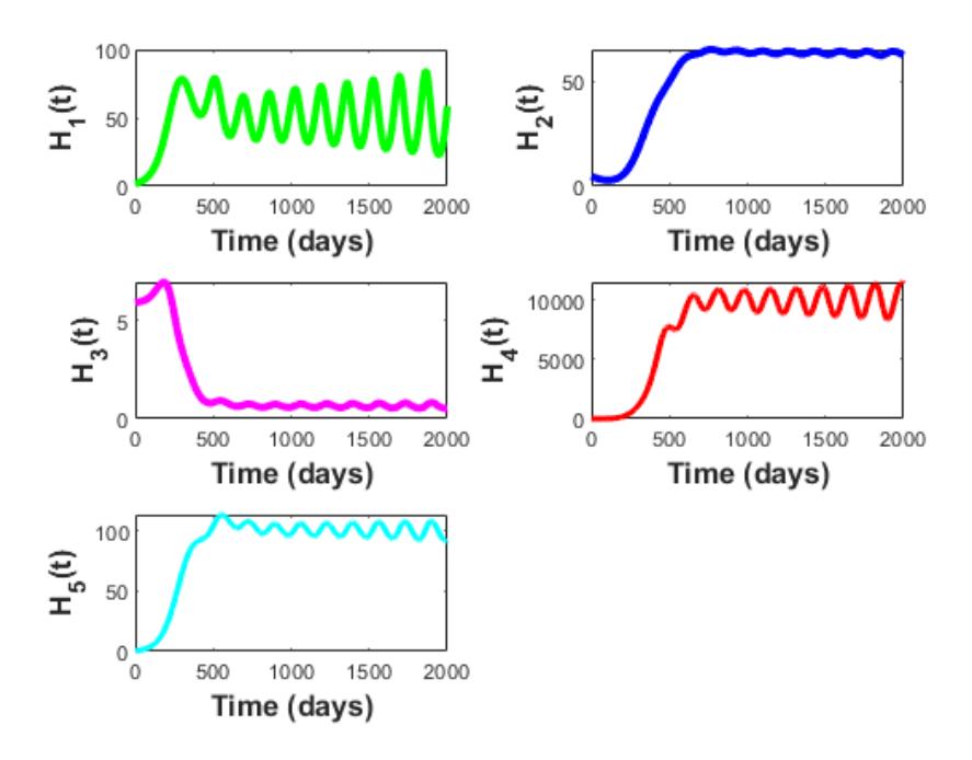
Figure 14: (a) Dynamics of CO² model with delay τ = 20.5.

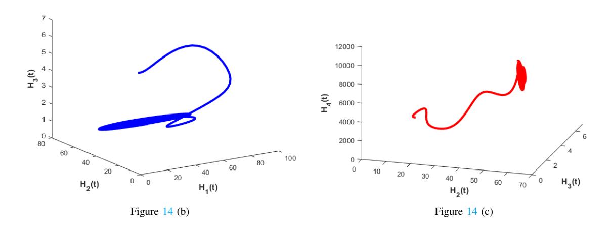
Figure 14 (b) represents the phase portrait of vehicle population (H3), biomass density of forest (H2) and human population (H1) and Figure 14 (c) represents the phase portrait of biomass density of forest (H4) human economic activities (H2)and concentration of CO² in atmosphere (H3) with the attributes of r¹ = 0.02; K = 1000; r² = 0.01; r³ = 0.02; r⁴ = 0.005; s¹ = 0.03; s² = 0.02; s³ = 0.01;t⁰ = 0.1;t¹ = 0.05;t² = 0.03;t³ = 0.02;t⁴ = 0.01; u¹ = 0.04;L = 500; u² = 0.005; v¹ = 0.02; v² = 0.01.

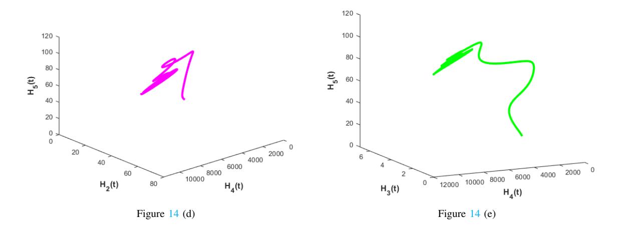
Figure 14 (d) represents the phase portrait of vehicle population (H5) economic activities (H2) and biomass density of forest (H4) and Figure 14 (e) represents the phase portrait of vehicle population (H5), concentration of CO² in atmosphere (H3) and biomass density of forest (H4) with the attributes of r¹ = 0.02; K = 1000; r² = 0.01; r³ = 0.02; r⁴ = 0.005; s¹ = 0.03; s² = 0.02; s³ = 0.01;t⁰ = 0.1;t¹ = 0.05;t² = 0.03;t³ = 0.02;t⁴ = 0.01; u¹ = 0.04;L = 500; u² = 0.005; v¹ = 0.02; v² = 0.01.

exhibits the most dynamic behavior with respect to the delay τ . For small τ , the peak value is around 4.5. As τ increases, the peak value shows significant fluctuations and potentially oscillatory behavior across the entire range of τ observed. The peak values vary between approximately 4.48 and 4.52, indicating that the long-term magnitude of the vehicle population is sensitive to the delay in the system, suggesting that the delay might induce or modulate oscillations in this variable.

Based on the bifurcation diagrams (Figure 11 (a)-(e)), it is observed that (i) H¹ (Human Population): Peak value remains very low (around 1 × 10⁻⁷ ) and relatively stable with respect to τ , with minor fluctuations. (ii) H² (Economic Activities): Peak value quickly stabilizes around 127.91 and remains largely unaffected by τ for τ > 1. (iii) H³ (CO² Concentration): Peak value quickly stabilizes around 0.74 and remains largely unaffected by τ for τ > 1. (iv) H⁴ (Forest Biomass): Peak value quickly stabilizes around 440 and remains largely unaffected by τ for τ > 1. (v) H⁵ (Vehicle Population): Shows significant fluctuations in its peak value as τ varies, indicating sensitivity to the delay and potential for delay-induced oscillations in this component of the system. The range of peak values is approximately 4.48 to 4.52.

Figure 12 illustrates the dynamic behavior of a CO² model, specifically showing the evolution of five state variables over time when a delay τ is introduced. The x-axis represents 'Time' (likely in arbitrary units), ranging from 0 to 45. The y-axis represents 'State Variables', with values ranging from approximately -800 to 1200. (i) H¹ (Population - Red Line): This variable exhibits significant oscillatory behavior throughout the observed time period. Initially, it hovers around zero, then shows damped oscillations, becoming more pronounced after approximately t = 20. After t ≈ 30, the oscillations appear to grow in amplitude, reaching a peak near t ≈ 40 and then undergoing a sharp decline to a large negative value around t ≈ 42, before dramatically increasing to over 1000 by t = 45. This suggests a highly unstable or chaotic population dynamic influenced by the delay. (ii) H² (Economic - Blue Line): Similar to H1, the economic variable also displays oscillations, but with generally smaller amplitudes compared to H1. It oscillates around zero for most of the simulation. Towards the end of the simulation, it remains relatively contained, not exhibiting the extreme fluctuations seen in H1. (iii) H³ (CO² - Black Line): The CO² variable shows a more stable and relatively steady behavior compared to H¹ and H2. It oscillates around a positive value (around 50 to 100) for the majority of the simulation. There's a slight increase in amplitude of oscillations around t = 30, but it eventually settles back. This suggests the CO² level might be relatively resilient to the same drastic fluctuations affecting population. (iv) H⁴ (Biomass - Green Line): The biomass variable

demonstrates very small oscillations close to zero throughout the entire time period. It appears to be relatively stable and unaffected by the significant swings in H1. (v) H⁵ (Vehicles - Magenta Line): The number of vehicles also shows stable behavior, oscillating around a constant positive value (around 50 to 100) with small amplitudes. Similar to biomass, it does not exhibit the dramatic changes seen in the population variable. In summary, Figure 12 indicates that the introduction of a delay τ into the CO² model leads to significant and potentially destabilizing oscillations, particularly for the population variable (H1), while other variables like CO2, biomass, and vehicles remain relatively more stable.

From Figures 13 (a) and 14 (a), it is found that the dynamics of the CO² model with a delay of τ = 10.5 and τ = 20.5 days respectively reveals complex interactions and temporal behaviors among its components as follows: (i) Oscillatory Behavior (H1(t) and H4(t)): The sustained oscillations suggest a dynamic equilibrium influenced by time-delayed feedback mechanisms. This could represent cyclical relationships within the carbon cycle, such as predator-prey dynamics or resource limitations. The delay of 20.5 days likely contributes significantly to these periodic behaviors.(ii) Stable Plateau (H2(t) and H5(t)): The initial growth followed by a plateau indicates that these components likely reach saturation or are limited by other factors within the system. The minor oscillations around the plateau could be a response to the fluctuations in other interacting variables. These might represent the capacity of certain carbon reservoirs.(iii) Transient Behavior (H3(t)): The rapid decline of H3(t) suggests it might be a quickly consumed reactant or an intermediate product in the CO² dynamics. Its near-zero steady state implies a significant role in the initial phase but less impact on the long-term behavior. The small final oscillations might be due to weak coupling with other oscillating components.

The fact that the phase portraits from Figures 13 (b), (c), (d), (e), Figures 14 (b), (c), (d), (e) are generated numerically implies that the underlying model consists of a system of differential equations that were solved using computational methods with the given parameter values. The specific shapes and behaviors observed in the phase portraits are direct outcomes of these equations and parameter settings. The numerical simulations, visualized through these phase portraits, reveal a complex and interconnected dynamical system involving human economic activities, vehicle population, and forest biomass. The bounded but intricate trajectories suggest ongoing, potentially non-periodic interactions between these variables, highlighting the non-trivial dynamics arising from the underlying model equations and the chosen parameter values. A deeper understanding of the model's equations and the role of the unspecified variable H2(t) would be necessary for a more comprehensive interpretation.

5. SUMMARY AND CONCLUSIONS

In this study a dynamic mathematical model has been formulated to explore the complex interplay between human activities and CO² emissions within the agricultural context. The model employs a system of differential equations to describe the interactions among key components: human population growth H1, human economic activities H2, atmospheric CO² concentration H3, forest biomass density H4, and vehicle population (H5). The model captures critical processes such as deforestation, economic outputs, and vehicular emissions contributing to CO² levels, along with the counterbalancing role of forest biomass in carbon sequestration. Parameters in the model account for natural growth rates, carrying capacities, and interaction coefficients that reflect both the aggravation and mitigation of CO² emissions. Moreover, the incorporation of a delay parameter τ allows for the modeling of temporal lags in the impacts of population dynamics and deforestation activities. This framework provides valuable insights into the dynamic feedback mechanisms and interactions that shape CO² emissions over time. The model emphasizes the importance of adopting sustainable practices and implementing effective policies to reduce environmental degradation, particularly within agricultural systems.

ACKNOWLEDGEMENT

The Department of Interdisciplinary Sciences, NIFTEM Knowledge Centre, NIFTEM and Department of Mathematics, School of Advanced Sciences, Vellore Institute of Technology have all provided invaluable assistance. The NIFTEM-K Communication Number is NIFTEM-P-2025-143.