

1. INTRODUCTION
Coronavirus disease 2019 (COVID-19), caused by the novel severe acute respiratory syndrome coronavirus 2 (SARS-CoV-2), emerged as a global pandemic in early 2020. Its rapid transmission, high morbidity and mortality rates, and profound socioeconomic impacts necessitated urgent and coordinated responses from governments, healthcare systems, and researchers worldwide [25].
Thailand was among the first countries outside China to report a COVID-19 case, with its first confirmed infection detected on January 13, 2020, at Suvarnabhumi Airport. The first COVID-19–related death was recorded on March 1, 2020. In response to the initial outbreak, the Thai government implemented rapid and stringent containment measures. During the first wave, which peaked in late March 2020 with approximately 188 daily cases linked to nightlife venues and boxing stadiums, nationwide lockdowns, curfews, travel restrictions, and mask mandates were enforced, effectively suppressing transmission [2].
Following the containment of the initial wave, Thailand experienced a resurgence in December 2020 originating from a seafood market in Samut Sakhon, where clusters among migrant workers reignited community transmission. This outbreak peaked in January 2021, with daily cases exceeding 900 before stabilizing in February. Subsequently, a more severe wave emerged in April 2021, driven by the Alpha variant and associated with entertainment venues in Bangkok. Daily infections surpassed 1,000, overwhelming healthcare facilities and necessitating the deployment of field hospitals to accommodate patient overflow [2]
Vaccination efforts commenced in early 2021. Initially, the government secured 26 million doses of the AstraZeneca vaccine and 2 million doses of Sinovac, later expanding procurement to include additional vaccine platforms. Domestic vaccine candidates, including ChulaCov19 and NDV-HXP-S, entered clinical trials by mid-2021. However, the emergence of the highly transmissible Delta variant triggered a major outbreak, pushing cumulative case counts beyond one million and placing unprecedented strain on the healthcare
∗Corresponding Author
Received July 10th, 2025, Revised September 6th, 2025, Accepted for publication November 18th, 2025. Copyright ©2025 Published by Indonesian Biomathematical Society, e-ISSN: 2549-2896, DOI:10.5614/cbms.2025.8.2.6
system. This situation prompted large-scale booster vaccination campaigns, particularly among individuals who had received inactivated vaccines [2].
During 2022 and 2023, the Omicron variant became the predominant strain in Thailand. Although significantly more contagious, it was generally associated with milder clinical outcomes. Consequently, Thailand transitioned from aggressive suppression strategies toward adaptive disease management. Public health restrictions were gradually relaxed, and COVID-19 began to be managed as an endemic disease. Sustained vaccination efforts and continued public adherence to basic preventive measures enabled the healthcare system to accommodate periodic surges without severe disruption [2].
By early 2025, COVID-19 was officially classified as an endemic disease in Thailand. Nevertheless, notable surges continued to occur, particularly during the rainy season and school terms. In May 2025, a significant outbreak was reported, with over 31,000 new weekly cases recorded between May 11-17, followed by more than 67,000 cases and eight deaths the subsequent week. At that time, the Omicron subvariant JN.1 accounted for approximately 64% of sequenced cases, while a newly emerging subvariant, NB.1.8.1, contributed to a sharp increase in infections. By May 30, cumulative cases for the year had reached 257,280, with 52 deaths. As of June 11, total reported cases had risen to 439,527, with 130 fatalities and weekly infections exceeding 100,000, particularly in Bangkok and Chonburi. Despite the surge, public health authorities indicated that the epidemic peak had passed [25].
Among the critical tools employed in the fight against COVID-19, mathematical modeling has played a pivotal role in understanding and controlling the disease's spread. Mathematical models offer a structured approach to simulating the transmission dynamics of infectious diseases. They enable researchers to estimate key epidemiological parameters, analyze disease progression, and assess the potential impacts of public health interventions such as lockdowns, quarantines, social distancing, and vaccination programs. Since the start of the pandemic, a variety of modeling frameworks—ranging from classical compartmental models like SIR (Susceptible–Infectious–Recovered) to sophisticated, data-driven, and stochastic models—have been developed and applied globally to inform policy and guide resource allocation.
As the pandemic has progressed into its endemic phase, modeling approaches have continued to evolve, incorporating more complex dynamics and exploring the interplay of multiple factors influencing disease transmission and control. For instance, Al-Arydah [3] extended the SVIR model by incorporating behavioral dynamics, distinguishing between individuals who act cautiously and those who become complacent. Their study emphasized the critical role of behavioral responses and included optimal control strategies to curb transmission. Further expanding the scope, recent models have investigated co-infection dynamics. A 2024 study analyzed the simultaneous spread of COVID-19 and leptospirosis, revealing increased morbidity among co-infected individuals and highlighting the need for integrated disease management strategies. Similarly, Appiah et al. [4] developed a co-infection model for tuberculosis and COVID-19, which incorporated optimal vaccination strategies alongside a cost-effectiveness analysis.
In the context of Thailand, Jose et al. [12] proposed a fractional-order SEIR model using Caputo derivatives, capturing memory effects and illustrating the influence of non-pharmaceutical interventions on outbreak trajectories. Their work offered nuanced insights into the epidemic's evolution within the Thai population. Comparative modeling studies have also emerged to support model selection and improve predictive accuracy. Mart´ınez-Fernandez et al. [ ´ 19] evaluated multiple compartmental models, examining their structural assumptions and predictive capabilities. Likewise, Manabe et al. [18] introduced a data-driven, autoregressive model to forecast cyclical COVID-19 waves in Japan, demonstrating the practical application of time-series models in real-time policy planning.
A broader synthesis of modeling efforts was presented by Demongeot and Magal [16], who reviewed over 230 studies encompassing compartmental, age-structured, phenomenological, and forecasting frameworks. Their comprehensive survey reflects the diversity and progression of modeling strategies employed throughout the pandemic. These advancements underline the vital role of mathematical modeling in responding to evolving epidemiological conditions. As the world adapts to living with COVID-19, new modeling approaches are needed to address ongoing challenges—particularly strategies that balance normalcy with effective disease mitigation. This study contributes to that effort by focusing on medical treatment strategies aimed at reducing the infectiousness of symptomatic and severe cases in Thailand's current epidemic context.
Mathematical models have played a critical role throughout the COVID-19 pandemic, offering valuable tools for forecasting disease trajectories, evaluating intervention strategies, and informing public health policies. Numerous studies [21], [10], [14], [27], [15], [17], [24], [6], [9] have demonstrated the utility of such models in assessing the impact of delayed interventions, healthcare system limitations, and behavioral responses. However, the reliability of these models depends heavily on the accuracy of their assumptions, the quality and timeliness of available data, and the capacity to incorporate real-world complexities, including asymptomatic transmission, time-dependent transmission rates, and the potential for reinfection.
Previous models have primarily focused on preventive measures such as vaccination, social distancing, lockdowns, and other protective strategies aimed at reducing the risk of infection among susceptible individuals. Some related studies have also incorporated control strategies targeting infected individuals. For instance, Alemzewde Ayalew et al. [5] proposed a model that included treatment controls for quarantined individuals. In their framework, the quarantine class represented infected people who had isolated themselves, and treatment for this group was effectively the same as for general infected cases. However, the model did not account for severe COVID-19 cases.
More recently, Bernard Asamoah Afful et al. [1] developed a deterministic optimal control compartmental model for COVID-19 that integrated a wide range of interventions. These included preventive controls such as social/physical distancing, mask wearing, handwashing, and hygiene education for susceptible individuals, along with vaccination strategies for susceptibles and treatment improvement controls for quarantined, asymptomatic, and infected cases. Despite its breadth, the study excluded severe cases from its framework. In addition, the definition of "preventive measures" lacked clarity, as it encompassed multiple interventions without distinguishing their individual characteristics. Similarly, the model applied a uniform treatment control across all infected classes, even though treatment approaches in reality would differ depending on disease severity. Another related study by Congyang Liu et al. [13] examined COVID-19 dynamics using a delayed SEIR model. They investigated control strategies involving social distancing and treatment of infected individuals, while vaccination was not considered. Their findings highlighted that pharmacological interventions were most effective for hospitalized patients. However, the model did not differentiate between severity levels of infection.
Collectively, these studies demonstrate substantial progress in integrating preventive and treatment-oriented control measures. However, none explicitly address treatment strategies stratified by disease severity, particularly for patients with Severe Acute Respiratory Infection (SARI). SARI is characterized by acute onset of fever exceeding 38 °C, cough within the preceding 10 days, and the need for hospitalization. Importantly, SARI may result from diverse etiologies, including viral pathogens such as influenza, respiratory syncytial virus (RSV), adenovirus, MERS, and SARS-CoV-2, as well as non-viral infections [25].
In 2025, Thailand's public health policy transitioned to a symptom-based approach emphasizing individual responsibility. Mandatory quarantines were replaced with guidance advising symptomatic individuals to selfisolate until they were fever-free for at least 24 hours without antipyretic medication, followed by five days of mask use. Individuals with known exposure were encouraged to undergo testing within 3-5 days. Preventive practices-including hand hygiene, mask use in crowded settings, and routine self-testing-were actively promoted, while booster vaccinations were strongly recommended for high-risk populations [2].
In response to evolving public health strategies, this study employs mathematical modeling to assess the effectiveness of Thailand's current approach to managing the ongoing COVID-19 epidemic. Our analysis highlights the impact of treating symptomatic cases and patients with Severe Acute Respiratory Infection (SARI) on reducing infectiousness and transmission, in contrast to approaches that rely predominantly on conventional measures such as vaccination and social distancing.
This paper presents a mathematical model that integrates medical treatment as a central control strategy and examines its impact on disease transmission. We analyze the stability of disease-free and endemic equilibrium points and explore an optimal control framework for evaluating treatment-based interventions. The goal is to provide insights into the dynamics of COVID-19 under current endemic conditions and to support data-driven public health decision-making for sustained management of the disease.
2. MODEL FORMULATION
For the formulation of our model, let N denote the total human population. The population is divided into four distinct compartments: susceptible individuals (S), asymptomatic infectious individuals (I1), symptomatic infectious individuals (I2), and individuals with Severe Acute Respiratory Infection (SARI) (A). We introduce two control parameters, ϕ1 and ϕ2, representing the treatment rates for symptomatic and Severe Acute Respiratory Infection, respectively.
Based on these classifications and control measures, the proposed model is defined as shown in Figure 1.
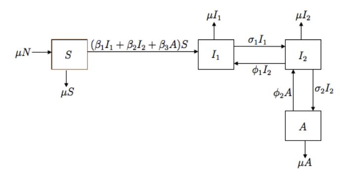
Figure 1: The schematic representation of the proposed model.
\[\frac{dS}{dt} = \mu N - (\beta_1 I_1 + \beta_2 I_2 + \beta_3 A) S - \mu S, \tag{1}\]
\[\frac{dI_1}{dt} = (\beta_1 I_1 + \beta_2 I_2 + \beta_3 A)S - \mu I_1 - \sigma_1 I_1 + \phi_1 I_2, \tag{2}\]
\[\frac{dS}{dt} = \mu N - (\beta_1 I_1 + \beta_2 I_2 + \beta_3 A) S - \mu S, \tag{1}\] \[\frac{dI_1}{dt} = (\beta_1 I_1 + \beta_2 I_2 + \beta_3 A) S - \mu I_1 - \sigma_1 I_1 + \phi_1 I_2, \tag{2}\] \[\frac{dI_2}{dt} = \sigma_1 I_1 - \mu I_2 - \sigma_2 I_2 - \phi_1 I_2 + \phi_2 A, \tag{3}\] \[\frac{dA}{dt} = \sigma_2 I_2 - \mu A - \phi_2 A. \tag{4}\]
\[\frac{dA}{dt} = \sigma_2 I_2 - \mu A - \phi_2 A. \tag{4}\]
The vector form of the above equations is given by:
\[\frac{dX}{dt} = F(X), \text{ with } X = (S, I_1, I_2, A)^T.\] (5)
The parameters and symbols used in the model are summarized in Table 1.
Table 1: Parameters and symbols.
| Parameter | Symbols |
|---|---|
| Susceptible population | S |
| Asymptomatic COVID-19 infectious state | \(I_1\) |
| Symptomatic COVID-19 infectious state | \(I_2\) |
| Severe acute respiratory infectious state | A |
| Total population | N |
| Natural birth and natural death rate | \(\mu\) |
| Transmission coefficient of the infectious initially | \(\dot{\beta}_1\) |
| Transmission coefficient of the infectious the second stage | \(\beta_2\) |
| Transmission coefficient of the severe cases | \(\beta_3\) |
| Progression rate from \(I_1\) to \(I_2\) infection | \(\sigma_1\) |
| The state of \(I_2\) becomes \(A\) | \(\sigma_2\) |
| Medication rate for asymptomatic patients | \(\phi_1^-\) |
| Medication rate for Severe Acute Respirator Infection | \(\phi_2\) |
3. MODEL ANALYSIS
We begin our analysis by examining the disease-free equilibrium (DFE) and calculating the basic reproduction number. This is done by setting \(I_1 = I_2 = A = 0\) in the model equations and solving for S. Under these conditions, Equation (1) reduces to N=S since \(\mu \neq 0\). Thus, the DFE is denoted by:
\[\epsilon_0 = (N, 0, 0, 0).\]
Next, we compute the basic reproduction number, \(R_0\), for the model using the next-generation matrix method proposed by van den Driessche and Watmough, and the reproduction number for the model is
\[R_{0} = T^{*} = \frac{\beta_{1}N((\mu + \sigma_{2} + \phi_{1})(\mu + \phi_{2}) + \sigma_{2}\phi_{2})}{Q} + \frac{\beta_{2}N\sigma_{1}(\mu + \phi_{2})}{Q} + \frac{\beta_{3}N\sigma_{1}\sigma_{2}}{Q},\] \[= \frac{\beta_{1}N((\mu + \sigma_{2} + \phi_{1})(\mu + \phi_{2}) + \sigma_{2}\phi_{2}) + \beta_{2}N\sigma_{1}(\mu + \phi_{2}) + \beta_{3}N\sigma_{1}\sigma_{2}}{(\mu + \sigma_{1})(\mu + \sigma_{2} + \phi_{1})(\mu + \phi_{2}) - \sigma_{2}\phi_{2}(\mu + \sigma_{1}) - \sigma_{1}\phi_{1}(\mu + \phi_{2})},\] \[= \frac{\beta_{1}N((\mu + \sigma_{2} + \phi_{1})(\mu + \phi_{2}) + \sigma_{2}\phi_{2})}{D} + \frac{\beta_{2}N\sigma_{1}(\mu + \phi_{2})}{D} + \frac{\beta_{2}N\sigma_{1}\sigma_{2}}{D},\] \[= R_{I_{1}} + R_{I_{2}} + R_{A},\] where \(D = (\mu + \sigma_1)(\mu + \sigma_2 + \phi_1)(\mu + \phi_2) - \sigma_2\phi_2(\mu + \sigma_1) - \sigma_1\phi_1(\mu + \phi_2)\), see Appendix A for details. The basic reproduction number can be decomposed into three additive components, \(R_0 = R_{I_1} + R_{I_2} + R_A\). Here, \(R_{I_1}\) reflects transmission from asymptomatic infections, \(R_{I_2}\) captures transmission from symptomatic cases, and \(R_A\) represents transmission from SARI cases. Each term is scaled by the probability of progression through disease stages, treatment rates, and natural exit, while the denominator accounts for the average duration of infectiousness across compartments. This decomposition highlights the relative importance of mild, moderate, and severe infections in sustaining transmission, and illustrates how treatment and progression parameters shape epidemic potential.
Based on the work in [11], we immediately obtain the result below:
Theorem 3.1. The disease-fee equilibrium of the model is locally asymptotically stable if \(R_0 < 1\), and unstable if \(R_0 > 1\).
To investigate the global asymptotic stability of the disease-free equilibrium (DFE), a common approach is to construct a suitable Lyapunov function. However, in this study, we adopt a simpler method based on a result introduced by Castillo-Chavez et al [7].
Lemma 3.2. Consider a model system written in the form
\[\frac{dX_1}{dt} = F(X_1, X_2), \tag{6}\]
\[\frac{dX_1}{dt} = F(X_1, X_2), (6)\] \[\frac{dX_2}{dt} = G(X_1, X_2), G(X_1, 0) = 0, (7)\] where \(X_1 \in \mathbb{R}^m\) denotes (its components) the number of uninfected individuals and \(X_2 \in \mathbb{R}^n\) denotes (its components) the number of infected individuals including latent, infectious, etc; \(X_0 = (X_1^*)\) denotes the disease-free equilibrium of the system.
Also assume the conditions (H1) and (H2) below:
(H1) For \(\frac{dX_1}{dt} = F(X_1^*, 0)\) is globally asymptotically stable; (H2) \(G(X_1, X_2) = AX_2 - \hat{G}(X_1, X_2)\), \(\hat{G}(X_1, X_2) \geq 0\) for \((X_1, X_2) \in \Omega\), where the Jacobian \(A = \frac{\partial G}{\partial X_2}(X_1^*, 0)\) is an M-matrix (the off diagonal elements of A are nonnegative) and \(\Omega\) is the region where the model makes biological sense. Then the DFE \(X_0 = (X_1^*, 0)\) is globally asymptotically stable provided that \(R_0 < 1\).
Theorem 3.3. The disease-free equilibrium of the model is globally asymptotic stable if \(R_0 < 1\).
Proof: See Appendix B.
The stability of the disease-free equilibrium (DFE) governs the short-term epidemic behavior of the disease, while the long-term dynamics are characterized by the stability of the endemic equilibrium. In this section, we analyze the endemic properties of our model.
When the disease is presence in the population, \(I_1^*\) and \(I_2^* \neq 0\), there may be several critical points, which are the endemic equilibrium points (EEP) of the model. These points will be denoted as \(\varepsilon_0^* = (S^*, I_1^*, I_2^*, A^*)\)
and are determined from the model as follows
\[\frac{dS^*}{dt} = \mu N - \beta_1 I_1^* S^* - \beta_2 I_2^* S^* - \beta_3 A^* S^* - \mu S^*, \tag{8}\]
\[\frac{dI_{1*}}{dt} = \beta_{1}I_{1}^{*}S^{*} + \beta_{2}I_{2}^{*}S^{*} + \beta_{3}A^{*}S^{*} - \mu I_{1}^{*} - \sigma_{1}I_{1}^{*} + \phi_{1}I_{2}^{*}, \qquad (9)\] \[\frac{dI_{2*}}{dt} = \sigma_{1}I_{1}^{*} - \mu I_{2}^{*} - \sigma_{2}I_{2}^{*} - \phi_{1}I_{2}^{*} + \phi_{2}A^{*}, \qquad (10)\] \[\frac{dA*}{dt} = \sigma_{2}I_{2}^{*} - \mu A^{*} - \phi_{2}A^{*}. \qquad (11)\]
\[\frac{dI_{2*}}{dt} = \sigma_{1}I_{1}^{*} - \mu I_{2}^{*} - \sigma_{2}I_{2}^{*} - \phi_{1}I_{2}^{*} + \phi_{2}A^{*}, \tag{10}\]
\[\frac{dA^*}{dt} = \sigma_2 I_2^* - \mu A^* - \phi_2 A^* . \tag{11}\]
First, we find \(S^*\) from Equation (8), we have
\[\mu N - \beta_1 I_1^* S^* - \beta_2 I_2^* S^* - \beta_3 A^* S^* - \mu S^* = 0,\] \[\beta_1 I_1^* S^* + \beta_2 I_2^* S^* + \beta_3 A^* S^* + \mu S^* = \mu N,\] \[S^* (\beta_1 I_1^* + \beta_2 I_2^* + \beta_3 A^* + \mu) = \mu N,\] \[S^* = \frac{\mu N}{\beta_1 I_1^* + \beta_2 I_2^* + \beta_3 A^* + \mu}.\] (12)
Substitute of \(A^*\) in Equation (12), we have
\[S^* = \frac{\mu N}{\beta_1 I_1^* + \beta_2 I_2^* + \beta_3 \left(\frac{\sigma_2 I_2^*}{\mu + \beta_2}\right) + \mu},\tag{13}\]
Next, to find \(I_1^*\) from Equation (9), we have
\[\beta_{1}I_{1}^{*}S^{*} + \beta_{2}I_{2}^{*}S^{*} + \beta_{3}A^{*}S^{*} - \mu I_{1}^{*} - \sigma_{1}I_{1}^{*} + \phi_{1}I_{2}^{*} = 0,\] \[\mu I_{1}^{*} + \sigma_{1}I_{1}^{*} - \beta_{1}I_{1}^{*}S^{*} = \beta_{2}I_{2}^{*}S^{*} + \phi_{1}I_{2}^{*} + \beta_{3}A^{*}S^{*},\] \[I_{1}^{*}(\mu + \sigma_{1} - \beta_{1}S^{*}) = (\beta_{2}S^{*} + \phi_{1})I_{2}^{*} + \beta_{3}A^{*}S^{*},\] \[I_{1}^{*} = \frac{(\beta_{2}S^{*} + \phi_{1})I_{2}^{*} + \beta_{3}A^{*}S^{*}}{\mu + \sigma_{1} - \beta_{1}S^{*}}.\] (14)
Next, to find \(I_2^*\) from Equation (10), we have
\[\sigma_{1}I_{1}^{*} - \mu I_{2}^{*} - \sigma_{2}I_{2}^{*} - \phi_{1}I_{2}^{*} + \phi_{2}A^{*} = 0\] \[\mu I_{2}^{*} + \sigma_{2}I_{2}^{*} + \phi_{1}I_{2}^{*} = \sigma_{1}I_{1}^{*} + \phi_{2}A^{*}\] \[I_{2}^{*} = \frac{\sigma I_{1}^{*} + \phi_{2}A^{*}}{\mu + \sigma_{2} + \phi_{1}}.\] (15)
Substitute of \(A^*\) in Equation (15), we have
\[I_2^* = \frac{\sigma I_1^* + \phi_2(\frac{\sigma_2 I_2^*}{\mu + \phi_2})}{\mu + \sigma_2 + \phi_1},\]
and
\[I_1^* = \frac{I_2^*(\mu + \sigma_2 + \phi_1) - \phi_2(\frac{\sigma_2 I_2^*}{\mu + \phi_2})}{\sigma_1}.\] (16)
Next, to find \(A^*\) from Equation (11), we have
\[\sigma_{2}I_{2}^{*} - \mu A^{*} - \phi_{2}A^{*} = 0,\] \[\mu A^{*} + \phi_{2}A^{*} = \sigma_{2}I_{2}^{*},\] \[A^{*}(\mu + \phi_{2}) = \sigma_{2}I_{2}^{*},\] \[A^{*} = \frac{\sigma_{2}I_{2}^{*}}{\mu + \phi_{2}}.\] (17)
We first show the following theorem.
Theorem 3.4. The positive endemic equilibrium \(\epsilon^*\) of the system (8) - (11) exists and unique if \(R_0 > 1\), and there is no positive endemic equilibrium if \(R_0 < 1\).
3.1. Local Stability
We now proceed to analyze the stability properties of the endemic equilibrium. First, we establish the following result concerning its local stability.
Theorem 3.5. The positive endemic equilibrium \(\varepsilon^*\) is locally asymptotically stable.
4. SIMULATION WITH OPTIMAL CONTROL STUDY
In this section, we will use the following theorem to apply optimal control theory to seek cost effective treatment programs for our model.
4.1. Pontryagin's Maximum/Minimum Principle
These conclusions can be extended to a version of Pontryagin's Maximum/Minimum Principle [20].
Theorem 4.1. If \(u^*(t)\) and \(x^*(t)\) are optimal for Equations (1)-(4), then there exists a piece-wise differentiable adjoint variable \(\lambda(t)\) such that
\[H(t, x^*(t), u(t), \lambda(t)) \le H(t, x^*(t), u^*(t), \lambda(t)),\] for all control u at each time t, where the Hamiltonian H is
\[H = f(t, x(t), u(t)) + \lambda(t)g(t, x(t), u(t)),\] and
\[\lambda'(t) = -\frac{\partial H(t, x^*(t), u^*(t), \lambda(t))}{\partial x}, \lambda(t_1) = 0.\]
Theorem 4.2. Suppose that f(t,x,u) and g(t,x,u) are both continuously differentiable functions in their three arguments and concave in u. Suppose \(u^*\) is an optimal control for problem (1)-(4), with associated state \(x^*\), and \(\lambda\) a piece-wise differentiable function with \(\lambda \geq 0\) for all t. Suppose for all \(t_0 \leq t \leq t_1\)
\[0 = H_u(t, x^*(t), u^*(t), \lambda(t)).\]
Then for all controls u and each \(t_0 \le t \le t_1\), we have
\[H(t, x^*(t), u(t), \lambda(t)) \le H(t, x^*(t), u^*(t), \lambda(t)).\]
Now we turn to more general model with time-dependent controls \(\phi_1(t)\) and \(\phi_2(t)\). We consider the system on a time interval [0,T]. The function \(\phi_1(t)\) and \(\phi_2(t)\) are assumed to be at least Lebesgue measurable on [0,T]. The control set is defined as
\[\Omega = \{ \phi_1(t), \phi_2(t) | 0 \le \phi_1(t), \phi_2(t) \le \phi_{max} \},\\] where \(\phi_{max}\) denotes the upper bounds for the effort of medical treatments. The bound reflects practical limitation on the maximum rate of control in given time period.
4.2. Optimal Control Study
The inclusion of time-dependent control variables complicates the analytical study of the system, as the disease dynamics now evolve in response to the progression of these controls. To address this, we perform an optimal control analysis. Our objective is to minimize both the total number of infections and the associated control costs over the time interval [0, T], that is,
\[\min_{(\phi_{1,2})\in\Omega} \int_0^T \left[ I_1(t) + I_2(t) + A(t) + c_{11}\phi_1(t)I_2(t) + c_{12}\phi_1^2(t) + c_{21}\phi_2(t)A(t) + c_{22}\phi_2^2(t) \right] dt.\] (18)
Here, the parameters c11 , c12 , c21 and c22 with appropriate units, define the appropriate costs associated with these controls. The optimal control functions, derived from the objective function and the Hamiltonian (see Appendix E), are given as follows:
\[\phi_1(t) = \frac{\lambda_{I_2}(I_2) - c_{11}I_2(t) - \lambda_{I_1}I_2}{2c_{12}},\] and
\[\phi_2(t) = \frac{\lambda_A(A) - c_{21}A(t) - \lambda_{I_2}(A)}{2c_{22}}.\]
4.3. Numerical Results
Given the presence of initial conditions for the state equations, final-time conditions for the adjoint equations, and the nonlinear nature of the model, the optimal control system must be solved numerically. To this end, we employ the Forward-Backward Sweep Method to perform the numerical simulations.
Table 2: Description of parameters.
| Parameter | Symbol | Value | References |
|---|---|---|---|
| Total population | N | 10,000 | Assumed |
| Natural birth and natural death rate | µ | 1/(70 × 356) | [26] |
| Transmission rate of Asymptomatic patients | β1 | 0.05/N | Assumed |
| Transmission rate of Symptomatic patients | β2 | 0.3/N | Assumed |
| Transmission rate of SARI patients | β3 | 0.6/N | Assumed |
| Progression rate from I1 to I2 | σ1 | 0.25 | Assumed |
| The rate of becoming SARI patients from I2 to A | σ2 | 0.15 | Assumed |
In our simulation, we consider the spread of COVID-19 within a closed population, where individuals are initially unaware of the ongoing transmission. Given the current normalization of COVID-19 in daily life, many individuals lack adequate protective behaviors, making it easier for the disease to spread. We begin by assuming that asymptomatic individuals exhibit very mild or no symptoms and therefore are less likely to transmit the virus—for instance, they may not cough or sneeze, which reduces transmission in the absence of personal protection measures. This assumption is supported by several studies suggesting that while asymptomatic individuals can transmit COVID-19, their infectiousness is generally lower than that of symptomatic cases [22]. Assuming that, over time, most individuals may become infected, our objective is to maximize the proportion of asymptomatic cases while minimizing the treatment costs for symptomatic and SARI patients. To start, we consider a scenario in which treatment costs are relatively low, assigning values c11 = 1, c12 = 1, c21 = 1 and c22 = 1. The corresponding simulation results are presented in the following figures.
Figure 2 (a) illustrates the number of susceptible individuals over a 300-day simulation period. The figure shows a slow decline in the susceptible population when control measures are implemented. This indicates that medical treatment targeting symptomatic and SARI cases plays a significant role in slowing down the infection rate. Figure 2 (b) displays the number of asymptomatic individuals. Under the implementation of treatment controls for symptomatic and SARI cases, the number of asymptomatic infections remains relatively high. This aligns with our assumption that, in a closed population where individuals are unaware of the disease and do not take personal protective measures, symptomatic individuals are the most infectious. Therefore,
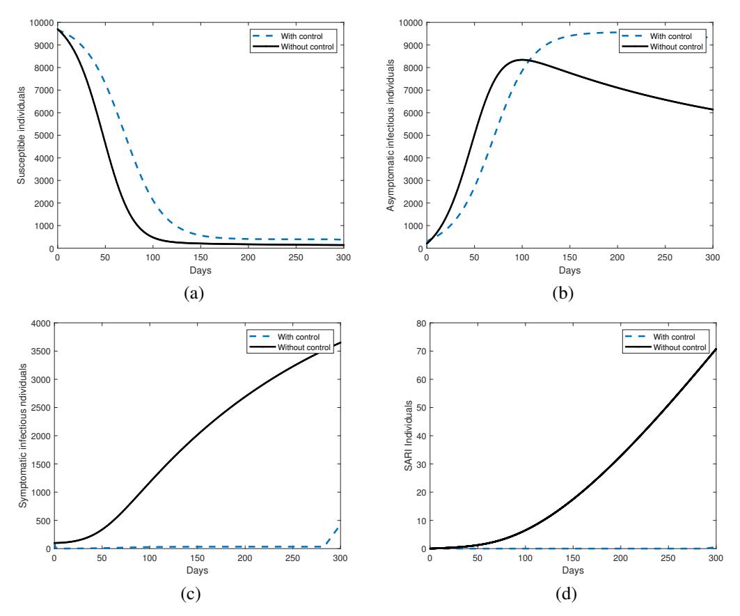
Figure 2: (a) Susceptible population, (b) Asymptomatic individuals, (c) Symptomatic patients, and (d) SARI patients.
reducing the number of symptomatic and SARI cases effectively slows disease transmission. Figures 2 (c) and 2 (d) show the number of symptomatic and SARI patients, respectively. These figures confirm that, with appropriate medication strategies—depicted in Figures 3 (a) and 3 (b)—the number of symptomatic and SARI cases remains low. Specifically, Figure 3 (a) suggests that approximately 70% of symptomatic patients should receive treatment consistently throughout the outbreak period. In contrast, Figure 3 (b) shows that around 70% of SARI cases should be treated intensively during the first 10 days, with treatment levels gradually declining to near zero after 100 days of infection.
In this scenario, we increase the treatment costs for symptomatic patients by setting \(c_{11}=10, c_{12}=10\), while keeping \(c_{21}=1\) and \(c_{22}=1\). Figures 4 (a) and 4 (b) illustrate the numbers of susceptible individuals and asymptomatic patients, respectively. Compared to the previous case, the results show subtle differences. Notably, after approximately 150 days, the number of asymptomatic individuals begins to decline, which can be attributed to the increased cost of treating symptomatic and SARI patients. As medical interventions become more limited due to higher costs, the number of symptomatic patients begins to rise around day 150, and the number of SARI cases increases significantly after approximately 270 days. This trend suggests that patients are at greater risk of progressing to more serious conditions, potentially resulting in higher mortality.
The control strategies for this scenario are illustrated in Figures 5 (a) and 5 (b). As shown in Figure 5 (a), medication coverage for symptomatic patients reaches up to 70% only until about 150 days after the outbreak onset, after which it declines due to the increased cost of implementation.
Next, we examine Case 3, where the medication costs for both symptomatic and SARI patients are increased to \(c_{11} = 10, c_{12} = 10, c_{21} = 10\) and \(c_{22} = 10\). As shown in Figures 6 (a) and 6 (b), the numbers of susceptible
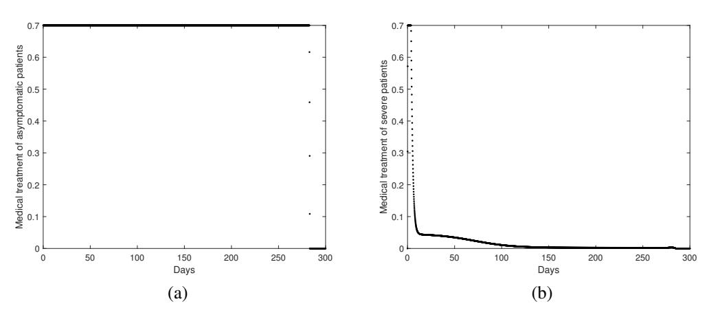
Figure 3: (a) Medication control for Symptomatic patients, and (b) Medication control for SARI patients.
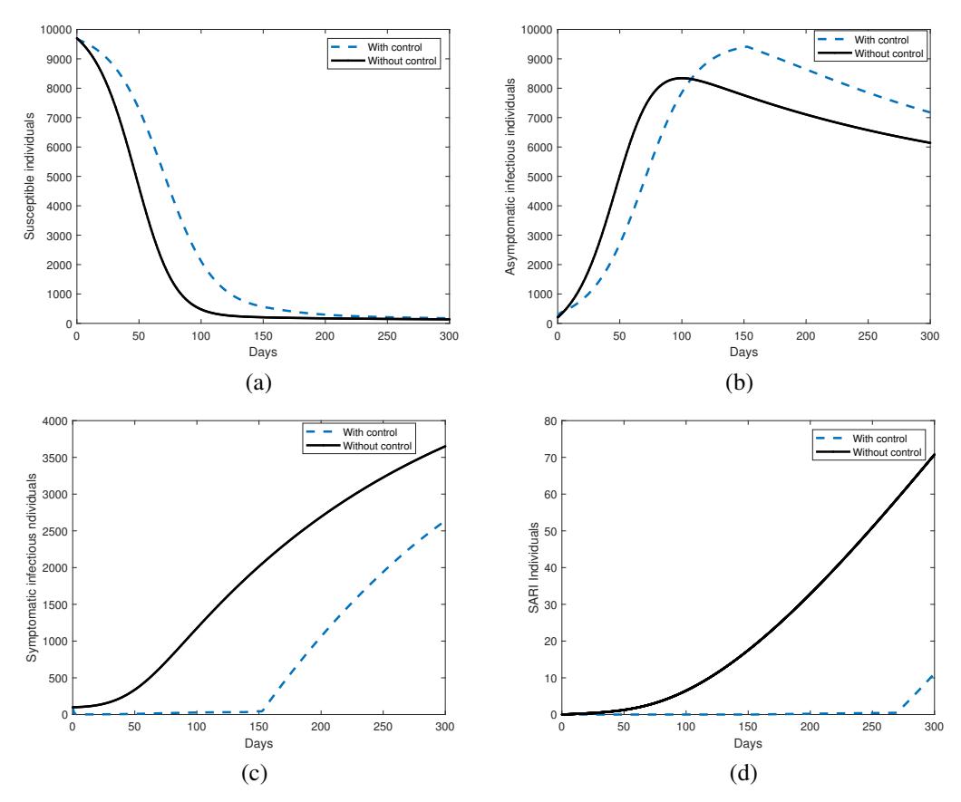
Figure 4: (a) Susceptible population, (b) Asymptomatic individuals, (c) Symptomatic patients, and (d) SARI patients.
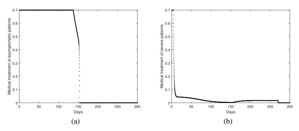
Figure 5: (a) Medication control for Symptomatic patients, and (b) Medication control for SARI patients.
and asymptomatic individuals remain similar to those observed in Case 2. This similarity is likely due to the relatively small number of SARI patients, so increasing treatment costs for this group does not significantly affect the overall outcome. Consequently, other state variables also exhibit comparable patterns, as illustrated in Figures 6 (c), 7 (a), and 7 (b).
We now turn our attention to investigating COVID-19 infections in Thailand. Using data collected from multiple sources [25], [8], [23], we compiled Thailand's COVID-19 case numbers from February to the first week of July 2025, as shown in Figure 8. The data suggest that Thailand has passed the peak of this season's outbreak. However, since the new school year began in June, the trend could change without effective control measures. In May, new infections peaked at approximately 170,000 cases, possibly influenced by the Songkran Festival in April, which likely contributed to increased transmission. In June, infections declined to about 130,000 new cases. Yet, within just the first few weeks of July, new infections rose again to nearly 100,000, indicating a potential resurgence by the end of the month.
To simulate COVID-19 dynamics in Thailand, we calibrated our model using this data. We set the total population N=60,000,000, with initial conditions \(S(0)=N-20,000,I_1(0)=20,000\), and \(I_2(0)=0,A(0)=0\), keeping other parameters unchanged. Since the available data pertains only to new infections, our model focuses on simulating new infection cases, corresponding to asymptomatic individuals.
Figure 9 compares the original model simulation (solid line) with the observed COVID-19 trend in Thailand from February to early July 2025, showing good agreement. The dashed line represents a control scenario where medication is applied to symptomatic and severe patients, significantly reducing case numbers relative to observed data. This suggests that, in reality, many people were not sufficiently aware or proactive in protecting themselves, delaying treatment, and maintaining close contact with others, thereby sustaining disease transmission.
Figure 10 offers valuable insight into how control measures impact the trajectory of the susceptible population during a COVID-19 outbreak. Under optimal control conditions, represented by the dashed line, the susceptible population declines steadily but at a slower rate. This slower decline indicates a more controlled spread of the infection, which is beneficial for several reasons.
First, a gradual decrease in the susceptible population helps prevent overwhelming the healthcare system. When infections rise too quickly, hospitals and medical staff can become overloaded, leading to reduced quality of care, increased mortality, and greater strain on resources. By flattening the curve, optimal control measures such as targeted medical treatment, isolation of symptomatic and SARI patients, and public health interventions help maintain the healthcare system's capacity to manage cases effectively. Second, the slower infection rate buys time for public health authorities to implement additional preventive strategies. This includes ramping up vaccination campaigns, enhancing testing and contact tracing, and increasing public awareness about protective behaviors like mask-wearing and social distancing. Such time is critical, especially in the context of emerging variants or seasonal fluctuations that can alter disease dynamics.
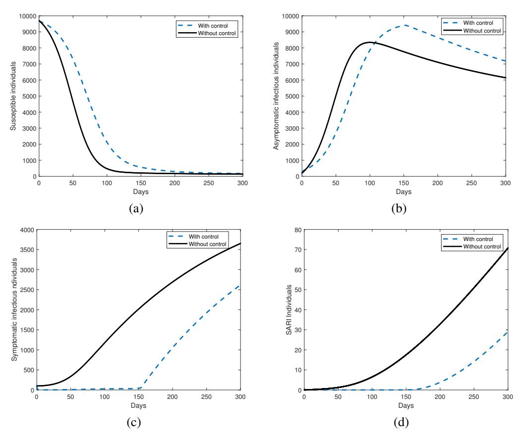
Figure 6: (a) Susceptible population, (b) Asymptomatic individuals, (c) Symptomatic patients, and (d) SARI patients.
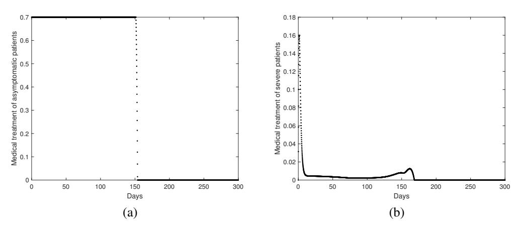
Figure 7: (a) Medication control for Symptomatic patients, and (b) Medication control for SARI patients.
COVID-19: Thailand 2025
180,000 160,000 140,000 120,000 108,000 100,000 80,000 60,000 40,000
April Figure 8: Thailand data for COVID-19 of January to the first week of July of 2025.
May
June
July
20,000
February
March
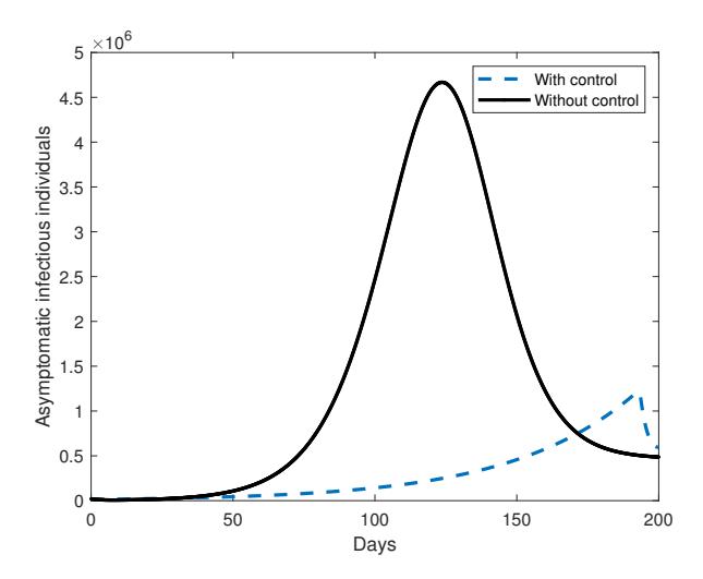
Figure 9: The simulation of Thailand's data for COVID-19 of 2025: Asymptomatic cases.
Conversely, the solid line in the figure shows the scenario without any control interventions. The rapid decline in susceptible individuals reflects widespread and uncontrolled transmission of the virus. This rapid spread accelerates community infection, quickly reducing the pool of people susceptible to infection but at the cost of high morbidity and mortality. Moreover, such an explosive outbreak can severely disrupt societal functions, including workforce availability, education, and economic stability. The contrast between these two scenarios underscores the crucial role of timely and effective disease control strategies. While some level of infection may be inevitable, managing the pace and scale of transmission is essential to reduce adverse health outcomes and societal disruption. Furthermore, this approach supports the transition of COVID-19 from a pandemic emergency toward a more manageable endemic state.
In conclusion, maintaining and optimizing control measures remains a key public health priority. Continuous monitoring of infection trends and adaptive implementation of interventions can help safeguard vulnerable populations, protect healthcare infrastructure, and minimize the broader impacts of COVID-19.
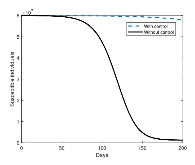
Figure 10: Thailand data for COVID-19 of January to the first week of July of 2025.
5. CONCLUSION
We have developed a mathematical model of COVID-19 incorporating optimal control strategies and analyzed the stability of both the disease-free and endemic equilibrium points. Additionally, we examined the optimal control problem focusing on medical treatment for symptomatic and SARI patients. Assuming a closed population where individuals are unaware of the disease and therefore do not engage in protective behaviors, the virus is free to spread unimpeded. Under these conditions, our model predicts a substantial number of infections in a large population, as exemplified by the case of Thailand.
However, the application of control measures such as medical treatment can significantly reduce the number of infections. In our simulations, we assume that asymptomatic individuals are less infectious than symptomatic and SARI cases; thus, a higher proportion of asymptomatic infections corresponds to a slower overall disease spread. It is important to note that our model does not include personal protective measures like mask-wearing or self-isolation, nor does it incorporate vaccination. Including these interventions would likely have a much greater impact on controlling transmission. Nevertheless, our primary objective is to explore the dynamics of living with the disease while implementing treatment strategies aimed at limiting outbreak severity.
Our model has certain limitations that can be refined in future work. One important consideration is the role of the SARI (Severe Acute Respiratory Infection) compartment. SARI refers to cases where patients develop acute respiratory illness with symptoms such as fever, cough, and difficulty breathing, which often require hospitalization and intensive care. In the context of COVID-19, SARI may arise not only from individuals who initially show mild to moderate symptoms but also from those who progress to severe disease.
A more realistic disease pathway would reflect that, after a susceptible individual contracts COVID-19, they may first become asymptomatic. Over time, some will develop symptoms, and a portion of these will worsen into severe illness. During this progression, if treatment is ineffective, both symptomatic and severe patients may transition into the SARI category. To address this limitation, our next study will expand the model to explicitly incorporate SARI dynamics, thereby improving its accuracy and applicability.
ACKNOWLEDGEMENT
This work was supported by Naresuan University (NU), and National Science, Research and Innovation Fund (NSRF), Grant NO. R2568B023.