Electronic Journal of Graph Theory and Applications

On energy, Laplacian energy and p-fold graphs

Hilal A. Ganie^a, S. Pirzada^b, Edy Tri Baskoro^c

hilahmad1119kt@gmail.com, pirzadasd@kashmiruniversity.ac.in, ebaskoro@math.itb.ac.id

For a graph G having adjacency spectrum (A-spectrum) \(\lambda_n \leq \lambda_{n-1} \leq \cdots \leq \lambda_1\) and Laplacian spectrum (L-spectrum) \(0 = \mu_n \leq \mu_{n-1} \leq \cdots \leq \mu_1\), the energy is defined as \(E(G) = \sum_{i=1}^n |\lambda_i|\) and the Laplacian energy is defined as \(LE(G) = \sum_{i=1}^n |\mu_i - \frac{2m}{n}|\). In this paper, we give upper and lower bounds for the energy of \(KK_n^j\), \(1 \leq j \leq n\) and as a consequence we generalize a result of Stevanovic et al. [22]. We also consider strong double graph and strong p-fold graph to construct some new families of graphs G for which E(G) > LE(G).

Keywords: Spectra of graph, energy, Laplacian energy, strong double graph, strong p-fold graph Mathematics Subject Classification: 05C30, 05C50

DOI: 10.5614/ejgta.2015.3.1.10

1. Introduction

Let G be a finite, simple graph with n vertices and m edges having vertex set \(V(G) = \{v_1, v_2, \ldots, v_n\}\). The adjacency matrix \(A = (a_{ij})\) of G is a (0, 1)-square matrix of order n whose (i, j)-entry is equal to 1 if \(v_i\) is adjacent to \(v_j\) and equal to 0, otherwise. The spectrum of the adjacency matrix is called the A-spectrum of G. If \(\{\lambda_1, \lambda_2, \ldots, \lambda_n\}\) is the adjacency spectrum of G, the energy [11] of G is defined as \(E(G) = \sum_{i=1}^{n} |\lambda_i|\).

This quantity introduced by I. Gutman has noteworthy chemical applications (see [13, 16, 21]).

Received: 29 December 2014, Revised: 16 March 2015, Accepted: 21 March 2015.

^&lt;sup>a</sup>Department of Mathematics, University of Kashmir, Srinagar, Kashmir, India

^&lt;sup>b</sup>Department of Mathematics, University of Kashmir, Srinagar, Kashmir, India

^&lt;sup>c</sup>Combinatorial Mathematics Research Group, Faculty of Mathematics and Natural Sciences, Institut Teknologi Bandung (ITB), Bandung, Indonesia

Let D(G) = diag(d1, d2, . . . , dn) be the diagonal matrix associated to G, where dⁱ is the degree of vertex vⁱ . The matrices L(G) = D(G) − A(G) and Q(G) = D(G) + A(G) are respectively called Laplacian and signless Laplacian matrices and their spectrum are respectively called Laplacian spectrum (L-spectrum) and signless Laplacian spectrum (Q-spectrum) of G. Being real symmetric, positive semi-definite matrices, we let 0 = µⁿ ≤ µn−¹ ≤ · · · ≤ µ¹ and 0 ≤ qⁿ ≤ qn−¹ ≤ · · · ≤ q¹ to be respectively the L-spectrum and Q-spectrum of G. It is well known [8] that µn=0 with multiplicity equal to the number of connected components of G. Fiedler [8] showed that a graph G is connected if and only if its second smallest Laplacian eigenvalue is positive and called it as the algebraic connectivity of the graph G. Also it is well known that for a bipartite graph the L-spectra and Q-spectra are same [6]. For the sake of simplicity, we denote a [t^j ] i if the A-eigenvalue (Leigenvalue) aⁱ occurs t^j times in the A-spectrum (L-spectrum).

The Laplacian energy of a graph G as put forward by Gutman and Zhou [14] is defined as LE(G) = ^Pn i=1 |µⁱ − 2m n |. This quantity, which is an extension of graph-energy concept has found remarkable chemical applications beyond the molecular orbital theory of conjugated molecules [20]. Both energy and Laplacian energy have been extensively studied in the literature (see [1, 2, 10, 7, 16, 23, 24, 25] and the references therein). It is easy to see that tr(L(G)) = ^Pn i=1 µⁱ = nP−1 i=1 ^µi = 2^m and tr(Q(G)) = ^Pn i=1 qⁱ = 2m.

The strong double graph of a graph G with vertex set V (G) = {v1, v2, . . . , vn} is the graph SD(G) obtained by taking two copies of the graph G and joining each vertex vⁱ in one copy with the closed neighbourhood N[vⁱ ] = N(vi) ∪ {vi} of the corresponding vertex in the other copy. For various properties of SD(G) see [4]. The strong p-fold graph SP F(G) of the graph G is a graph obtained by taking p-copies of the graph G and joining each vertex vⁱ in one copy with the closed neighbourhood N[vⁱ ] = N(vi) ∪ {vi} of corresponding vertex in every other copy (e.g., see Figure 1). It is easy to see that the graphs SD(G) and SP F(G) are connected if and only if G is connected; and a vertex vⁱ is of degree dⁱ in G if and only if it is of degree 2dⁱ + 1 and pdⁱ + p − 1 in SD(G) and SP F(G), respectively. Also the graphs SD(G) and SP F(G) always contain a perfect matching (1-factor). If K^p is the complete graph on p-vertices, it is easy to see that SD(G) = G ◦ K² and SP F(G) = G ◦ Kp, where ◦ represents the composition of the graphs.

Let KK^j n , 1 ≤ j ≤ n be the graph obtained by taking two copies of the graph Kⁿ and joining a vertex in one copy with the j, 1 ≤ j ≤ n, vertices in another copy.

Gutman et al. [12] conjectured that the inequality E(G) ≤ LE(G) holds for all graphs. It was Stevanovic et al. [22] who disproved the conjecture by furnishing an infinite family of graphs ´ G = KK² n , for which the reverse inequality holds for all n ≥ 8. As can be seen in [15], for n = 7, there is only one graph (see graph H in Figure 2) for which E(G) > LE(G) holds. Using this graph Liu and Liu [15] constructed an infinite family of disconnected graphs for which E(G) > LE(G) holds. Recently two of the authors [18] defined strong double graph SD(G) of a graph G and showed that E(G) > LE(G) holds for SD(KK² n ), for all n ≥ 9. In this paper, we give upper and lower bounds for the energy of KK^j n , 1 ≤ j ≤ n, and as a consequence we generalize a result of Stevanovic et al. [22]. We also consider strong double graph and strong

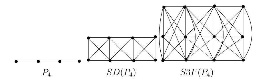
Figure 1. The strong double graph and strong 3-fold graph of \(P_4\).

p-fold graph to construct some new families of graphs G for which

\[E(G) > LE(G). (1)\]

Using singular value inequality it can be seen that for bipartite graphs the inequality \(E(G) \le LE(G)\) always holds [21]. So for the reverse inequality we will search for non-bipartite graphs. For other undefined notations and terminology from graph theory and spectral graph theory, the readers are referred to [5, 17].

Let \(KK_n^j\), \(1 \le j \le n\) be the graph defined above. The A-spectrum and L-spectrum of \(KK_n^j\) were found in [9] and are given by the following results.

Lemma 1.1. If \(1 \le j \le n\), \(n \ge 3\), the A-characteristic polynomial of \(KK_n^j\) is \((x+1)^{2n-4}h(x)\), where \(h(x) = x^4 + (4-2n)x^3 + (n^2-6n+6-j)x^2 + (2n^2-6n+2nj-j^2-3j+4)x + (1+nj^2-2j^2+n^2-2n-2j+3jn-jn^2)\).

Lemma 1.2. If \(1 \le j \le n\), \(n \ge 3\), the L-characteristic polynomial of \(KK_n^j\) is \(x(x-n)^{2n-j-2}(x-n-1)^{j-1}g(x)\), where \(g(x) = x^2 - (n+1+j)x + 2j\).

By Lemma 1.2, the L-spectrum of the graph \(KK_n^j\) is

\[\{n^{[2n-j-2]}, n+1^{[j-1]}, \frac{(n+j+1)+\sqrt{(n+j+1)^2-8j}}{2}, \frac{(n+j+1)-\sqrt{(n+j+1)^2-8j}}{2}, 0\},\\]

with average vertex degree \(n-1+\frac{j}{n}\). Therefore,

\[\begin{split} LE(KK_n^j) &= (2n-j-2)|n-n+1-\frac{j}{n}| + (j-1)|n+1-n+1-\frac{j}{n}| \\ &+ |\frac{(n+j+1)+\sqrt{(n+j+1)^2-8j}}{2} - n + 1 - \frac{j}{n}| + |0-n+1-\frac{j}{n}| \\ &+ |\frac{(n+j+1)-\sqrt{(n+j+1)^2-8j}}{2} - n + 1 - \frac{3}{n}| \\ &= 3n-j + \frac{4j}{n} - 5 + \sqrt{(n+j+1)^2-8j}. \end{split}\]

So for any j, \(1 \le j \le n\), the Laplacian energy of the graph \(KK_n^j\) is

\[LE(KK_n^j) = 3n - j + \frac{4j}{n} - 5 + \sqrt{(n+j+1)^2 - 8j}.\] (2)

It is easy to see that \(LE(KK_n^j)\) is an increasing function of \(j, 1 \le j \le n\). Therefore it follows that \(\{KK_n^j, 1 \le j \le n\}\) gives a family of graphs where adding an edge one by one, increases the Laplacian energy monotonically. So we have the following observation.

Theorem 1.1. Among the family \(\{KK_n^j, 1 \le j \le n\}\), the graph \(KK_n^1\) has the minimal Laplacian energy and the graph \(KK_n^n\) has the maximal Laplacian energy.

Two graphs \(G_1\) and \(G_2\) of same order are said to be equienergetic if \(E(G_1) = E(G_2)\) see [2]. In analogy to this two graphs \(G_1\) and \(G_2\) of same order are said to L-equienergetic if \(LE(G_1) = LE(G_2)\) see [10, 18, 19]. Since cospectral (Laplacian cospectral) graphs are always equienergetic (L-equienergetic) the problem of constructing equienergetic (L-equienergetic) graphs is only considered for non-cospectral (non-Laplacian-cospectral) graphs.

For j=n, we have \(LE(KK_n^n)=3n-n+\frac{4n}{n}-5+\sqrt{(n+n+1)^2-8n}=4n-2=LE(K_{2n})\). Since the L-spectrum of the graph \(K_{2n}\) is \(\{2n^{[2n-1]},0\}\), it follows by Lemma 1.2, these graphs are non-Laplacian cospectral. Therefore we have the following.

Theorem 1.2. For \(j \in \mathbb{N}\), \(1 \leq j \leq n\), the graphs \(KK_n^n\) and \(K_{2n}\) are non-Laplacian cospectral, Laplacian equienergetic graphs.

Let G and H be two graphs with disjoint vertex sets. Let \(u \in V(G)\) and \(v \in V(H)\). Construct the graph \(G \star H\) from copies of G and H, by identifying the vertices u and v. Thus \(|V(G \star H)| = |V(G)| + |V(H)| - 1\). The graph \(G \star H\) is known as the coalescence of G and H with respect to u and v. For \(G = K_n\), \(H = K_{n+1}\) and u (respectively v) any vertex of G (respectively H), we have \(G \star H = K_n \star K_{n+1} = KK_n^n\). So we have the following consequence.

Corollary 1.1. If \(G = K_n\) and \(H = K_{n+1}\), then

\[LE(G \star H) = LE(KK_n^n) = LE(K_{2n})\]
= \(4n - 2 = 2n - 2 + 2(n + 1) - 2 = LE(K_n) + LE(K_{n+1}).\)

From this, it follows that the Laplacian energy of the coalescence of a complete graph on n vertices with a complete graph on n+1 vertices is the sum of their Laplacian energies, which in turn is same as the Laplacian energy of the complete graph on 2n vertices.

In [22], it is shown that inequality (1) holds for the graph \(KK_n^2\). Here we first show that the inequality (1) also holds for the graphs \(KK_n^3\) and \(KK_n^4\), and using this argument, we prove a general result (Theorem 1.4), which generalizes Proposition 1 (of [22]).

Theorem 1.3. For \(n \ge 8\) and j = 3, 4, we have \(E(KK_n^j) > LE(KK_n^j)\).

Proof. For j = 3, it follows from Lemma 1.1, that the A-characteristic polynomial \(P(KK_n^3, x)\) of the graph \(KK_n^3\) is \(P(KK_n^3, x) = (x+1)^{2n-4}h(x)\), where \(h(x) = x^4 - 2(n-2)x^3 + (n^2 - 6n + 3)x^2 + (2n^2 - 14)x + (16n - 23 - 2n^2)\).

For \(n \ge 8\), we have \(h(n) = n^2 + 2n - 23 > 0\), h(n-1) = -9 < 0, \(h(n-2) = (n-1)^2 > 0\), \(h(1) = n^2 + 8n - 29 > 0\), \(h(0) = -2n^2 + 16n - 23 < 0\), \(h(-2.3) = -1.31n^2 + 8.594n + 4.3861 < 0\), \(h(-3) = n^2 + 16n + 19 > 0\).

Therefore, h(x) has three positive roots, one in each of the intervals (0,1), (n-2,n-1) and (n-1,n), and a single negative root in the interval (-3,-2.3). Assume that \(x_1,x_2,x_3,x_4\) are the roots of h(x) with \(x_1,x_2,x_3>0\) and \(x_4<0\). Therefore the A-spectrum of the graph \(KK_n^3\) is \(\{-1^{[2n-4]},x_1,x_2,x_3,x_4\}\), with \(x_1+x_2+x_3+x_4=2(n-2)\). We have

\[E(KK_n^3) = (2n-4)|-1| + |x_1| + |x_2| + |x_3| + |x_4|\] \[= 2n - 4 + x_1 + x_2 + x_3 - x_4\] \[= 2n - 4 + 2n - 4 - 2x_4\] \[> 4n - 3.4.\]

By (2), the Laplacian energy of \(KK_n^3\) is

\[LE(KK_n^3) = 3n - 8 + \frac{12}{n} + \sqrt{n^2 + 8n - 8}.\]

So \(E(KK_n^3) - LE(KK_n^3) = n + 4.6 - \frac{12}{n} - \sqrt{n^2 + 8n - 8} = g(n)\). It is easy to see that g(n) > 0 for all \(n \ge 8\). That is, \(E(KK_n^3) > LE(KK_n^3)\), for all \(n \ge 8\).

Using the same argument as above, it can be seen that for j=4, the polynomial h(x) has three positive roots, one in each of the intervals (0,1), (n-2,n-1) and (n-1,n), and a single negative root in the interval (-3,-2.4). So proceeding similarly the result follows.

Now we obtain the lower and upper bounds for the energy of \(KK_n^j\).

Theorem 1.4. For \(k \in \mathbb{N} - \{1\}\), \((k-1)^2 < j \le k^2\) and \(n \ge ((k-1)^2 + 2)^2 - (k-1)^2\), we have

\[4n - 8 + 2k < E(KK_n^j) < 4n - 8 + 2(k+1).\]

Proof. By Lemma 1.1, the A-characteristic polynomial \(P(KK_n^j, x)\) of the graph \(KK_n^j\) is

\[P(KK_n^j, x) = (x+1)^{2n-4}h(x),\]

where

\[\begin{split} h(x) &= x^4 + (4-2n)x^3 + (n^2 - 6n + 6 - j)x^2 \\ &\quad + (2n^2 - 6n + 2nj - j^2 - 3j + 4)x \\ &\quad + (1+nj^2 - 2j^2 + n^2 - 2n - 2j + 3jn - jn^2). \end{split}\]

Let x1, x2, x3, x⁴ be the zeros of the polynomial h(x). Then the spectrum of the graph KK^j n is {−1 [2n−4], x1, x2, x3, x4}.

For (k − 1)² < j ≤ k 2 and n ≥ ((k − 1)² + 2)² − (k − 1)² , we have the following.

\[h(n) = n^2 + 2n + 1 - 2j^2 - 2j > 0,\] \[h(n-1) = -j^2 < 0,\] \[h(n-2) = (n-1)^2 > 0,\] \[h(0) = 1 - 2j - 2j^2 - 2n + 3nj + nj^2 + n^2 - jn^2 < 0,\] \[h(-k) = k^4 + (2n-4)k^3 + (n^2 - 6n + 6 - j)k^2 - (2n^2 - 6n + 2nj - j^2 - 3j + 4)k\] \[+(1 + nj^2 - 2j^2 + n^2 - 2n - 2j + 3jn - jn^2) < 0,\] \[h(-(k+1)) = k^4 + 2nk^3 + (n^2 - j)k^2 + (j^2 + j - 2nj)k + (jn + nj^2 - jn^2 - j^2) > 0.\]

Therefore, by Intermediate Value Theorem, it follows that h(x) has three positive roots, one in each of the intervals (0, n−2),(n−2, n−1) and (n−1, n), and a single negative root in the interval (−(k + 1), −k). Assume that x1, x2, x³ > 0 and x⁴ < 0. Since x¹ + x² + x³ + x⁴ = 2(n − 2). We have

\[E(KK_n^j) = (2n-4)|-1| + |x_1| + |x_2| + |x_3| + |x_4|\] \[= 2n - 4 + x_1 + x_2 + x_3 - x_4\] \[= 2n - 4 + 2n - 4 - 2x_4\] \[= 4n - 8 - 2x_4.\]

The result follows from the fact that x⁴ ∈ (−(k + 1), −k) implies −(k + 1) < x⁴ < −k, which implies k < −x⁴ < k + 1.

Since (k − 1)² < j ≤ k 2 implies k − 1 < √ j < k, we have the following consequence of Theorem 1.4.

Corollary 1.2. For \[k \in \mathbb{N} - \{1\}\], \((k-1)^2 < j \le k^2\) and \(n \ge ((k-1)^2 + 2)^2 - (k-1)^2\), we have \[E(KK_n^j) > 4n - 8 + 2\sqrt{j}.\]

A graph G on n vertices is said to be hyperenergetic if its energy exceeds the energy of the complete graph Kn, that is E(G) > E(Kn) = 2(n − 1). Since KK^j n is a graph on 2n vertices, we have the following.

Corollary 1.3. For k ∈ N − {1, 2},(k − 1)² < j ≤ k ² and n ≥ ((k − 1)² + 2)² − (k − 1)² , the graph KK^j n is hyperenergetic.

Proof. Since k ≥ 3, we have by Theorem 1.4, E(KK^j n ) > 4n−8+2k ≥ 4n−2 = E(K2n).

Corollary 1.4. For \(k \in \mathbb{N} - \{1\}\), \((k-1)^2 < j \le k^2\) and \(n \ge ((k-1)^2 + 2)^2 - (k-1)^2\), we have \(E(KK_n^j) > LE(KK_n^j)\).

Proof. For k = 2, we have j = 2, 3, 4 and \(n \ge 8\), the result follows by Proposition 1 (of [22]) and Theorem 1.3. So assume that \(k \ge 3\). By equation (2) and Corollary 1.2, we have

\[E(KK_n^j) - LE(KK_n^j) = 4n - 8 + 2\sqrt{j} - 3n + j - \frac{4j}{n} + 5 - \sqrt{(n+j+1)^2 - 8j}\]\[= n + 2\sqrt{j} + j - 3 - \frac{4j}{n} - \sqrt{(n+j+1)^2 - 8j} = g(n).\]

It is easy to see that g(n) > 0, for \(n \ge ((k-1)^2 + 2)^2 - (k-1)^2, \ k \ge 3\). Therefore the result follows. \(\Box\)

By a suitable labelling of vertices, the adjacency matrix \(A = A(KK_n^j)\) of the graph \(KK_n^j\), \(1 \le j \le n\), can be put in the form

\[A = \begin{pmatrix} 0 & x_{2n-1} \\ x_{2n-1}^t & B \end{pmatrix},\]

where \(x_{2n-1}\) is a (2n-1)-vector having first (n-1+j)-entries equal to 1 and rest 0 and B is the adjacency matrix of the graph \(K_{n-1} \cup K_n\).

Let the eigenvalues of A be \(\lambda_1 \geq \lambda_2 \geq \cdots \geq \lambda_{2n-1} \geq \lambda_{2n}\). Since the spectrum of B is \(\{n-1, n-2, -1^{[2n-3]}\}\), by interlacing inequalities for principal submatrix, we have

\[\lambda_1 \ge n - 1 \ge \lambda_2 \ge n - 2 \ge \lambda_3 \ge -1 \ge \lambda_4 \ge -1 \ge \dots \ge -1 \ge \lambda_{2n-1} \ge -1 \ge \lambda_{2n}\].

From this it follows that \(\lambda_1\in(2n-1,n-1), \lambda_2\in(n-2,n-1), \lambda_3\in(-1,n-2), \lambda_{2n}\in(-1,-2n+1)\) and \(\lambda_4=\lambda_5=\dots=\lambda_{2n-1}=-1\). This shows that the eigenvalue \(\lambda_1, \ \lambda_2\) are always positive and \(\lambda_{2n}\) always negative, while as \(\lambda_3\) may be positive or negative. Also it is clear from this and Lemma 1, that \(\lambda_1, \lambda_2, \lambda_3, \lambda_{2n}\) are the zeros of the polynomial \(h(x)=h(x)=x^4+(4-2n)x^3+(n^2-6n+6-j)x^2+(2n^2-6n+2nj-j^2-3j+4)x+(1+nj^2-2j^2+n^2-2n-2j+3jn-jn^2)\). So \(\lambda_1+\lambda_2+\lambda_3+\lambda_{2n}=2n-4\) and \(\lambda_1\lambda_2\lambda_3\lambda_{2n}=1+nj^2-2j^2+n^2-2n-2j+3jn-jn^2\). Since \(\lambda_1,\lambda_2>0\) and \(\lambda_{2n}<0\), it follows that \(\lambda_3>0\) if and only if \(1+nj^2-2j^2+n^2-2n-2j+3jn-jn^2<0\), which is so if and only if \(2\leq j\leq n-3\). Therefore we have the following result.

Theorem 1.5. For \(5 \le j \le n-3\) and \(n \ge 9\), we have \(E(KK_n^j) > LE(KK_n^j)\) if and only if

\[n > \frac{j^2 - 3j + 16 + \sqrt{(j^2 - 3j + 16)^2 + 4(j - 4)(j^2 - 2j + 16)}}{2(j - 4)}.\]

Proof. Since, for \(5 \le j \le n-3\), the eigenvalue \(\lambda_3 > 0\), therefore we have

\[E(KK_n^j) = (2n - 4)|-1| + |\lambda_1| + |\lambda_2| + |\lambda_3| + |\lambda_{2n}|\] \[= 2n - 4 + \lambda_1 + \lambda_2 + \lambda_3 - \lambda_{2n}\] \[= 2n - 4 + 2n - 4 - 2\lambda_{2n}\] \[= 4n - 8 - 2\lambda_{2n}.\]

Also by Theorem 1.1, we have \(4n-4=LE(KK_n^0)< LE(KK_n^1)< LE(KK_n^1)< LE(KK_n^n)=4n-2,\) for all \(5\leq j\leq n-3.\) So instead of showing \(E(KK_n^j)> LE(KK_n^j),\) we will show \(E(KK_n^j)> LE(KK_n^n).\) We have

\[E(KK_n^j) - LE(KK_n^n) = 4n - 8 - 2\lambda_{2n} - 4n + 2\]
= -6 - 2\lambda_{2n} > 0

if and only if \(\lambda_{2n} < -3\) which, by the Intermediate Value Theorem, is equivalent to h(-3) < 0, that is \((j-4)n^2 - (j^2 - 3j + 16)n - (j^2 - 2j + 16) > 0\), that is \(n > \frac{j^2 - 3j + 16 + \sqrt{(j^2 - 3j + 16)^2 + 4(j - 4)(j^2 - 2j + 16)}}{2(j-4)}\).

The conditions of Theorem 1.5 are also sufficient for the graph \(KK_n^j\) to be hyperenergetic.

If u (respectively v) is a vertex in G (respectively H) and \(G \star H\) is their coalescence, then it is shown in [21] that

\[E(G \star H) \le E(G) + E(H),\tag{3}\]

with equality if and only if either u is an isolated vertex of G or v is an isolated vertex of H or both are isolated vertices.

For j = n, we have \(KK_n^n = K_n \star K_{n+1}\). So for \(G = K_n\) and \(H = K_{n+1}\), we have by (3)

\[E(KK_n^n) = E(K_n \star K_{n+1}) < E(K_n) + E(K_{n+1})\]
= \(2n - 2 + 2(n+1) - 2 = 4n - 2 = LE(KK_n^n)\).

From this it follows that the graph \(KK_n^n\) is not hyperenergetic.

2. On strong graphs and strong p-fold graphs

For a graph G with vertex set \(V(G) = \{v_1, v_2, \ldots, v_n\}\), the strong double graph SD(G) is a graph obtained by taking two copies of G and joining each vertex \(v_i\) in one copy with the closed neighbourhood \(N[v_i] = N(v_i) \cup \{v_i\}\) of corresponding vertex in another copy. In other words, strong double graph of the graph G with vertex set \(V(G) = \{v_1, v_2, \ldots, v_n\}\) is the graph SD(G) with vertex set \(V(SD(G)) = \{x_1, x_2, \ldots, x_n, y_1, y_2, \ldots, y_n\}\), where the adjacency is defined as follows. \(x_i(y_i)\) is adjacent to \(x_j(y_j)\) if \(v_i\) adjacent to \(v_j\); and \(x_i\) adjacent to \(y_j\) if i = j or \(v_i\) adjacent to \(v_j\) (see Figure 1).

The following observations can be found in [18].

Lemma 2.1. If \(\lambda_i\), i = 1, 2, ..., n, is the A-spectrum of the graph G, then the A-spectrum of the graph SD(G) is \(2\lambda_i + 1, -1^{[n]}\), i = 1, 2, ..., n.

Lemma 2.2. If \(\mu_i\) and \(d_i\), i = 1, 2, ..., n, are respectively the L-spectrum and degree sequence of the graph G, then the L-spectrum of the graph SD(G) is \(2\mu_i, 2d_i + 2, i = 1, 2, ..., n\).

Figure 2. Graph H is the only graph on 7 vertices with E(H) > LE(H). Graph \(G_1\) is one of the graphs with \(E(G_1) > LE(G_1)\), but \(E(SPF(G_1)) \le LE(SPF(G))\).

For the graph H (see Figure 2) it is shown in [15] that E(H) > LE(H) and using this, an infinite families of graphs (disconnected) were constructed for which the inequality (1) holds. Here we show inequality (1) also holds for SD(H). By direct calculation it can seen that the A-spectrum of H is

\[\{3.17741, 1.73205, 0.67836, 1^{[2]}, 1.73205, 1.85577\}\]

and its L-spectrum is

\[\{4+\sqrt{2},3+\sqrt{3},4^{[2]},4-\sqrt{2},3-\sqrt{3},0\}.\]

Using Lemmas 2.1 and 2.2, and the fact that the degree sequence of H is [4,3,3,3,3,3,3], it follows that the A-spectrum and L-spectrum of the graph SD(H) are respectively as

\[\{7.35482, 4.4641, 2.35672, -1^{[9]}, -2.4641, -2.71154\}\]

and

\[\{10, 8 + 2\sqrt{2}, 6 + 2\sqrt{3}, 8^{[8]}, 8 - 2\sqrt{2}, 6 - 2\sqrt{3}, 0\}.\]

Therefore LE(SD(H)) = 28.299377 < 28.3512 = E(SD(H)). That proves the assertion.

For a graph G with vertex set \(\{v_1, v_2, \dots, v_n\}\), let SPF(G) be the graph obtained by taking p-copies of the graph G and joining each vertex \(v_i\) in one copy with the closed neighbourhood \(N[v_i] = N(v_i) \cup \{v_i\}\) of the corresponding vertex in every other copy. By a suitable labelling of vertices, it can be seen that the adjacency matrix \(\widehat{A}\) of the graph SPF(G) is

\[\widehat{A} = \begin{pmatrix} A & A+I & \cdots & A+I \\ A+I & A & \cdots & A+I \\ \vdots & \vdots & \cdots & \vdots \\ A+I & A+I & \cdots & A \end{pmatrix},\]

where A is the adjacency matrix of G and I is the identity matrix of order equal to the order of A. Therefore the characteristic polynomial

On energy, Laplacian energy and p-fold graphs | H.A. Ganie, S. Pirzada, and E.T. Baskoro

\[|\lambda I_{pn} - \widehat{A}| = \begin{vmatrix} \lambda I_n - A & -(A+I) & \cdots & -(A+I) \\ -(A+I) & \lambda I_n - A & \cdots & -(A+I) \\ \vdots & \vdots & \cdots & \vdots \\ -(A+I) & -(A+I) & \cdots & \lambda I_n - A \end{vmatrix},\]

Using elementary transformations \(C_1 \to C_1 + C_2 + \cdots + C_p\) and then \(R_i \to R_i - R_1\), for \(i = 2, 3, \dots, p\), it can be seen that the spectrum of the matrix \(\widehat{A}\) and so the A-spectrum of the graph SPF(G) is

\[\{-1^{[n(p-1)]}, px_1+p-1, px_2+p-1, \dots, px_n+p-1\},\] (4)

where \(x_1, x_2, \ldots, x_n\) are the adjacency eigenvalues of the graph G.

Also the degree matrix \(\widehat{D}\) of the graph SPF(G) is

\[\widehat{D} = \begin{pmatrix} pD + (p-1)I & 0 & \cdots & 0 \\ 0 & pD + (p-1)I & \cdots & 0 \\ \vdots & \vdots & \cdots & \vdots \\ 0 & 0 & \cdots & pD + (p-1)I \end{pmatrix}.\]

So the Laplacian matrix \(\widehat{L}\) of the graph SPF(G) is

\[\widehat{L} = \begin{pmatrix} pD + (p-1)I - A & -(A+I) & \cdots & -(A+I) \\ -(A+I) & pD + (p-1)I - A & \cdots & -(A+I) \\ \vdots & \vdots & \ddots & \vdots \\ -(A+I) & -(A+I) & \cdots & pD + (p-1)I - A \end{pmatrix}.\]

Proceeding similarly as above, it can be seen that the L-spectrum of the graph SPF(G) is

\[\{p\mu_1, p\mu_2, \dots, p\mu_n, pd_1 + p^{[p-1]}, pd_2 + p^{[p-1]}, \dots, pd_n + p^{[p-1]}\},\] (5)

where \(\mu_1, \mu_2, \dots, \mu_n\) are the Laplacian eigenvalues of G and \(d_1, d_2, \dots, d_n\) are the degrees of the vertices in G.

The next result gives a two way infinite families of graphs G for which the inequality (1) holds.

Theorem 2.1. For \[j = 2, 3, 4, \ p = 2, 3 \ and \ n \ge 9 \ and for \ j = 2, 3, 4, \ p \ge 4 \ and \ n > pj\], we have \(E(SPF(KK_n^j)) > LE(SPF(KK_n^j))\).

Proof. For p=2 and j=2,3,4, we have \(SPF(KK_n^j)\cong SD(KK_n^2)\) or \(SD(KK_n^3)\) or \(SD(KK_n^3)\), respectively. If \(SPF(KK_n^j)\cong SD(KK_n^3)\), then the result follows by Theorem 4.4 in [18]. If \(SPF(KK_n^j)\cong SD(KK_n^3)\) or \(SD(KK_n^3)\), then the result follows by proceeding similarly as in Theorem 4.4 in [18]. Also for p=3 and j=2,3,4, we have \(SPF(KK_n^j)\cong KK_n^2\circ K_3\) or \(KK_n^3\circ K_3\) or \(KK_n^4\circ K_3\), respectively. Here we will show the result holds for \(SPF(KK_n^j)\cong KK_n^2\circ K_3\), and the result for the other two cases follows similarly.

The A-spectrum of the graph \(KK_n^2 \circ K_3\) is \(\{-1^{[6n-4]}, 3x_1+2, 3x_2+2, 3x_3+2, 3x_4+2\}\), where \(x_1, x_2, x_2, x_4\) are the zeros of \(h(x) = x^4 - 2(n-2)x^3 + (n^2 - 6n + 4)x^2 + 2(n^2 - n - 3)x - 2(n-2)x^3 + (n^2 - 6n + 4)x^2 + 2(n^2 - n - 3)x - 2(n-2)x^3 + (n^2 - 6n + 4)x^2 + 2(n^2 - n - 3)x - 2(n-2)x^3 + (n^2 - 6n + 4)x^2 + 2(n^2 - n - 3)x - 2(n-2)x^3 + (n^2 - 6n + 4)x^2 + 2(n^2 - n - 3)x - 2(n-2)x^3 + 2(n^2 - 6n + 4)x^2 + 2(n^2 - n - 3)x - 2(n-2)x^3 + 2(n^2 - 6n + 4)x^2 + 2(n^2 - n - 3)x - 2(n-2)x^3 + 2(n^2 - 6n + 4)x^2 + 2(n^2 - n - 3)x - 2(n-2)x^3 + 2(n^2 - 6n + 4)x^2 + 2(n^2 - n - 3)x - 2(n-2)x^3 + 2(n^2 - 6n + 4)x^2 + 2(n^2 - n - 3)x - 2(n-2)x^3 + 2(n^2 - 6n + 4)x^2 + 2(n^2 - n - 3)x - 2(n-2)x^3 + 2(n^2 - 6n + 4)x^2 + 2(n^2 - n - 3)x - 2(n-2)x^3 + 2(n^2 - 6n + 4)x^2 + 2(n^2 - n - 3)x - 2(n-2)x^3 + 2(n^2 - 6n + 4)x^2 + 2(n^2 - n - 3)x - 2(n-2)x^2 + 2(n^2 - n - 3)x - 2(n-2)x^2 + 2(n^2 - n - 3)x - 2(n-2)x^2 + 2(n^2 - n - 3)x - 2(n-2)x^2 + 2(n^2 - n - 3)x - 2(n-2)x^2 + 2(n^2 - n - 3)x - 2(n-2)x^2 + 2(n^2 - n - 3)x - 2(n-2)x^2 + 2(n^2 - n - 3)x - 2(n-2)x^2 + 2(n^2 - n - 3)x - 2(n-2)x^2 + 2(n^2 - n - 3)x - 2(n-2)x^2 + 2(n^2 - n - 3)x - 2(n-2)x^2 + 2(n^2 - n - 3)x - 2(n-2)x^2 + 2(n^2 - n - 3)x - 2(n-2)x^2 + 2(n^2 - n - 3)x - 2(n-2)x^2 + 2(n^2 - n - 3)x - 2(n-2)x^2 + 2(n^2 - n - 3)x - 2(n-2)x^2 + 2(n^2 - n - 3)x - 2(n^2 - n - 3)x - 2(n^2 - n - 3)x - 2(n^2 - n - 3)x - 2(n^2 - n - 3)x - 2(n^2 - n - 3)x - 2(n^2 - n - 3)x - 2(n^2 - n - 3)x - 2(n^2 - n - 3)x - 2(n^2 - n - 3)x - 2(n^2 - n - 3)x - 2(n^2 - n - 3)x - 2(n^2 - n - 3)x - 2(n^2 - n - 3)x - 2(n^2 - n - 3)x - 2(n^2 - n - 3)x - 2(n^2 - n - 3)x - 2(n^2 - n - 3)x - 2(n^2 - n - 3)x - 2(n^2 - n - 3)x - 2(n^2 - n - 3)x - 2(n^2 - n - 3)x - 2(n^2 - n - 3)x - 2(n^2 - n - 3)x - 2(n^2 - n - 3)x - 2(n^2 - n - 3)x - 2(n^2 - n - 3)x - 2(n^2 - n - 3)x - 2(n^2 - n - 3)x - 2(n^2 - n - 3)x - 2(n^2 - n - 3)x - 2(n^2 - n - 3)x - 2(n^2 - n - 3)x - 2(n^2 - n - 3)x - 2(n^2 - n - 3)x - 2(n^2 - n - 3)x - 2(n^2 - n - 3)x - 2(n^2 - n - 3)x - 2(n^2 - n - 3)x - 2(n^2 - n - 3)x - 2\)

\((n^2 - 8n + 11)\). Proceeding similarly as in Theorem 1.3, it can be seen that \(x_1, x_2, x_3 > 0\) and \(x_4 \in (-3, -2.2)\) for \(n \ge 9\). So, we have

\[E(KK_n^2 \circ K_3) = 12n - 6x_4 - 12 > 12n + 1.2.\]

Also the L-spectrum of the graph \(KK_n^2 \circ K_3\) is \(\{3n^{[6n-10]}, 3n+3^{[5]}, 3n+6^{[2]}, \frac{3(n+3)\pm\sqrt{n^2+6n-7}}{2}, 0\}\), with average vertex degree \(3n-1+\frac{6}{n}\). We have

\[LE(KK_n^2 \circ K_3) = 9n - 13 + \frac{24}{n} + 3\sqrt{n^2 + 6n - 7}.\]

Therefore \(E(KK_n^2 \circ K_3) - LE(KK_n^2 \circ K_3) = 3n + 14.2 - \frac{24}{n} - 3\sqrt{n^2 + 6n - 7} = g(n)\). It is easy to see that g(n) > 0, for all \(n \ge 9\).

So assume that \(p \ge 4\) and j = 2, 3, 4. Using (4) and Lemma 1.1, it follows that the A-spectrum of the graph \(SPF(KK_n^j)\) is

\[\{-1^{[2pn-4]}, px_1 + (p-1), px_2 + (p-1), px_3 + (p-1), px_4 + (p-1)\},\\]

where \(x_1, x_2, x_3, x_4\) are the zeros of the polynomial \(h(x) = x^4 - 2(n-2)x^3 + (n^2 - 6n + 6 - j)x^2 + (2n^2 - 6n + 2nj - j^2 - 3j + 4)x + (1 + nj^2 - 2j^2 + n^2 - 2n - 2j + 3nj - jn^2).\)

For n > pj, \(p \ge 4\) and j = 2, 3, 4, we have \(h(n) = n^2 + 2n - 2j^2 - 2j + 1 > 0\), \(h(n-1) = -j^2 < 0\), \(h(n-2) = (n-1)^2 > 0\), \(h(1) = 16 - 6j - 3j^2 - 16n + 5jn + nj^2 + 4n^2 - jn^2 > 0\), \(h(0) = 1 + nj^2 - 2j^2 + n^2 - 2n - 2j + 3nj - jn^2 < 0\), \(h(-3) = 16 - 2j + j^2 + 16n - 3jn + nj^2 + 4n^2 - jn^2 > 0\),

\[h(-2.j) = \begin{cases} -0.56n^2 + 4.656n + 2.3936 < 0, & \text{if } j = 2\\ -1.31n^2 + 8.594n + 4.3861 < 0, & \text{if } j = 3\\ -2.04n^2 + 14.288n + 8.0016 < 0 & \text{if } j = 4. \end{cases}\]

Therefore, h(x) has three positive roots, one in each of the intervals (0,1), (n-2,n-1) and (n-1,n), and a single negative root in the interval (-3,-2.j). Assume that \(x_1,x_2,x_3>0\) and \(x_4<0\). We have

\[E(SPF(KK_n^j)) = (2pn - 4)|-1| + |px_1 + p - 1| + |px_2 + p - 1| + |px_3 + p - 1| + |px_4 + p - 1| + |px_4 + p - 1|\] \[= 2pn - 4 + p(x_1 + x_2 + x_3) - px_4 + 2p - 2\] \[= 2pn - 4 + p(2n - 4 - x_4) - px_4 + 2p - 2\] \[= 4pn - 2p - 2px_4 - 6\] \[> 4pn + 2p(1, j) - 6.\]

Also by Lemma 1.2, equation (5) and the fact that the degree sequence of the graph \(KK_n^j\) is \([n+j-1,n^{[j]},(n-1)^{[2n-j-1]}]\), it follows that the L-spectrum of the graph \(SPF(KK_n^j)\) is

\[\{pn^{[2pn-p(j+1)-1]}, p(n+1)^{[pj-1]}, p(n+j)^{[p-1]}, \frac{p((n+j+1)\pm\sqrt{(n+j+1)^2-8j})}{2}, 0\}\]

with average vertex degree \(pn-1+\frac{pj}{n}\). Therefore, we have

\[\begin{split} LE(SPF(KK_n^j)) &= (2pn - p(j+1) - 1)|pn - pn + 1 - \frac{pj}{n}| + (pj - 1)|pn + p - pn + 1 - \frac{pj}{n}| \\ &+ (p-1)|pn + pj - pn + 1 - \frac{pj}{n}| + |0 - pn + 1 - \frac{pj}{n}| + \\ &+ |\frac{p((n+j+1) - \sqrt{(n+j+1)^2 - 8j})}{2} - pn + 1 - \frac{pj}{n}| \\ &+ |\frac{p((n+j+1) + \sqrt{(n+j+1)^2 - 8j})}{2} - pn + 1 - \frac{pj}{n}| \\ &= 3pn - p(j+1) - 4 + \frac{4pj}{n} + p\sqrt{(n+j+1)^2 - 8j}. \end{split}\]

For n > pj, \(p \ge 4\) and j = 2, 3, 4, we have \(E(SPF(KK_n^j)) - LE(SPF(KK_n^j)) = pn + p(2(1.j) + j + 1) - 2 - \frac{4pj}{n} - p\sqrt{(n+j+1)^2 - 8j} > 0\). That is, \(E(SPF(KK_n^j)) > LE(SPF(KK_n^j))\), for all n > pj, \(p \ge 4\) and j = 2, 3, 4.

Remark 2.1. From Theorems 1.3 and 2.1, one may get an insight that the inequality E(SPF(G)) > LE(SPF(G)) holds whenever the inequality E(G) > LE(G) holds. This is not always true, in fact there are graphs G for which E(G) > LE(G) hold, but E(SPF(G)) > LE(SPF(G)) does not hold. For example, consider the graph \(G_1\) as shown in Figure 2. For this graph A-spectrum is

\[\{-2.5616, -2.3444, -1.2837, -0.8643, -0.4633, 0.6766, 0.8543, 1.9383, 4.0482\}\]

and L-spectrum is

\[\{0, 1.7888, 3.1355, 3.5858, 4.1973, 4.6874, 5.3643, 6.4142, 6.8267\}.\]

So \(E(G_1) = 15.0347 > 14.9798 = LE(G_1)\). By Lemma 1.1, the A-spectrum of the graph \(SD(G_1) = S2F(G_1)\) is

\[\{-1^{[9]}, -4.1232, -3.6888, -1.5676, -0.7286, 0.0734, 2.3532, 2.7086, 4.8766, 9.0964\}.\]

Also by Lemma 1.2 and the fact the degree sequence of the graph \(G_1\) is [3, 4, 4, 4, 4, 4, 4, 4, 5], it follows that the L-spectrum of \(SD(G_1)\) is

\[\{0, 3.5776, 6.271, 7.1716, 8.3946, 9.3748, 10.7286, 12.8284, 13.6534, 8, 10^{[7]}, 12\}.\]

Therefore \[E(SD(G_1)) = 38.2162 < 41.1704 = LE(SD(G_1)).\]

Although the conjecture that "the inequality \(LE(G) \ge E(G)\) holds for all G" has been disproved. This inequality holds for most of the graphs as shown in [12] and [22]. Therefore the following problem will be of great interest.

Problem 1. Characterize all non-bipartite graphs G for which the inequality \(LE(G) \geq E(G)\) holds.

Acknowledgement

The authors wish to thank the referees for the valuable comments which improved the presentation of the paper. The third author was supported by Research Grant "Program Riset Unggulan ITB-DIKTI" 2015, Ministry of Research, Technology and Higher Education, Indonesia.

References

• [1] T. Alesic, Upper bounds for Laplacian energy of graphs, MATCH Commun. Math. Comput. Chem. 60 (2008), 435–439.
• [2] R. Balakrishnan, The energy of a graph, Linear Algebra Appl. 387 (2004), 287–295.
• [3] Z. Chen, Spectra of extended double cover graphs, Czech. Math. J. 54 (2004), 1077–1082.
• [4] T. A. Chishti, Hilal A. Ganie and S. Pirzada, Properties of strong double graphs, J. Discrete Math. Sc. and Cryptography 17(4) (2014), 311–319.
• [5] D. Cvetkovic, M. Doob and H. Sachs, Spectra of graphs-Theory and Application, Academic Press, New York, 1980.
• [6] D. Cvetkovic, S. K. Simic, Towards a spectral theory of graphs based on signless Laplacian I, Publ. Inst. Math. (Beograd) 85 (2009), 19–33.
• [7] G. H. Fath-Tabar, A. R. Ashrafi, Some remarks on the Laplacian eigenvalues and Laplacian energy of graphs, Math. Commun. 15 (2010), 443–451.
• [8] M. Fiedler, Algebraic Connectivity of Graphs, Czech. Math. J. 23 (1973), 298–305.
• [9] M. Freitas, R. Del-Vecchio, N. Abreu, Spectral properties of KK^{j n} graphs, Matematica Contemporanea 39 (2010), 129–134.
• [10] Hilal A. Ganie, S. Pirzada, Ivanyi Antal, Energy, Laplacian energy of double graphs and new families of equienergetic graphs, Acta Univ. Sap. Informatica, 6 (1) (2014), 89–116.
• [11] I. Gutman, The Energy of a graph, Ber. Math. Statist. Sekt. Forschungszenturm Graz. 103 (1978), 1–22.
• [12] I. Gutman, N. M. M. de Abreu, C. T. M. Vinagre, A. S. Bonifacio, S. Radenkovic, Relation between Energy and Laplacian Energy, MATCH Commun. Math. Comput. Chem. 59 (2008), 343–354.
• [13] I. Gutman and O. E. Polansky, Mathematical concepts in organic chemistry, Springer-Verlag, Berlin 1986.
• [14] I. Gutman and B. Zhou, Laplacian energy of a graph, Linear Algebra Appl. 414 (2006), 29– 37.

• [15] J. Liu and B. Liu, on the relation between Energy and Laplacian energy, MATCH Commun. Math. Comput. Chem. 61 (2009), 403–406.
• [16] X. Li, Y. Shi and I. Gutman, Graph Energy, Springer New York, (2012).
• [17] S. Pirzada, An Introduction to Graph Theory, Universities Press, Orient Blackswan, (2012).
• [18] S. Pirzada and Hilal Ahmad, Spectra, energy and Laplacian energy of strong double graphs, Springer Proceedings in Mathematics and Statistics, to appear.
• [19] S. Pirzada and Hilal Ahmad, On the construction of L-equienergetic graphs, submitted.
• [20] S. Radenkovic and I. Gutman, Total electron energy and Laplacian energy: How far the analog goes?, J. Serb. Chem. Soc. 72 (2007), 1343–1350.
• [21] W. So, M. Robbiano, N. M. M. de Abreu, I. Gutman, Applications of a theorem by Ky Fan in the theory of graph energy, Linear Algebra and its Applications 432 (2010) 2163–2169.
• [22] D. Stevanovic, I. Stankovic and M. Milosevic, More on the relation between Energy and Laplacian energy of graphs, MATCH Commun. Math. Comput. Chem. 61 (2009), 395–401.
• [23] H. Wang and H. Hua, Note on Laplacian energy of graphs, MATCH Commun. Math. Comput. Chem. 59 (2008), 373–380.
• [24] B. Zhou, More on energy and Laplacian energy, MATCH Commun. Math. Comput. Chem. 54 (2010), 75–84.
• [25] B. Zhou and I. Gutman, On Laplacian energy of graphs, MATCH Commun. Math. Comput. Chem. 57 (2007), 211–220.