Jeremy Moody, P.K. Aravind
Physics Department, Worcester Polytechnic Institute, Worcester, MA
moody.jeremy@gmail.com, paravind@wpi.edu
This paper shows how a method developed by Van Steenwijk can be generalized to calculate the resistance between any two vertices of a symmetrical polytope all of whose edges are identical resistors. The method is applied to a number of structures that have not been considered earlier such as the Archimedean polyhedra and their duals in three dimensions, the regular polytopes in four dimensions and the hypercube in any number of dimensions.
Keywords: Resistor networks, Electrical circuits, polyhedra, polytopes, hypercubes.
Mathematics Subject Classification : 05C90
DOI: 10.5614/ejgta.2015.3.1.7
1. Introduction
The problem of determining the equivalent resistance between arbitrary nodes of a symmetrical resistor network has received much attention over the years. Perhaps the best known instance of this problem is that of finding the resistance between opposite vertices of a cube all of whose edges are identical resistors[1]. Van Steenwijk[2] generalized this problem to that of finding the resistance between arbitrary vertices of a regular polyhedron whose edges are identical resistors. He showed how the superposition principle could be used in conjunction with the symmetries of these structures to derive a closed form expression for the resistance between any two vertices in terms of the topological characteristics of these structures. Similar problems have been solved for
Received: 05 September 2014, Revised: 20 February 2015, Accepted: 16 March 2015.
infinite networks. Many years back Purcell[3] posed the problem of finding the resistance between diagonally opposite mesh points of an infinite square lattice of identical resistors. Atkinson and Van Steenwijk[4] generalized this problem to that of finding the resistance between arbitrary nodes of a square, triangular or honeycomb lattice in two dimensions, or other types of lattices in three or more dimensions. They showed how these problems could be solved using a Fourier transform approach, whereas Cserti[5] solved the same problems using a Green's function approach. The equivalent resistance between a pair of nodes in an infinite lattice is directly related to the transition probability between these nodes under a suitably biased random walk. A nice explanation of this point is given in the book by Nahin[6], which also gives references to further literature on this topic.
The purpose of this paper is to return to the problem solved originally by Van Steenwijk[2] and generalize it in a new direction: we will calculate the resistance between arbitrary vertices of a symmetrical polytope all of whose edges are identical resistors. By a "polytope" we mean the generalization of a polygon in higher dimensions. In three dimensions a polytope is simply a polyhedron, whereas in four dimensions it is a figure whose boundary consists of polyhedra (just as the boundary of a polyhedron consists of polygons). The three types of polytopes we will consider in this paper are the following:
- (1) Semiregular polyhedra (such as the cuboctahedron) and their duals (such as the rhombic dodecahedron). The former solids are vertex-transitive and can be treated by a minor modification of Van Steenwijk's original method, but the latter solids are not because they have vertices of more than one kind. For example, a network based on the rhombic dodecahedron has nodes (or vertices) of degree four (i.e., ones where four edges meet) as well as nodes of degree three (where three edges meet). Thus one is faced with the problem of calculating the resistance between nodes of the same type as well as those of different types. Solving this problem requires an extension of Van Steenwijk's original method, but this extension makes it applicable to a significantly wider range of cases.
- (2) The regular polytopes in four dimensions, which are the analogs of the regular (or Platonic) solids in three dimensions. There are six such figures, of which the hypercube is perhaps the best known (at least in the popular youtube culture), but we will single out the more complicated 600 cell for special treatment. We do this because it provides an excellent illustration of the efficacy of Van Steenwijk's method by showing how it allows the hundreds of equations that would result from a routine application of Kirchoff's laws to be replaced by a much smaller set.
- (3) The N-dimensional hypercube (or N-cube). Many years back Huang and Tretiak[7] calculated the resistance between diametrically opposite nodes of an N-cube for N ≥ 2. Here we generalize their result by calculating the resistance between arbitrary nodes of an N-cube.
The interest of the problems we study here is largely pedagogical. They provide illustrative examples of the power of symmetry in an elementary context that students and teachers of physics or related disciplines may find helpful. Although the networks we consider are based on three- or higher-dimensional solids, they can all be realized as circuits of the same topology whose nodes correspond to the vertices of the structure and whose (identical) resistors correspond to its edges. We have actually built circuits of a few of our models and used them to verify our theoretical predictions, as we will discuss later.
The role of symmetry in facilitating the solution to this class of problems can be understood as
follows. Consider the problem of calculating the resistance between arbitrary nodes of a convex polyhedron of V vertices, E edges and F faces, all of whose edges are identical resistors. The straightforward approach would consist of sending in a current at one vertex and taking it out at another, and using Kirchoff's node and loop laws to solve for the currents through all the edges. This would require writing down V node equations (one for each of the vertices) and F loop equations (one for each of the faces). However, only V − 1 of the node equations and F − 1 of the loop equations would be independent of each other (since the sum of all the node or loop equations is a trivial identity), so the total number of independent equations is (V −1)+ (F −1) = V +F −2 = E (from Euler's theorem for polyhedra), which is the same as the number of currents that must be solved for. The drawback of this approach is that it requires one to write down as many as V + F equations in order to solve for the generally much smaller number of distinct currents. Symmetry simplifies the task by allowing us to write down a relatively small number of equations for a minimal set of currents from which the equivalent resistance between any two nodes can be calculated by a judicious use of the principle of superposition. The exact manner in which this can be done will be explained in the next two sections, following which we turn to a discussion of the three types of polytope networks mentioned above.
2. Van Steenwijk's method
Consider a network based on a polytope of V vertices and E edges. The network has V nodes, corresponding to the vertices of the polytope, and E identical resistors (which we will take to have resistance R), corresponding to its edges. We can calculate the resistance between any two nodes of the network (the "input" and "output" nodes) using the following procedure:
(a) We feed a current I into the input node, take equal currents I/(V −1) out of all the other nodes, and solve for the currents through all the edges (using symmetry to simplify the task, in the manner we will explain in the next section). See Fig.1(a) for a diagram of this situation. Let S and T be the input and output nodes, and let n1, n2, . . . , nd be any sequence of nodes leading from S to T. Let Cab be the current flowing from node a to node b in Fig.1(a). Since each edge of the network has resistance R, the potential difference between nodes S and T in Fig.1(a) is
\[(C_{S,n_1} + C_{n_1,n_2} + \dots + C_{n_d,T})R.\] (1)
(b) Next we take a current I out of the output node after feeding equal currents of I/(V − 1) into each of the other nodes (see Fig.1(b)). The potential difference between nodes S and T is then the same as in Fig.1(a), and is given by (1). The reason for this is as follows: if all the nodes are equivalent under symmetry, and the directions of all currents are reversed in Fig.1(b), the potential difference between T and S would be the same as that between S and T in Fig.1(a); however, because the currents flow as they do, the potential difference between T and S in Fig.1(b) is the same as that between T and S in Fig.1(a).
(c) Finally we superpose the situations in Figs.1(a) and (b) so that equal currents of I+I/(V −1) = IV/(V − 1) enter and exit at the input and output nodes and no currents enter or exit at any of the other nodes (see Fig.1(c)). This is the situation of interest, and if we can calculate the potential difference between S and T, we can divide it by the external current (= IV/(V − 1)) to find
Figure 1: Calculation of the resistance between two nodes of a circuit by the principle of superposition. (a) A current I is fed in at the input node S and currents of I/(V − 1) are taken out at all the other nodes, including the output node T, (b) a current I is taken out at the output node T after currents of I/(V − 1) are fed in at all the other nodes, including the input node S, and (c) the situations in (a) and (b) are superposed to give a current of I + I/(V − 1) = IV/(V − 1) entering at the input node S and also leaving at the output node T, with no currents entering or leaving at any of the other nodes.
the equivalent resistance, Req, between S and T. However, by the principle of superposition, the potential difference between S and T in Fig.1(c) is the sum of the potential differences between these nodes in Figs.1(a) and (b), which we know to be twice the value in (1). Thus we can calculate Req from the equation
\[2(C_{S,n_1} + C_{n_1,n_2} + \dots + C_{n_d,T})R = \frac{IV}{V-1}R_{eq}.\] (2)
For a circuit in which all the nodes are equivalent under symmetry, it suffices to calculate the currents Ca,b in Fig.1(a) and then use these currents in (2) to calculate the equivalent resistance between any two nodes. This is essentially the method Van Steenwijk used to calculate resistances in the Platonic solids. Van Steenwijk actually simplified (2) further by expressing the sum of the currents on the left as the product of I and a number determined entirely by the topological characteristics of each Platonic solid. However we will stay with the form (2), because it is a convenient starting point for the calculations we will carry out in the rest of this paper.
3. Rhombic dodecahedron
To complete the discussion of the previous section, we must show how the currents through all the resistors of the network in Fig.1(a) can be calculated. At the same time we do this, we will indicate how the treatment of the previous section can be modified to make it apply to a network in which the nodes are not all identical but can be of two or more different kinds. The rhombic dodecahedron is an example of a figure that gives rise to a network with nodes of more than one
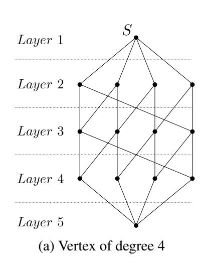
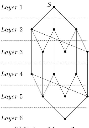
(b) Vertex of degree 3
Figure 2: Layer diagram of a rhombic dodecahedron, beginning and ending at (a) a vertex of degree 4 and (b) a vertex of degree 3. There are five layers in (a) and six layers in (b).
kind, and we will use it to illustrate how one should proceed in this more general case. The rhombic dodecahedron has 14 vertices and 24 edges, but its vertices are of two kinds: six of them are of degree four and the other eight are of degree three. The network based on it has 14 nodes and 24 resistors (all of which we take to have resistance unity). In calculating the currents in this network, it is helpful to separate the nodes into layers in the manner we now explain.
Any network has an automorphism group that consists of all the one-to-one mappings of its nodes onto themselves that preserve the edge relations in the network. In other words, if an element of the automorphism group maps the nodes Ni and Nj into N0 i and N0 j , respectively, then N0 i and N0 j are connected by an edge if and only if Ni and Nj are. It is possible to partition the nodes of a network into layers with reference to a node S; two nodes Na and Nb are defined to be in the same layer if and only if there is at least one element of the network's automorphism group that keeps S invariant but maps Na into Nb. Figures 2(a) and 2(b) show two alternative layer decompositions of a rhombic dodecahedron, the first starting at a node of degree four and the second at one of degree three. We would like to consider each of these figures in turn and see how one can determine the currents through all the edges when a current I is fed into the top node, which plays the role of the input node S in Fig.1(a), and equal currents of I/(V − 1) = I/13 are taken out at all the other nodes.
In proceeding with this task it is helpful to introduce a "layer matrix" that captures the essential features of the layers into which a network can be decomposed. For a network that has been decomposed into n layers, we define the layer matrix as a n × n matrix whose ij-th element is the number of edges going from any node in the i-th layer to nodes in the j-th layer (any node will do, since all the nodes in a layer are equivalent under symmetry). The layer matrix corresponding to
the network of Fig.2(a) is
\[L = \begin{bmatrix} 0 & 4 & 0 & 0 & 0 \\ 1 & 0 & 2 & 0 & 0 \\ 0 & 2 & 0 & 2 & 0 \\ 0 & 0 & 2 & 0 & 1 \\ 0 & 0 & 0 & 4 & 0 \end{bmatrix}\] (3)
The diagonal elements are all zero because there are no edges between nodes in the same layer. Also, the i-th row is the same as the (n+1-i)-th row written backwards, because of the inversion symmetry of the dodecahedron. Associated with any layer matrix is a current matrix C that describes the currents flowing in the network when a current I is fed in at the top node and equal currents, adding up to I, are taken out at all the other nodes. The element \(C_{ij}\) of the current matrix is the current flowing from any node in the i-th layer to any node in the j-th layer to which it is connected by an edge. The current matrix is an antisymmetric matrix because (a) the current flowing from j to i is obviously the negative of the current from i to j, and (b) there can be no current flow between nodes in the same layer (even if connecting edges do exist) because all the nodes in a layer are at the same potential.
With the layer and current matrices in hand, we can turn to the task of determining the currents in Fig.2(a) when a current of I is fed in at the top node and equal currents of I/13 are taken out at all the other nodes. Symmetry simplifies the task by allowing us to write down just one node equation for each layer and to supplement these by the few loop equations needed to determine the currents uniquely. The layer and current matrices facilitate the task of writing down the independent node equations, which follow on equating the diagonal elements of the product matrix LC with the elements of the column vector K whose first component is -I and whose remaining components are I/(V-1), where V is the number of nodes in the network. In other words, the node equations are given by
\[[LC]_{ii} = K_i \qquad (i = 1, \cdots, n) , \qquad (4)\]
where n is the number of layers in the network. On using (3) and the appropriate expressions for C and K in (4) we find that the node equations for the network of Fig.2(a) are
\[-4C_{12} = -I (5)\]
\[C_{12} - 2C_{23} = I/13 (6)\]
\[2C_{23} - 2C_{34} = I/13 \tag{7}\]
\[2C_{34} - C_{45} = I/13 (8)\]
\[4C_{45} = I/13\] . (9)
These equations have the unique solution
\[C_{12} = \frac{1}{4}I\], \(C_{23} = \frac{9}{104}I\), \(C_{34} = \frac{5}{104}I\) and \(C_{45} = \frac{1}{52}I\). (10)
We turn next to Fig.2(b) and solve for the currents when a current I is fed in at the top node and equal currents of I/13 are taken out at all the other nodes. The layer matrix is now the \(6 \times 6\)
matrix
\[L' = \begin{bmatrix} 0 & 3 & 0 & 0 & 0 & 0 \\ 1 & 0 & 2 & 1 & 0 & 0 \\ 0 & 2 & 0 & 0 & 1 & 0 \\ 0 & 1 & 0 & 0 & 2 & 0 \\ 0 & 0 & 1 & 2 & 0 & 1 \\ 0 & 0 & 0 & 0 & 3 & 0 \end{bmatrix}\] (11)
The node equations are given by \([L'C']_{ii} = K'_i\) for \(i = 1, \dots, 6\), where C' is the \(6 \times 6\) antisymmetric current matrix and K' is the 6-component vector whose first component is -I and whose remaining components are I/13. The explicit form of the node equations is
\[-3C_{12}' = -I (12)\]
\[C'_{12} - 2C'_{23} - C'_{24} = I/13 (13)\]
\[2C_{23}' - C_{35}' = I/13 (14)\]
\[C'_{24} - 2C'_{45} = I/13 \tag{15}\]
\[3C_{56}' = I/13\] (16)
These are five independent equations for six currents, and we need an additional equation to solve for the currents. The single loop equation needed for this purpose can be picked out from an inspection of Fig.2(b). One sees that one can get from the second to the fifth layer either via the third layer or the fourth layer; since the potential drops along these alternative paths must be the same, we get the loop equation
\[C'_{23} + C'_{35} - C'_{24} - C'_{45} = 0 . (17)\]
Equations (12)-(17) have the unique solution
\[C'_{12} = \frac{1}{3}I\], \(C'_{23} = \frac{11}{156}I\), \(C'_{24} = \frac{3}{26}I\), \(C'_{35} = \frac{5}{78}I\), \(C'_{45} = \frac{1}{52}I\) and \(C'_{56} = \frac{1}{39}I\). (18)
We are finally in a position to calculate the resistance between arbitrary nodes of a rhombic dodecahedron whose edges are unit resistors . Let \(R_k^{d_1d_2}\) denote the resistance between a node of degree \(d_1\) and one of degree \(d_2\) that are k edges apart. We first calculate the resistances \(R_2^{44}\) and \(R_4^{44}\) between nodes of degree 4 by using V=14, R=1 and (10) in (2) to get
\[R_2^{44} = \frac{26}{14I}(C_{12} + C_{23}) = \frac{5}{8}\] (19)
\[R_4^{44} = \frac{26}{14I}(C_{12} + C_{23} + C_{34} + C_{45}) = \frac{3}{4} . {(20)}\]
Next we calculate the resistances between nodes of degree 3 by using \(V=14,\,R=1\) and (18) in (2) to get
\[R_{2a}^{33} = \frac{26}{14I}(C'_{12} + C'_{23}) = \frac{3}{4}\] (21)
\[R_{2b}^{33} = \frac{26}{14I}(C'_{12} + C'_{24}) = \frac{5}{6}\] (22)
\[R_4^{33} = \frac{26}{14I} (C'_{12} + C'_{23} + C'_{35} + C'_{56}) = \frac{11}{12} . {23}\]
The subscripts 2a and 2b have been used in (21) and (22) to distinguish two types of nodes that are two edges apart; the former refers to nodes that are two layers apart and the latter to nodes that are three layers apart. Lastly, we calculate the hybrid resistances between a node of degree 3 and one of degree 4. We can do this by superposing the following two situations: (a) we feed a current I into a node of degree 3 and take equal currents, adding up to I, out at all the other nodes, and (b) we take a current of I out of a node of degree 4 after feeding in equal currents, adding up to I, at all the other nodes. Using V = 14, R = 1, (10) and (18) in the appropriately modified form of (2) allows us to calculate the hybrid resistances as
\[R_1^{34} = \frac{13}{14I}(C_{12} + C'_{12}) = \frac{13}{24}\] (24)
\[R_3^{34} = \frac{13}{14I}(C_{12} + C_{23} + C_{34} + C_{12}' + C_{23}' + C_{35}' = \frac{19}{24}\] (25)
To summarize, we have found the seven different resistances between the nodes of a rhombic dodecahedron given in Eqs.(19)-(25).
A similar technique can be used to analyze networks based on any of the semiregular (or Archimedean) solids or their duals (the Catalan solids). The Archimedeans have nodes of just one kind, but the Catalans have nodes of two or three different kinds. An example of a more complicated network than the one treated here is provided by the rhombic triacontahedron, which has 32 nodes and 60 edges, with 12 of the nodes being of degree 5 and the other 20 of degree 3. There are 12 different resistances between the nodes (five between nodes of degree 3, three between nodes of degree 5 and four between nodes of different degrees). The reader is invited to calculate the resistances and check his/her answers against those given in[8], where results for a number of other structures can also be found. We have restricted our analysis to the case in which all the resistors in the network are identical. If resistors of several different values are allowed, the symmetry of the network gets reduced and the number of layers in it rises, and at some point a brute force solution of all the node and loop equations might be the simplest option.
4. 600-cell
The 600-cell is one of the six four-dimensional regular polytopes. An extensive account of it, and the other regular polytopes, can be found in the classic monograph by Coxeter[9]. The 600-cell has 120 vertices and 720 edges, with 12 edges meeting at each vertex. We will calculate all the distinct resistances between vertices of the 600-cell, taking its edges to be unit resistors.
The 600-cell is vertex-transitive, and so its layer decomposition relative to any node (or vertex) is the same. From the coordinates of the vertices of the 600-cell given by Coxeter[9], one can work out how its nodes fall into layers. If one starts from any node, one finds that there are nine layers consisting of 1,12,20,12,30,12,20,12 and 1 nodes, respectively, with the layers being symmetrical about the central layer (as a consequence of the inversion symmetry of the 600-cell) and with the lone node in the last layer being the antipode of the starting node. By examining the edges of the
600-cell one can work out its \(9 \times 9\) layer matrix as
\[L = \begin{bmatrix} 0 & 12 & 0 & 0 & 0 & 0 & 0 & 0 & 0 \\ 1 & 5 & 5 & 1 & 0 & 0 & 0 & 0 & 0 & 0 \\ 0 & 3 & 3 & 3 & 3 & 0 & 0 & 0 & 0 & 0 \\ 0 & 1 & 5 & 0 & 5 & 1 & 0 & 0 & 0 & 0 \\ 0 & 0 & 2 & 2 & 4 & 2 & 2 & 0 & 0 & 0 \\ 0 & 0 & 0 & 1 & 5 & 0 & 5 & 1 & 0 & 0 \\ 0 & 0 & 0 & 0 & 3 & 3 & 3 & 3 & 0 & 0 \\ 0 & 0 & 0 & 0 & 0 & 1 & 5 & 5 & 1 & 0 \\ 0 & 0 & 0 & 0 & 0 & 0 & 0 & 12 & 0 & 0 \end{bmatrix}\] \[(26)\]
If a unit current is fed into the top node and equal currents are taken out at all the other nodes, the node equations can be obtained from (4) by using (26) for L, a \(9 \times 9\) antisymmetric matrix for C and a 9-component column vector for K whose first component 1 and whose remaining components are -1/119. This leads to the 9 node equations
\[-12C_{12} = -1 (27)\]
\[C_{12} - 5C_{23} - C_{24} = 1/119 (28)\]
\[3C_{23} - 3C_{34} - 3C_{35} = 1/119 (29)\]
\[C_{24} + 5C_{34} - 5C_{45} - C_{46} = 1/119 (30)\]
\[2C_{35} + 2C_{45} - 2C_{56} - 2C_{57} = 1/119 (31)\]
\[C_{46} + 5C_{56} - 5C_{67} - C_{68} = 1/119 (32)\]
\[3C_{57} + 3C_{67} - 3C_{78} = 1/119 (33)\]
\[C_{68} + 5C_{78} - C_{89} = 1/119 (34)\]
\[12C_{89} = 1/119 (35)\]
Only eight of these equations are independent of each other and they contain 13 unknown currents, so we must supplement them by five independent loop equations to solve uniquely for all the currents. The loop equations can be picked out from an inspection of the layer matrix (26). As one example, one sees that one can get from layer 4 to layer 6 either directly or via layer 5; since the potential drop along these alternative paths must be the same, we have the loop equation \(C_{45} + C_{56} = C_{46}\). Proceeding in a similar manner allows us to set up the five independent loop equations
\[C_{23} + C_{34} = C_{24} (36)\]
\[C_{34} + C_{45} = C_{35} (37)\]
\[C_{34} + C_{46} = C_{35} + C_{56} \tag{38}\]
\[C_{45} + C_{57} = C_{46} + C_{67} \tag{39}\]
\[C_{56} + C_{68} = C_{57} + C_{78} {.} {40}\]
Equations (27)-(40) can be solved with the aid of Maple to give
\[C_{12} = \frac{1}{12}, \quad C_{23} = \frac{899}{74970}, \quad C_{24} = \frac{449}{29988}, \quad C_{34} = \frac{149}{49980}\] (41)
\[C_{35} = \frac{19}{3060}, \quad C_{45} = \frac{121}{37485}, \quad C_{46} = \frac{40}{7497}, \quad C_{56} = \frac{79}{37485}\] (42)
\[C_{57} = \frac{67}{21420}, \quad C_{67} = \frac{1}{980}, \quad C_{68} = \frac{71}{29988}, \quad C_{78} = \frac{101}{74970}, \quad C_{89} = \frac{1}{1428} \quad .\] (43)
The resistance Rk between two nodes k edges apart can now be calculated by taking R = I = 1 and V = 120 in (2) and summing the currents over any connected set of k edges leading from the top node to a node in the k-th layer. In this way we find the eight distinct resistances
\[R_1 = \frac{119}{720}, \quad R_2 = \frac{14293}{75600}, \quad R_3 = \frac{737}{3780}, \quad R_4 = \frac{1903}{9450}\] (44)
\[R_5 = \frac{37}{180}, \quad R_6 = \frac{5231}{25200}, \quad R_7 = \frac{3179}{15120}, \quad R_8 = \frac{40}{189} \quad .\] (45)
This completes the solution to the problem. It is worth pointing out the reduction in the size of the problem made possible by the use of symmetry. For a network based on a four-dimensional convex polytope of V vertices, E edges, F faces and C cells, a straightforward application of Kirchoff's laws would lead to V node equations and F loop equations. However only V − 1 of the node equations are independent (since their sum gives the trivial identity 0 = 0) while the loop equations are subject to C − 1 constraints, so the total number of independent equations is V − 1 + F − (C − 1) = V + F − C = E (by Euler's theorem in four dimensions), which is the same as the number of currents that must be solved for. For the 600-cell, this straightforward approach would lead to 120 node equations and 1200 loop equations, from which a smaller set of 720 independent equations could be obtained to solve for all the currents. By contrast, the symmetry-based approach requires us to write down just 9 node equations (one for each layer of the network) and supplement them by 5 loop equations to solve for all the distinct currents in the problem. A four-dimensional polytope that poses an even more severe challenge than the 600-cell is the 120-cell, which has 600 vertices and 1200 edges, with 4 edges meeting at each vertex. The layer matrix is a 45 x 45 matrix, but again there is symmetry about the central layer and the only nonvanishing elements lie on a few stripes bordering the principal diagonal. Remarkably, it is possible to obtain an analytical solution for all the distinct resistances in the system; the details can be found in[8].
5. N-dimensional Hypercube
An N-dimensional hypercube has 2 N vertices and N · 2 N−1 edges, with N edges meeting at each vertex. We wish to calculate the resistance between any pair of vertices (nodes) if each edge is a unit resistor. If we arrange the nodes in layers beginning from an arbitrary node, the number of nodes in the k-th layer is ( N k−1 ) = N! (k−1)!(N−k+1)! , for 1 ≤ k ≤ N + 1. Any node in the k-th layer is connected to k − 1 nodes in the (k − 1)-th layer and N − k + 1 nodes in the (k + 1)-th layer (to see this, take the vertices of the hypercube to be (±1, ±1, · · · , ±1); then, if the starting node
is taken to be (1, 1, · · · , 1), the nodes in the k-th layer are all those having (k − 1) −1's among their coordinates, which is just the expression given). The layer matrix is thus a banded matrix whose only non-zero entries occur on the two stripes bordering the principal diagonal. Suppose a unit current is fed in at the top node and equal currents are taken out at all the other nodes. If Ck denotes the current flowing from a node in the k-th layer to a node in the (k + 1)-th layer, it is easy to see, from the banded structure of the layer matrix, that these currents obey the recursion relation
\[C_k = \frac{1}{N-k+1} \left[ (k-1)C_{k-1} - \frac{1}{2^N - 1} \right] , \qquad (46)\]
with the initial condition C1 = 1/N. If one puts the currents obtained from (46) into (2), along with I = R = 1 and V = 2N , one can get an expression for the resistance RN m between two nodes of an N-cube that are m edges apart as
\[R_m^N = 2\left[\frac{2^N - 1}{2^N}\right] \sum_{k=1}^m C_k \ , \quad 1 \le m \le N \ . \tag{47}\]
Table 1 shows the values of RN m computed from (46) and (47) for 1 ≤ m ≤ N and 1 ≤ N ≤ 9. The diagonal entries in this table (the ones with m = N) agree with the results of Tretiak and Huang[7].
| m/N | 1 | 2 | 3 | 4 | 5 | 6 | 7 | 8 | 9 |
|---|---|---|---|---|---|---|---|---|---|
| 1 | 1 | 3 4 | 7 12 | 15 32 | 31 80 | 21 64 | 127 448 | 255 1024 | 511 2304 |
| 2 | 1 | 3 4 | 7 12 | 15 32 | 31 80 | 21 64 | 127 448 | 255 1024 | |
| 3 | 5 6 | 61 96 | 241 480 | 131 320 | 12 35 | 2105 7168 | 16531 64512 | ||
| 4 | 2 3 | 25 48 | 101 240 | 7 20 | 167 560 | 929 3584 | |||
| 5 | 8 15 | 137 320 | 2381 6720 | 10781 35840 | 42061 161280 | ||||
| 6 | 13 30 | 343 960 | 2033 6720 | 9383 35840 | |||||
| 7 | 151 420 | 32663 107520 | 84677 322560 | ||||||
| 8 | 32 105 | 2357 8960 | |||||||
| 9 | 83 315 |
Table 1: The resistance RN m between two vertices of an N-dimensional hypercube m edges apart, for the values of N indicated at the tops of the columns and values of m indicated to the left of the rows. The edges of the hypercube are taken to be unit resistors.
6. Conclusion
We have shown how Van Steenwijk's method[2], suitably generalized, can be used to calculate the equivalent resistances between arbitrary nodes of a variety of finite networks based on symmetrical polytopes in three or more dimensions. The problems we have discussed, as well as their
solutions, are of an elementary nature, and so may be suitable for inclusion as enrichment material in a course on circuits, linear algebra or graph theory aimed at students from a variety of backgrounds. We would also like to suggest two project activities based on this work. The first is to build circuits of the models studied and carry out measurements on them to check the theoretical predictions. We have actually done this for a few of our models. Figure 3 shows a picture of a printed circuit board (PCB) of a network based on the four-dimensional hypercube. Each row of dots represents a vertex of the hypercube, with copper traces (of essentially zero resistance) connecting the dots and ensuring that they function as a single node. Equal resistors connecting the dots in different rows simulate the edges of the hypercube (the resistors are on the backside of the PCB and so not visible in the picture). An ohmmeter can be connected between any pair of dots in different rows to measure the resistance between the corresponding nodes. We used high precision 1 kΩ resistors for the edges of the hypercube and found that the agreement between the measured and predicted values of the resistances was much better than one percent. A software program like Spice can of course be used to simulate these circuits, but we feel that actually building and testing them might be more instructive (and enjoyable). The second activity we would like to suggest is using Monte-Carlo simulations to determine the resistances in these networks. Nahin's book[6] gives a detailed account of how this can be done, using some simple test cases for illustration. Physical models of some of our networks (such as the 600- or the 6-d hypercube) might be difficult to construct, so simulation might offer the best route to verifying the theoretical predictions in such cases.
Endnote
This paper is based on a Major Qualifying Project done by the first author, under the guidance of the second, in partial fulfillment of the requirements for a B.S. degree at Worcester Polytechnic Institute. The authors would like to thank Professor Brigitte Servatius of the Mathematics Department for helpful discussions on the theoretical aspects of the project and Professor Steven Bitar of the Electrical and Computer Engineering Department for his help in fabricating the printed circuit boards that we used to test our theoretical predictions.
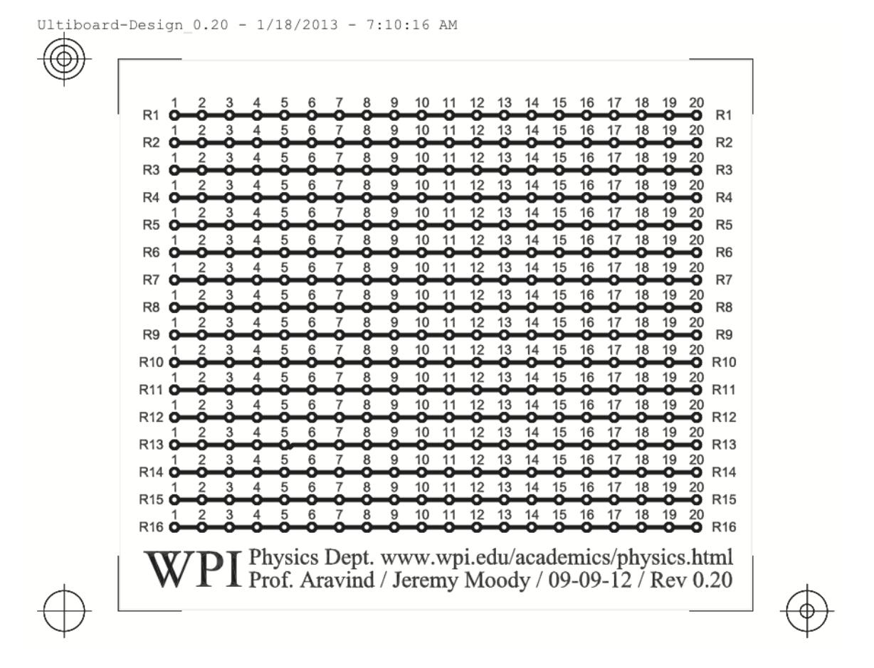
Figure 3: Printed circuit board (PCB) of a network based on a 4-dimensional hypercube. Each row of dots represents a node of the hypercube and resistances connecting the dots in different rows (on the back of the PCB and so not visible in this image) represent the edges of the hypercube.
References
- [1] See, for example, H.D.Young and R.A.Freedman, University Physics, 13th Ed (Addison-Wesley, 2012), Ch.26, Problem 92.
- [2] F.J. van Steenwijk "Equivalent resistors of polyhedral resistive structures" Am. J. Phys. 66 (1998), 90–91.
- [3] E. M. Purcell, Electricity and Magnetism, 1st Ed (McGraw-Hill, New York, 1965), p. 423.
- [4] D.Atkinson and F.J. van Steenwijk, "Infinite resistive lattices", Am. J. Phys. 67 (1999), 486– 492.
- [5] J.Cserti, "Application of the lattice Greens function for calculating the resistance of an infinite network of resistors", Am. J. Phys. 68, (2000), 896–906.
- [6] P.J.Nahin, Mrs.Perkins Electric Quilt (Princeton University Press, 2009), Chs.17 and 19 and references therein.
- [7] O.J.Tretiak and T.S.Huang, "Resistance of an N-dimensional Cube", Proc. IEEE, (1965), 1271–1272.
- [8] J.Moody, "Efficient methods for calculating equivalent resistance between nodes of a highly symmetric resistor network", A Major Qualifying Project submitted to Worcester Polytechnic Institute, E-project-032913-185209 (2013).
- [9] H.S.M.Coxeter, Regular Polytopes (Dover, New York, 1973).