Antoon H. Boodea,c, Hajo Broersma^b , Jan F. Broenink^a

^aRobotics and Mechatronics,

Faculty EEMCS, University of Twente

The Netherlands

^bFormal Methods and Tools,

Faculty EEMCS, University of Twente

The Netherlands

^cDepartment of Computer Engineering,

InHolland University of Applied Science

The Netherlands

a.h.boode@utwente.nl, h.j.broersma@utwente.nl, j.f.broenink@utwente.nl

In this paper we introduce and study a directed tree problem motivated by a new graph product that we have recently introduced and analysed in two conference contributions in the context of periodic real-time processes. While the two conference papers were focussing more on the applications, here we mainly deal with the graph theoretical and computational complexity issues. We show that the directed tree problem is NP-complete and present and compare several heuristics for this problem.

Keywords: finite deterministic directed acyclic labelled multi-graphs, vertex removing synchronised graph product, target trees, periodic real-time systems

Mathematics Subject Classification : 68R10

DOI: 10.5614/ejgta.2015.3.2.5

Received: 24 April 2015, Revised: 12 July 2015, Accepted: 22 July 2015.

1. Introduction

In this paper we give a detailed discussion of a new graph product that we have recently introduced and analysed in two conference contributions [3, 4]. While the two conference papers were focussing more on the applications, here we mainly deal with the graph theoretical and computational complexity issues.

Here we also introduce a new decision problem on directed trees. It is motivated by the applications from the context of periodic real-time processes, and it is based on the new graph product. However, this tree problem can be based on any graph product (or, in fact on any binary operation). Therefore we introduce it now, before going into the technical details of the particular application that motivated it.

1.1. A directed tree problem

Let T be a tree, so a connected acyclic (undirected) graph. We orient the tree by replacing each of the edges of T by an arc, in precisely one of the two directions, so we obtain an acyclic weakly connected directed graph, which we call a ditree. A source in a ditree is a vertex with in-degree 0. This is usually referred to as a leaf. A sink in a ditree is a vertex with out-degree 0. We call such a vertex a target of the ditree. We say that a ditree D is a target tree if D has the following properties. Each vertex except for the leaves has in-degree 2; each vertex except for one has out-degree 1; the unique vertex of D (if D has more than one vertex) with in-degree 2 and out-degree 0 is called the target of D.

In our later application, the target v of a target tree D will be interpreted as a special product of two graphs (to be defined in the sequel) that are represented by the two in-neighbours u and w of v in D. If u is a target vertex of D v, then analogously u can be interpreted as the product of two graphs, etc. On the other hand, each of the ways to compute the product of the graphs G1, . . . , Gⁿ can be represented as a target tree on n leaves and n 1 internal vertices (non-leaves). As an example, in Figure 1 we depicted a target tree corresponding to a solution of one of the heuristics called MNSA in the sequel. The leaves at the top represent graphs corresponding to processes, and the internal vertices represent products, e.g., the internal vertex numbered 1 represents the product of G¹⁶ and G2, the vertex numbered 8 represents the product of this new graph with G1, etc., and the vertex numbered 15 represents the product of the graphs represented by the vertices numbered 14 and 13, respectively. For the MNSA heuristic the order in which the products of the graphs are calculated are given by the numbers of the internal vertices. So the vertex numbered 1 represents the first product, the vertex numbered 2 represents the second product, and so on.

Figure 1. Target tree representing a solution of the MNSA heuristic.

In the sequel we will introduce two graph parameters ` and M that represent the processing time and memory occupancy of the graph corresponding to (the execution of) a process, and we will define how to compute the value of these parameters for the product of two graphs. As we will see, for the product of two graphs G<sup>1</sup> and G2, the `-value is usually lower than the sum of the two `-values of G¹ and G² (if the corresponding processes synchronise on certain actions), whereas the M-value of the product is usually larger than the sum of the two M-values. If for the execution of a number of processes on one processor we have a limited memory capacity and a deadline to make, this leads to a decision problem: can we combine the processes in such a way that we can execute them on the processor, meeting the deadline and memory restrictions?

Turning back to the target tree representation, every leaf and every internal vertex of the target tree has an associated `-value and M-value, and corresponds to one process (the leaves) or a subset (product) of more than one process (the internal vertices). Each combination of all the processes into several subsets (products) in which each process occurs in precisely one subset, is represented by a number of leaves (possibly zero) and a number of internal vertices (possibly zero), so that all the chosen vertices of the target tree cover all the leaves. Here a chosen vertex v of the target tree is said to cover all the vertices in all the directed paths from the leaves terminating in v (i.e., v covers all vertices in the (sub)ditree with target vertex v that results after deleting the arc which is directed away from v). We call a set of vertices that covers all the leaves of a target tree D precisely once a leaf cover of D. As an example, the target vertex is a leaf cover of cardinality 1 and the set of leaves is a leaf cover of cardinality n. Every leaf cover also has an associated `-value and M-value (given by the combination of processes it represents, in a way we will explain later). We say that a target tree D on n leaves is feasible if it admits a leaf cover for which the associated `-value and M-value are within the deadline and memory restrictions, so the corresponding combination of processes (corresponding to the sets of products of the graphs G1, . . . , Gⁿ associated with the n leaves) can be executed correctly on the processor. The above question translates into the following decision problem: given n graphs G1, . . . , Gⁿ (representing n processes), can we construct a feasible target tree D on n leaves (representing the graphs)? We call this the Synchronised Product Decision Problem. We will show that this decision problem is NP-complete. In fact, for obvious reasons, we will also be interested in a solution, so a target tree together with a leaf cover that provides a YES answer. If the leaf cover contains more than one vertex (so if it is not the target vertex of the target tree), the solution in fact corresponds to a forest of target trees for mutually disjoint subsets

of the n leaves.

1.2. General introduction

We continue with a general introduction that also contains the motivation for introducing the new graph product.

The software of applications of embedded control systems is often designed using a General Purpose Computing System (GPCS). Such a GPCS often has more processing power and memory available than the embedded control system. The embedded control system is the target system on which the software will run. The hardware of the target system can be very limited with respect to available memory and processing power. If such a target system has to be periodic hard real-time, it has deadlines D for its processes to fulfil the timing requirements, together with memory M to store the data of these processes.

Periodic real-time robotic applications can be designed using formal methods like process algebras [8, 9]. While designing, the designer distributes the required behaviour over up to several hundreds of processes. These processes very often synchronise over actions, e.g. to assert that a set of processes will be ready to start executing at the same time. Due to this synchronisation the application suffers from a considerable overhead related to extra context switches.

In [4] we have defined periodic real-time processes as finite deterministic directed acyclic labelled multi-graphs, where these graphs are closely related to state transition systems. The (labelled) arcs in such a graph represent actions in a periodic real-time process. The label represents the name of the action and its duration. As, per action, there is a context switch, the longest path in such a graph is the most time consuming with respect to the context switch and therefore the worst case. We introduced in [4] a Vertex-Removing Synchronised Product (VRSP) to reduce the number of context switches. VRSP is based on the synchronised product of Wohrle and Thomas [10], ¨ which is used in model-checking synchronised products of infinite transition systems.

The VRSP reduces the number of context switches and realises a performance gain for periodic real-time applications. This is achieved by (repetitively) combining two graphs representing two processes that synchronise over some action. This combined graph represents a process that will have only one context switch per synchronising action, where the two processes each have a context switch per synchronising action [4].

Using the VRSP, the set of graphs is transformed into a new set of graphs. For this new set of graphs, either the processes that they represent meet their deadline and fit into the available memory, or there is no set of processes with strong-bisimular behaviour with respect to the original set of processes that will do so.

To be able to compose the set of graphs in a meaningful manner, the VRSP has to be idempotent, commutative and associative. We have defined the notion of consistency for which VRSP is associative. Consistency implies that the processes represented by the graphs are deadlock free in the sense that each process must reach the state where for the process no more actions are specified. In process algebraic terms this is also a deadlock, which we exclude from our definition.

Furthermore we investigate the number of leaf covers in the set of target trees that G can generate under VRSP. This number is given by the Bell number[1].

We introduce a Synchronised Product Decision Problem (SPDP), which describes a solution

out of the exponential number of leaf covers in the set of target trees and show that it is NPcomplete.

We have given in [3] heuristics that will calculate in polynomial time a leaf cover under VRSP. Each of the heuristics that we have investigated generates one target tree. These heuristics give no guarantee that the requirements will be fulfilled. In this paper we give another heuristic based on the memory occupancy of the set of graphs. We compare this heuristic with the heuristics given in [3].

The terminology is given in Section 2. From the definition of consistency we derive in Section 2 corollaries that show that the VRSP of two consistent graphs is deadlock free. In Section 3 we show that the VRSP has an identity graph I, that it is commutative, idem-potent and (for consistent components) associative. In Section 4 we give a tree representation of all the combinations of graphs representing a process specification with respect to the summation over the VRSPs. In Section 5 we define the Synchronised Product Decision Problem (SPDP) for the tree representation of Section 4 and show that it is NP-complete. A heuristic based on the memory occupancy is given in Section 6. We finish with the conclusions in Section 7. The pseudo-code of the heuristics is given in the Appendix.

2. Terminology

We use Bondy and Murty [2], Hammack et al. [5], Hell and Neset ˇ ˇril [6] and Milner [9] for terminology and notation on graphs and processes not defined here and consider finite labelled weighted deterministic directed acyclic multi-graphs only. In order to make this paper self contained as far as the new terminology is concerned, we repeat the notions as they were introduced in [4] for convenience. So, if we use G to denote a graph, we mean a labelled weighted deterministic directed acyclic multi-graph. Thus G consists of a set of vertices V , a multi-set of arcs A, and a surjective mapping λ : A Ñ L, where L is a set of label pairs. G is also denoted as G pV, A, Lq.

An arc a P A which is directed from a vertex v P V (the tail) to a vertex w P V (the head) will usually be denoted as a vw. For each arc a P A, λpaq P L consists of a pair plpaq, tpaqq, where lpaq is a string representing an action and tpaq is a positive real number representing the worst-case execution time of the action represented by lpaq. If an arc has multiplicity k ¡ 1, then all copies have different label pairs, otherwise we could replace two copies of an arc with identical label pairs by one arc, because they represent exactly the same action at the same stage of the process. If two arcs a, b P A have label pairs λpaq plpaq, tpaqq and λpbq plpbq, tpbqq such that lpaq lpbq, then this implies that tpaq tpbq; this follows since lpaq lpbq means that the arcs a and b represent the same action at different stages of a process.

The identity graph consists of one vertex and no arcs (and therefore no label pairs) and is denoted as I, so I ptiu, H, Hq.

The empty graph consists of no vertices and no arcs and is denoted as GH, so G^H pH, H, Hq. A graph G is called deterministic if its arcs have the following property. If viwⁱ , vjw^j P A with wⁱ w^j have identical label pairs λpviwiq λpvjw^j q, then vⁱ v^j .

This is equivalent to determinism in the set of processes that represents the graph G.

A directed path in G is a sequence of distinct vertices \(v_1v_2 \dots v_k\) of G such that \(v_jv_{j+1} \in A\) for \(j=1,\dots,k-1\). The length of a directed path \(v_1v_2\dots v_k\) is defined as \(\sum_{i=1}^{k-1} t(v_iv_{i+1})\).

A directed cycle is a directed path \(v_1v_2 \dots v_k\) together with an additional arc \(v_kv_1\), and is denoted by \(v_1v_2 \dots v_kv_1\). G is called acyclic if G does not contain any directed cycles.

We consider finite directed acyclic graphs, G, only. In general, such a graph consists of several components, where each component, \(G_i\), is weakly connected (i.e. all vertices are connected by sequences of arcs, ignoring arc directions) and corresponds to one sequential process. For such components, \(\ell(G_i)\) is defined as the maximum length taken over all directed paths in \(G_i\). For the whole graph, which corresponds to a parallel set of sequential processes that must each run to completion, the maximum path length, \(\ell(G)\), is the sum of all the individual \(\ell(G_i)\), so \(\ell(G) = \sum_{i=1}^n \ell(G_i)\).

For a component \(G_i\) we denote its set of vertices \(V(G_i)\) as \(V_i\), its multi-set of arcs \(A(G_i)\) as \(A_i\) and its set of label pairs \(L(G_i)\) as \(L_i\).

If G represents one process, then m(G) represents the amount of memory needed to store the related data-structures. We consider finite graphs only, therefore m(G) is finite. Usually G consists of several components, where each component \(G_i\) of G corresponds to one process. Then \(m(G_i)\) represents the amount of memory needed to store the related data-structures for \(G_i\).

An arc \(a_i\) with label pair \(\lambda(a_i)\) in component \(G_i\) is a synchronising arc with respect to component \(G_j\), if and only if there exists an arc \(a_j \in A_j\) with label pair \(\lambda(a_j)\) such that \(\lambda(a_i) = \lambda(a_j)\). The source of a component \(G_i\) is the set of vertices \(\{v_i|v_i\in V_i\}\) with \(d_{G_i}^-(v_i)=0\). The sink of a component \(G_i\) is the set of vertices \(\{v_i|v_i\in V_i\}\) with \(d_{G_i}^+(v_i)=0\). A full path in a graph G is a path from the source to the sink of the component \(G_i\).

For each \(G_i\) we define \(S_0^i\) to denote the set of vertices with in-degree 0 in \(G_i\), \(S_1^i\) the set of vertices with in-degree 0 in the graph obtained from \(G_i\) by deleting the vertices of \(S_0^i\) and all arcs with tails in \(S_0^i\), and so on, until the final set \(S_{t_i}^i\) contains the remaining vertices with in-degree 0 and there are no arcs in the remaining component. As in the acyclic ordering, this ordering implies that arcs of \(G_i\) can only exist from a vertex in \(S_{j_1}^i\) to a vertex in \(S_{j_2}^i\) if \(j_1 < j_2\). If a vertex \(v \in V_i\) is in the set \(S_j^i\) in the above ordering, we also say that v is at level j in \(G_i\).

Whenever G consists of components \(G_1, \dots, G_n\) this is denoted as \(G = \sum_{i=1}^n G_i\).

The union of two vertex-disjoint graphs \(G_i\) and \(G_j\) is the graph consisting of the union of the vertex sets of \(G_i\) and \(G_j\) together with all the multi-arcs and label pairs defined by \(G_i\) and \(G_j\).

2.1. Graph Products

The Cartesian product \(G_i \times G_j\) of \(G_i\) and \(G_j\) is defined as the multi-graph on vertex set \(V_{i,j} = V_i \times V_j\) (the Cartesian product of the vertex sets of \(G_i\) and \(G_j\)) with two types of arcs. Arcs of type 1 (type 2) are between pairs \((v_i, v_j) \in V_{i,j}\) and \((w_i, w_j) \in V_{i,j}\) with \(v_i w_i \in A_i\) and \(v_j = w_j\) (with \(v_i = w_i\) and \(v_j = w_j\)), so arcs of type 1 and 2 correspond to arcs of \(G_i\) and \(G_j\), respectively.

This definition of the Cartesian product is an extension of the Cartesian product in [5]:

\[\begin{split} V(G_i \times G_j) &= \{(v_i, v_j) | v_i \in V_i \text{ and } v_j \in V_j \} \\ A(G_i \times G_j) &= \{(v_i, v_j)(v_i', v_j') | v_i = v_i' \wedge v_j v_j' \in A_j, \text{ or } v_i v_i' \in A_i \wedge v_j = v_j' \} \\ L(G_i \times G_j) &= \\ \{\lambda((v_i, v_j)(v_i', v_j')) | v_i v_i' \in A_i \wedge v_j = v_j' \wedge \lambda((v_i, v_j)(v_i', v_j')) = \lambda(v_i, v_i') \} \\ \bigcup \\ \{\lambda((v_i, v_j)(v_i', v_j')) | v_j v_j' \in A_j \wedge v_i = v_i' \wedge \lambda((v_i, v_j)(v_i', v_j')) = \lambda(v_j, v_j') \} \end{split}\]

For \(k \geqslant 3\), the Cartesian product \(G_1 \times G_2 \times \ldots \times G_k\) is defined recursively as \(((G_1 \times G_2) \times \ldots) \times G_k\). In the sequel the Cartesian product \(G_i \times G_j\) is denoted as \(G_i \square G_j\); a notation we adopted from [5]. The synchronised product of \(G_i\) and \(G_j\) is constructed in two stages.

Firstly, the intermediate stage, denoted as \(G_i \boxtimes G_j\) of \(G_i\) and \(G_j\), is defined as the graph on vertex set \(V_{i,j} = V_i \times V_j\) with two types of arcs:

• Arcs of type 1 are between pairs \((v_i, v_j) \in V_{i,j}\) and \((w_i, w_j) \in V_{i,j}\) with \(v_i w_i \in A_i\), \(v_j = w_j\) and \(\lambda(v_i w_i) \notin L_j\) (with \(v_i = w_i\) and \(v_j w_j \in A_j\), and \(\lambda(v_j w_j) \notin L_i\)). These arcs of \(G_i \boxtimes G_j\) are called asynchronous arcs, and the set of these arcs is denoted as \(A_{i,j}^a\). Thus, \(A_{i,j}^a = \{(v_i, v_j)(v_i', v_j') | v_i, v_i' \in V_i, v_j, v_j' \in V_j \text{ with } v_i v_i' \in A_i, v_j = v_j' \text{ and } \lambda(v_i v_i') \notin L_j, \text{ or } v_j v_j' \in A_j, v_i = v_i' \text{ and } \lambda(v_j v_j') \notin L_i\}\)
• Arcs of type 2 are between pairs \((v_i, v_j) \in V_{i,j}\) and \((w_i, w_j) \in V_{i,j}\) with \(v_i w_i \in A_i\), \(v_j w_j \in A_j\) and \(\lambda(v_i w_i) = \lambda(v_j w_j)\). These arcs of \(G_i \boxtimes G_j\) are called synchronous arcs, and the set of these arcs is denoted as \(A^s_{i,j}\). Thus, \(A^s_{i,j} = \{(v_i, v_j)(v_i', v_j') | v_i, v_i' \in V_i, v_j, v_j' \in V_j \text{ with } v_i v_i' \in A_i, v_j v_j' \in A_j \text{ and } \lambda(v_i v_i') = \lambda(v_j v_j')\}\) and \(A_{i,j} = A^s_{i,j} \bigcup A^s_{i,j}\).

The intermediate stage of the synchronised product is similar to the synchronised product defined by Wöhrle and Thomas [10].

Secondly, all vertices at \(level\ 0\) in the intermediate stage that are at \(level\ >\ 0\) in \(G_i \square G_j\) are removed, together with all the arcs that have one of these vertices as a tail. This is then repeated in the newly obtained graph, and so on, until there are no more vertices at \(level\ 0\) in the current graph that are at \(level\ >\ 0\) in \(G_i \square G_j\). The resulting graph is called the \(Vertex\ Removing\ Synchronised\ Product\ (VRSP)\) of \(G_i\) and \(G_j\), denoted as \(G_i \square G_j\). VRSP is also called the \(Synchronised\ Product\ (VRSP)\) of Sinch Gillow and Sinch Gillow is defined recursively as Sinch Gillow and Sinch Gillow is defined recursively as Sinch Gillow and Sinch Gillow are Sinch Gillow and Sinch Gillow and Sinch Gillow are Sinch Gillow and Sinch Gillow are Sinch Gillow and Sinch Gillow are Sinch Gillow and Sinch Gillow and Sinch Gillow are Sinch Gillow and Sinch Gillow are Sinch Gillow and Sinch Gillow are Sinch Gillow and Sinch Gillow are Sinch Gillow and Sinch Gillow are Sinch Gillow and Sinch Gillow are Sinch Gillow and Sinch Gillow are Sinch Gillow and Sinch Gillow are Sinch Gillow and Sinch Gillow are Sinch Gillow and Sinch Gillow are Sinch Gillow are Sinch Gillow and Sinch Gillow are Sinch Gillow and Sinch Gillow are Sinch Gillow and Sinch Gillow are Sinch Gillow and Sinch Gillow are Sinch Gillow and Sinch Gillow are Sinch Gillow and Sinch Gillow are Sinch Gillow and Sinch Gillow are Sinch Gillow and Sinch Gillow are Sinch Gillow and Sinch Gillow are Sinch Gillow and Sinch Gillow are Sinch Gillow and Sinch Gillow are Sinch Gillow and Sinch Gillow are Sinch Gillow and Sinch Gillow are Sinch Gillow and Sinch Gillow are Sinch Gillow and Sinch Gillow are Sinch Gillow and Sinch Gillow are Sinch Gillow and Sinch Gillow are Sinch Gillow and Sinch Gillow are Sinch Gillow and Sinch Gillow are Sinch Gillow and Sinch Gillow are Sinch Gillow and Sinch Gill

The summation over products of components is denoted as \(G_{\square}^{\Sigma} = \sum_{i=1}^{k} \sum_{j \in I_i} G_j\), \(I_i \subseteq \{1, \dots, n\}\), \(I_{i_1} \cap I_{i_2} = \emptyset\), \(i_1 \neq i_2\), \(\bigcup I_i = \{1, \dots, n\}\).

Remark 2.1. The asynchronous arcs are created in a similar fashion as the arcs in the Cartesian product.

Remark 2.2. A pair of synchronous arcs from \(G_1\) and \(G_2\) are replaced by one arc in \(G_1 \boxtimes G_2\).

2.2. Graph-morphisms

A homomorphism f of \(G_i\) to \(G_j\), \(f:G_i\to G_j\), is a mapping \(f:V_i\to V_j\) such that \(f(v)f(w)\in A_j\) whenever \(vw\in A_i\) and \(\lambda(f(v)f(w))=\lambda(vw)\).

A weak-homomorphism \(f: G_i \to G_j\), is a map \(f: V_i \to V_j\) for which \(vw \in A_i\) implies \(f(v)f(w) \in A_j\) and \(\lambda(f(v)f(w)) = \lambda(vw)\), or f(v) = f(w). f Induces a mapping from \(A_i\) to \(A_j\), which is denoted by \(f^*\).

Remark 2.3. Label pairs have been added to the definition of a weak-homomorphism as defined by Hammack et al. [5].

Components \(G_i, G_j\) are isomorphic, denoted \(G_i \cong G_j\) if there exists a bijection \(\phi\) from \(V_i\) to \(V_j\), such that \(v_i w_i \in A_i\) with \(\lambda(v_i w_i) = (k, l) \Leftrightarrow \phi(v_i) \phi(w_i) \in A_j\) with \(\lambda(\phi(v_i) \phi(w_i)) = (k, l)\) and \(\lambda(v_i w_i) = \lambda(\phi(v_i) \phi(w_i))\).

Components \(G_i\) and \(G_j\) are consistent if and only if the following two requirements apply:

• 1. There exist weak-homomorphisms \(\rho_i\) and \(\rho_j\) such that \(\rho_i: G_i \square G_j \to G_i'\) and \(\rho_j: G_i \square G_j \to G_j'\) implies \(G_i \cong G_i'\) and \(G_j \cong G_j'\).
• 2. \(G_i \square G_j(V^-) = V_i^- \times V_j^- \text{ and } G_i \square G_j(V^+) = V_i^+ \times V_j^+\). Where \(V_i^- = \{v_i | v_i \in V_i \land d_{G_i}^-(v_i) = 0\}\), \(V_i^+ = \{v_i | v_i \in V_i \land d_{G_i}^+(v_i) = 0\}\).

Corollary 2.1. Let components \(G_1\) and \(G_2\) be consistent. For every full path of \(G_1 \square G_2\) there exists a full path of \(G_1\) (possibly after skipping arcs of the path in \(G_1 \square G_2\) that then belong to \(G_2\)) and there exists a full path of \(G_2\) (possibly after skipping arcs of the path in \(G_1 \square G_2\) that then belong to \(G_3\); the skipped arcs are asynchronous arcs.)

Proof. Because \(G_1\) and \(G_2\) are consistent there exist weak-homomorphisms \(\rho_1\) and \(\rho_2\) such that \(\rho_1: G_1 \boxtimes G_2 \to G_1'\) and \(\rho_2: G_1 \boxtimes G_2 \to G_2'\) implies \(G_1 \cong G_1'\) and \(G_2 \cong G_2'\).

These weak-homomorphisms \(\rho_1\) and \(\rho_2\) have the property that for all full paths \(w_1w_2\dots w_n\) in \(G_1 \boxtimes G_2\) and for every arc \(w_iw_{i+1}\) there is an arc \(u_ju_{j+1}\) in \(A_1\) with \(\lambda(w_iw_{i+1}) = \lambda(u_ju_{j+1})\) or there is an arc \(v_kv_{k+1}\) in \(A_2\) with \(\lambda(w_iw_{i+1}) = \lambda(v_kv_{k+1})\). Such an arc may exist for both weak-homomorphisms \(\rho_1\) and \(\rho_2\), so for \(\rho_1(w_iw_{i+1}) = u_ju_{j+1}\) and \(\rho_2(w_iw_{i+1}) = v_kv_{k+1}\) with \(\lambda(w_iw_{i+1}) = \lambda(v_kv_{k+1}) = \lambda(u_ju_{j+1})\).

Let \(w_i, w_{i+1} \notin G_1 \square G_2(V^-) \bigcup G_1 \square G_2(V^+)\). If for an arc \(w_i w_{i+1}\) with \(\lambda(w_i w_{i+1}) = a\), \(\rho_1\) maps \(w_i\) and \(w_{i+1}\) to \(u_j\) then \(u_j u_{j+1}\) with \(\lambda(u_j u_{j+1}) = a\) is not in \(A_1\). By repetition, skipping arcs that map by \(\rho_2\) to \(A_2\), there must be a \(w_j w_{j+1}\) with \(\rho_1(w_j) = u_j\), \(\rho_1(w_{j+1}) = u_{j+1}\) and \(u_j u_{j+1} \in A_1\) and \(\lambda(w_j w_{j+1}) = \lambda(u_j u_{j+1})\), because otherwise \(u_j \in V^+\) and there is a vertex \(v_x \in G_2(V^+)\) for which \((u_j, v_x) \in G_1 \square G_2(V^+)\). Analogously, by repetition, skipping arcs that map by \(\rho_2\) to \(A_2\), there must be a \(w_{j-1} w_j\) with \(\rho_1(w_{j-1}) = u_{j-1}\), \(\rho_1(w_j) = u_j\) and \(u_{j-1} u_j \in A_1\) and \(\lambda(w_{j-1} w_j) = \lambda(u_{j-1} u_j)\), because otherwise \(u_j \in V^-\) and there is a vertex \(v_x \in G_2(V^-)\) for which \((u_j, v_x) \in G_1 \square G_2(V^-)\). Vice versa for \(\rho_2\) and arcs that are not in \(G_2\).

From this it follows that all paths \(w_2w_3 \dots w_{n-1}\) by \(\rho_1\) (\(\rho_2\)) are mapped to some path \(u_2u_3 \dots u_k\) (\(v_2v_3 \dots v_l\)). But \(\rho_1\) (\(\rho_2\)) maps \(w_1\) to \(u_1\) (\(v_1\)) and \(v_n\) to \(v_1\) to \(v_2\) and therefore \(v_1v_2 \dots v_{l+1}\) is a full path of \(v_1\) (\(v_2\)). \(v_2\)

Corollary 2.2. Let components \(G_1\) and \(G_2\) be consistent. For every full path in \(G_1\) \((G_2)\) there exists a full path in \(G_1 \boxtimes G_2\) (posibly after skipping arcs of the path in \(G_1 \boxtimes G_2\) that then belong to \(G_2\) \((G_1)\)).

Antoon H. Boode et al.

Proof. Because \(\rho_1\) (\(\rho_2\)) maps \(G_1 \square G_2\) to \(G_1' \cong G_1\) (\(G_2' \cong G_2\)) together with Corollary 2.1, for every full path in \(G_1\) (\(G_2\)) there exists a full path in \(G_1 \square G_2\).

Corollary 2.3. If components \(G_1\) and \(G_2\) are consistent, then \(G_1 \boxtimes G_2\) is deadlock free.

Proof. Follows directly from Corollary 2.1 and Corollary 2.2.

Both requirements of consistency are necessary to exclude a deadlock in the processes represented by the components. The first requirement of consistency ensures that all paths in the components are (upto isomorphism) also in the VRSP of these components. An example that violates this requirement is given in Figure 2.

Figure 2. Inconsistent components \(G_i\) and \(G_j\) violating requirement 1.

The second requirement of consistency ensures that for two components \(G_i\), \(G_j\), for all paths in component \(G_i\) there is a path in the \(G_i \square G_j\) (possibly after skipping arcs that belong to \(G_j\)) and vice versa. A path in one component containing arcs with label pairs in opposite order as a path in the other component is avoided. An example that violates this requirement is given in Figure 3. Note that both examples satisfy only one of the two requirements of consistency.

Figure 3. Inconsistent components Gⁱ and G^j violating requirement 2.

An example of consistent components is given in Figure 4, where we have the components

G¹ ptv1, v2, v3, v4u, tv1v2, v2v3, v3v4u, tλpv1v2q a, λpv2v3q b, λpv3v4q cuq,

G² ptw1, w2, w3u, tw1w2, w2w3u, tλpw1w2q a, λpw2w3q cuq,

G¹ n G² ptpv1, w1q,pv2, w2q,pv3, w2q,pv4, w3qu, tpv1, w1qpv2, w2q,pv2, w2q pv3, w2q, pv3, w2q pv4, w3qu, tλppv1, w1qpv2, w2qq a, λppv2, w2qpv3, w2qq b, λppv3, w2q pv4, w3qq cuq.

Then we have the weak-homomorphisms

ρ1: pv1, w1q Ñ v1,pv2, w2q Ñ v2,pv3, w2q Ñ v3,pv4, w3q Ñ v⁴ ρ2: pv1, w1q Ñ w1,pv2, w2q Ñ w2,pv3, w2q Ñ w2,pv4, w3q Ñ w³

Remark 2.4. ρ¹ is also a homomorphism.

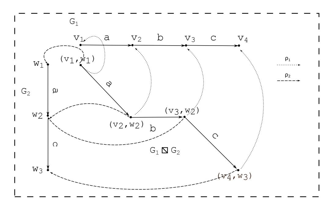
Figure 4. Weak-homomorphisms \(\rho_1\) from \(G_1 \boxtimes G_2\) to \(G_1\) and \(\rho_2\) from \(G_1 \boxtimes G_2\) to \(G_2\)

3. Basic Properties of the VRSP

We start with propositions on identity, the empty graph, commutativity and idem-potency, which are easy to prove. We use deterministic graphs, because of the required idem-potency of components. An example of a non-deterministic graph is given in Figure 5.

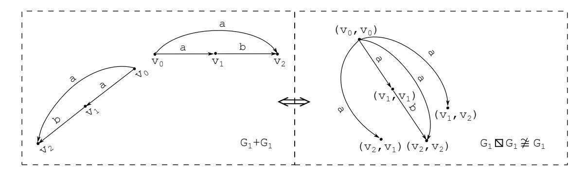
Figure 5. Non-deterministic and not idem-potent component.

We state the six propositions without proof.

Let G be a finite directed acyclic labelled multi-graph.

Proposition 3.1. \(G \boxtimes I \cong G\).

Proposition 3.2. G + G = G.

Proposition 3.3. \(G \boxtimes G_{\varnothing} = G_{\varnothing}\).

Let \(G_1\), \(G_2\) and \(G_3\) be deterministic finite directed acyclic labelled multi-graphs, in which all components are pairwise consistent in Proposition 3.4 through 3.6. Note that \(G_1\), \(G_2\) and \(G_3\) are pairwise vertex disjoint. This follows directly from \(G_1\), \(G_2\) and \(G_3\) being components.

Proposition 3.4. The synchronised product of \(G_1\) and \(G_2\) is commutative up to isomorphism. So \(G_1 \boxtimes G_2 \cong G_2 \boxtimes G_1\).

Proposition 3.5. The synchronised product of \(G_1\) and \(G_1\), \(G_1 \boxtimes G_1\) is idem-potent up to isomorphism. So \(G_1 \boxtimes G_1 \cong G_1\).

Note that an arc \(u_i v_i \in A(G_1)\) and an arc \(u_j v_j \in A(G_1)\), with \(\lambda(u_i v_i) = \lambda(u_j v_j)\), \(i \neq j\), \((u_i, u_j)\) has level > 0 in \(G_1 \square G_1\) and level = 0 in \(G_1 \square G_1\) (possibly after removing vertices with the same condition) and therefore \((u_i, u_j)\) (and consequently \((u_i, u_j)(v_i, v_j)\)) will be removed.

Proposition 3.6. The addition over \(G_1\) and \(G_1\), \(G_1 + G_1\) is idem-potent. So \(G_1 + G_1 = G_1\).

Propositions 3.1, 3.3, 3.4 and 3.5 follow directly from the definition of the synchronised product.

The synchronised product does not distribute over the addition up to isomorphism. So \(G_1 \boxtimes (G_2 + G_3) \ncong (G_1 \boxtimes G_2) + (G_1 \boxtimes G_3)\). This follows from the example shown in Figure 6. The set of label pairs used by VRSP are restricted to the label pairs in the components that are multiplied.

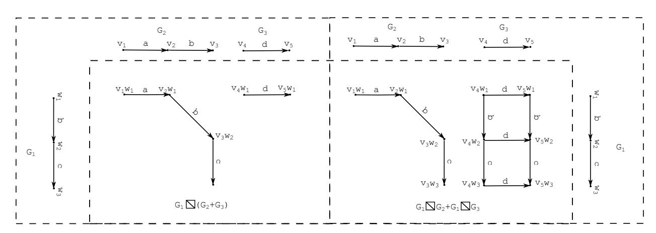
Figure 6. \(\square\) does not distribute over +.

The propositions 3.1 through 3.3 are necessary for Theorem 3.1.

Theorem 3.1. Let G be a finite deterministic directed acyclic labelled multi-graph, consisting of components \(G_1, G_2, G_3\), where \(G_1, G_2, G_3, G_1 \square G_2, G_1 \square G_3\) and \(G_2 \square G_3\) are pairwise consistent. Then the synchronised product is associative up to isomorphism. In particular, given components \(G_1, G_2\), and \(G_3\), the map \(\phi((u_1, u_2), u_3) = (u_1, (u_2, u_3))\) is an isomorphism from \((G_1 \square G_2) \square G_3\) to \(G_1 \square (G_2 \square G_3)\).

Proof. Assume there is a full path \(x_1 \ldots x_m\) in \(G_1 \boxtimes (G_2 \boxtimes G_3)\) and any full path \(t_1 \ldots t_o\) in \((G_1 \boxtimes G_2) \boxtimes G_3\), such that \(x_1 \ldots x_m \not\cong t_1 \ldots t_o\).

Because G¹ and G² n G³ are consistent, there exist weak-homomorphisms ρ¹ and ρ² with a full path u¹ . . . uⁱ in G1, where ρ1px¹ . . . xmq u¹ . . . uⁱ and a full path y¹ . . . y^l in G² n G3, where ρ2px¹ . . . xmq y¹ . . . y^l . Then there exist weak-homomorphisms ρ³ and ρ⁴ with a full path v¹ . . . v^j in G2, where ρ3py¹ . . . ylq v¹ . . . v^j and a full path w¹ . . . w^k in G3, where ρ4py¹ . . . ylq w¹ . . . wk. But, due to Corollary 2.2, because u¹ . . . uⁱ is a full path in G¹ and v¹ . . . v^j is a full path in G2, there is a full path z¹ . . . zⁿ in G¹ n G2. For these two full paths w¹ . . . z^k and z¹ . . . zⁿ there is a full path t¹ . . . t^o in pG¹ n G2q n G3, contradicting our assumption.

Thus for every full path in G1npG2nG3q there exists a full path in pG1nG2qnG3. Analogously for every full path in pG¹ n G2q n G³ there exists a full path in G¹ n pG² n G3q.

Therefore \[G_1 \boxtimes (G_2 \boxtimes G_3) \cong (G_1 \boxtimes G_2) \boxtimes G_3\].

Figure 7 shows the weak-homomorphisms ρⁱ from a set of full paths of the VRSP of two components to these components. Associativity is necessary to calculate the number of possible leaf covers of a target tree D by the Bell number, given in Section 4.

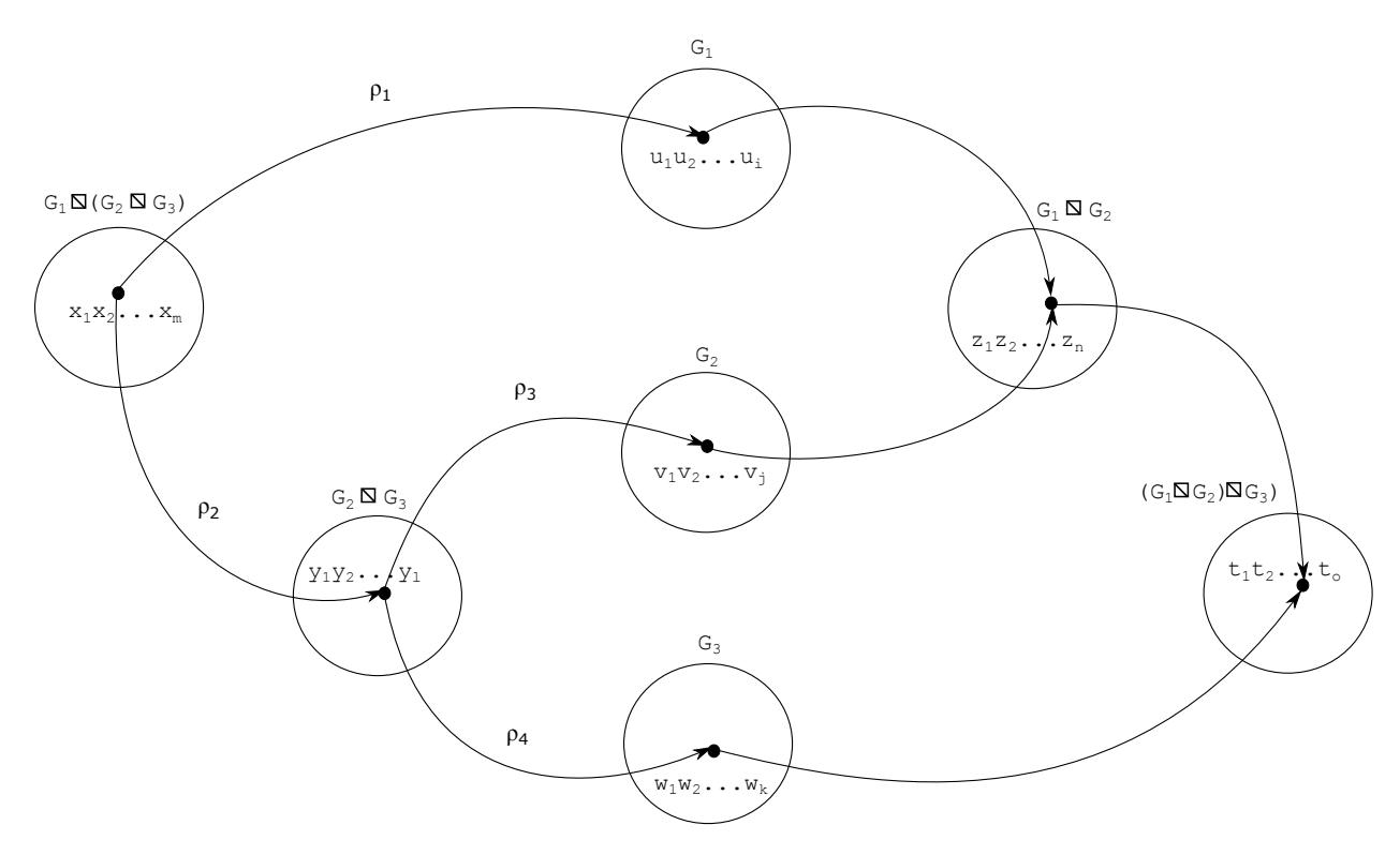
Figure 7. Weak-homomorphisms from sets of full paths to sets of full paths.

4. Feasibility of a Target Tree

Let D be a target tree. Recall that the leaves of D represent processes as specified by the designer of the periodic real-time application. A leaf cover of D is a solution if it represents a set of (combined) processes that meet their deadlines and fit in the available memory. The

cardinality of the set of leaf covers of all target trees over n leaves is given by the Bell number ,

\[B_n = \sum_{k=0}^{n-1} {n-1 \choose k} B_k, B_0 = 1, [1].\]

Because for two isomorphic target trees the order in which VRSP is executed over components can be different, the synchronised product of the components of the graph G has to be associative (G¹ n pG² n G3q pG¹ n G2q n G3) and commutative (G¹ n G² G² n G1). For this reason the components in the graph G have to be consistent. Moreover each product of components has to be consistent with the other remaining components.

Figure 8 gives an example where G1, G² and G³ are pairwise consistent. But G¹ n G² and G³ are not pairwise consistent.

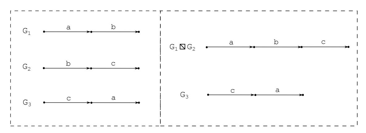
Figure 8. VRSP does not preserve consistency.

Therefore a heuristic has to check whether the components are still consistent after every multiplication by VRSP.

5. Synchronised Product Decision Problem

The cardinality of the set of leaf covers of all target trees over n leaves has an exponential distribution. We show that a leaf cover of a target tree D can be checked in polynomial time.

Definition 1. A monoid pG, n q is an algebraic structure which is closed under the associative operator n and has the identity element I, where G is generated by G under n.

Definition 2. Synchronised Product Decision Problem (SPDP) Let pG, n q be a monoid, together with a memory budget M and a deadline D. Can a feasible target tree D on V pGq be constructed?

Note that G ° n is represented by a leaf cover of D.

SPDP is in NP if there exists some oracle that points out a solution and there exists an algorithm that can check the solution in polynomial time. To formalise this, we need the following definitions, let:

• Aipaq be the set of arcs taⁱ |aⁱ P Aⁱ ^ λpaiq au

On a directed tree problem motivated by a newly introduced graph product | Antoon H. Boode et al.

• \(\mathcal{A}_k^{ij}(a)\) be the arc-set \(A_k(a)\) where k=i if \(|A_i(a)| \leq |A_j(a)|\) else k=j
• \(H_{ij}\) be the graph with arc-set \(A = \sum_{a} A_k^{ij}(a)\) and vertex-set \(\{v | v \in V \land A = V \times V\}\).

Then \[|A_1| + \cdots + |A_n| \le |A_{1 \boxtimes \cdots \boxtimes n}| + |\sum_{i=1}^{n-1} \sum_{j=i+1}^n A(H_{ij})|\].

\(m(\sum_{i=1}^{n-1}\sum_{j=i+1}^{n}H_{ij})\) can be calculated in polynomial time. For all \(i,j,i\neq j,\) \(m(G_i)+m(G_j)\geqslant\)

\[m(H_{ij})\]. So \(m(G_i) + m(G_j) - m(H_{ij}) \le m(G_i \square G_j)\). As soon as \(m(G_{\square}^{\Sigma}) - \sum_{i=1}^{n-1} \sum_{j=i+1}^{n} m(H_{i,j}) > \mathcal{M}\)

the calculation can stop, as further multiplications will not lead to a solution. In this case, \(G^{\Sigma}_{\square}\) is not a solution that full-fills the requirements for the deadline and memory occupancy.

Remark 5.1. This is only true because the components (and the products of the components) are consistent. Furthermore, the calculation is not performed in the target system but in a general purpose computing system, so the available memory may be significantly greater than the memory available in the target system.

Having calculated the synchronised product \(G^\Sigma_{\square}\) and performing a breadth first search for each component, we obtain the length of \(G^\Sigma_{\square}\), \(\ell(G^\Sigma_{\square})\). Therefore we have in polynomial time an answer whether the oracle's solution is valid. Because \(G^\Sigma_{\square}\) is represented by a leaf cover in the target tree D, a valid solution implies that D is feasible.

For these reasons SPDP is in NP.

Leung [7] defines the 0/1-Knapsack Decision Problem (KDP). Given a set \(U = \{u_1, u_2, \cdots, u_n\}\) with each item \(u_j\) having a size \(s_j\) and a value \(v_j\), a knapsack with size K, and a bound B. Is there a subset \(U' \subseteq U\) such that \(\sum_{u_j \in U'} s_j \leqslant K\) and \(\sum_{u_j \in U'} v_j \geqslant B\).

Theorem 5.1. SPDP is NP-complete.

Proof. Let \(G = \sum_{i=1}^{n} G_i\), \(\ell(G) = \sum_{i=1}^{n} \ell(G_i) = \mathcal{T}\). Let \(v_j\) be a vertex in a leaf cover LC with cardinality k of D, where D is a target tree generated by G.

Suppose \(U=\{u_1,\cdots,u_k\}\) is a solution for the 0/1 Knapsack Decision Problem, with \(u_j\) having size \(s_j=m(v_j)=\frac{\mathcal{M}}{m_j}, \sum\limits_{j=1}^k\frac{1}{m_j}\leqslant 1\) and value \(u_j'=\frac{\mathcal{T}}{k_j}-\ell(v_j), \sum\limits_{j=1}^k\frac{1}{k_j}\leqslant 1, K=\mathcal{M},\) \(B=\mathcal{T}-\mathcal{D}.\)

\(B = \mathcal{T} - \mathcal{D}.\)Because \(\sum_{i=1}^k s_i = \sum_{j=1}^k m(v_j) \leqslant \mathcal{M} = K\) and \(\sum_{j=1}^k \ell(v_j) \leqslant \mathcal{D} \Rightarrow \ell(G) - \ell(LC) \geqslant \mathcal{T} - \mathcal{D} = B\), LC is a solution for SPDP.

Conversely, if LC is a solution for SPDP, then \(\ell(LC) \leqslant \mathcal{D}\) and \(m(LC) \leqslant \mathcal{M} = K\), therefore \(\sum_{j=1}^k s_j \leqslant \mathcal{M} = K\) and \(\ell(LC) \leqslant \mathcal{D} \Rightarrow \sum_{i=1}^k u_i' = \mathcal{T} - \sum_{i=1}^k \ell(v_i) \geqslant \mathcal{T} - \mathcal{D} = B\). So U is a solution for the 0/1 Knapsack Problem.

This means that, for a Yes-instance of the 0/1 Knapsack Decision Problem, the constructed instance of the decision version of SPDP is a Yes-instance and, conversely, for a Yes-instance of the SPDP, the constructed instance of the decision version of 0/1 Knapsack Decision Problem is a Yes-instance. As the 0/1 Knapsack Decision Problem is NP-complete and SPDP is in NP, SPDP is NP-complete.

6. Heuristics

In [3] we describe three heuristics that give an answer for SPDP in polynomial time. The heuristics multiply using VRSP for a graph G °n i1 Gⁱ up to k ¤ n components. These heuristics are based on the (number of) actions that synchronise. All heuristics choose two components out of a series of n components, where

• the Largest Alphabetical Intersection (LAI) heuristic calculates the cardinality of the largest intersection of the alphabets of two components,
• the Maximising Synchronising Arcs (MSA) heuristic calculates the largest number of synchronising arcs of two components,
• the Minimising Not Synchronising Arcs (MNSA) heuristic calculates the smallest cardinality of the not-synchronising arcs set of two components.

Another approach is taking the VRSP of components Gⁱ and G^j (containing synchronising arcs) where the two components chosen for multiplication have the smallest occupancy of memory. This gives the Minimising Memory Occupancy (MMO) heuristic. So for Gⁱ , G^j , mpGⁱ n G^j q pmpGiq mpG^j qq is the minimum of all VRSPs mpG^k n Glq pmpGkq mpGlqq (containing synchronising arcs) taken over G1, Gn.

Let LC be a leaf cover of the target tree D with cardinality 1. Then,

• 1. if mpLCq ¤ M and `pLCq ¤ D, LC is a solution for the optimisation problem of G.
• 2. if mpLCq ¤ M and `pLCq ¡ D, there exists no solution for the optimisation problem of G,
• 3. if mpLCq ¡ M and `pLCq ¤ D, a solution may exist for the optimisation problem of G,
• 4. if mpLCq ¡ M and `pLCq ¡ D, there exists no solution for the optimisation problem of G.

Remark 6.1. The solution may not be optimal. That depends on the requirements with respect to memory occupancy and processor utilisation.

As the same reasoning as for "SPDP is in NP" is valid, if mpLCq ¤ M then items 1 and 2 can be calculated in polynomial time. For item 4 no solution exists, because `pLCq ¡ D [4]. This can be calculated in polynomial time, because as soon as for a leaf cover LC¹ , mpLC¹ q ¡ M n°1 °n mpHij qq the algorithm can stop as no solution exists.

i1 ji1 Remains item 3, where mpLCq ¡ M and `pLCq ¤ D. As SPDP is NP-complete, an optimal solution cannot be found in polynomial time (unless P=NP). We compare the three algorithms in

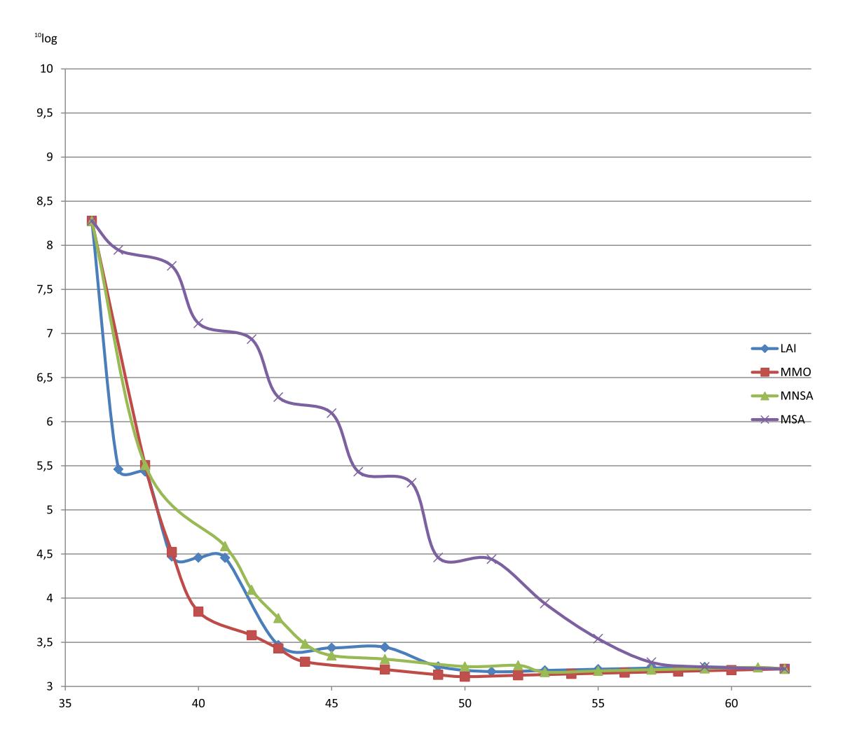
Figure 9. Deadlines and Memory Occupancy of MNSA, LAI, MMO and MSA.

[3] together with the algorithm introduced in this paper, Minimal Memory Occupancy (MMO), given in the Appendix, Algorithm 2.

The level of the tail of a synchronising arc determines whether LAI or MMO will perform better. For two components where these levels are low in one component and high in the other component, MMO will perform better because the VRSP over these two components will be (almost) optimal with respect to memory occupancy. Whereas LAI may choose two components with a larger alphabetical intersection that have the levels for tails of the synchronising arcs that are relatively on the same level. But with respect to the length of the product of the components this can be the opposite.

In Figure 9 we give for the Production Cell case study in [3] the results for the four algorithms, MNSA, LAI, MSA and MMO. Note the logarithmic scale in the y-abyss. Due to the specification of the processes where each process synchronises over at least one action with all other processes, MMO performs best up till the last multiplication. To achieve a length of 37 LAI has the best (is minimal) memory occupancy.

The algorithms replace two components by their product until all components are multiplied. So from a leaf cover with cardinality n to a leaf cover with cardinality 1.

7. Conclusions

A set of processes that does not meet its deadline or does not fit in the available memory can, under certain conditions, be transformed into a set of processes that will fulfil both requirements. For this transformation we use our Vertex Removing Synchronised Product (VRSP) on consistent finite labelled weighted deterministic directed acyclic multi-components.

We have given a definition for consistency such that consistent components are deadlock free. This is essential for the processes represented by these components, because otherwise in the target system deadlines will be missed. Missing a deadline leads to a catastrophe in hard realtime systems.

We have given conditions and proof for VRSP to be commutative, associative and idem-potent. This is necessary because otherwise components may not be pairwise consistent.

We have introduced a directed tree problem motivated by VRSP in the context of periodic hard real-time processes. The number of target trees is exponential with respect to the number of components, representing the original set of processes and is given by the Bell number. We have dealt with the graph theoretical and computational complexity issues. We have shown that the directed tree problem is NP-complete and we have presented and compared several heuristics for this problem.

Because SPDP is NP-complete, in practice heuristics have to be used (like MMO and the ones we proposed in [3]) to calculate a set of components which represent processes that will not be tardy and fit in the available memory. We have introduced a new heuristic based on memory occupancy that shows for our case study that its performance is in most cases better than the heuristics given in [3].

In our case the new set of processes is calculated off-line during the design process and forms no burden on the target system, in our case an active real-time system.

Because the components have to be consistent, to compose the original set of components, the designer is limited in his description of the system. In our view this is not a problem, because, if the set of graphs would be not consistent, it contains graphs that represent processes that form a deadlock. This is a situation that has to be avoided.

Acknowledgement

The authors would like to express their gratitude to the anonymous reviewers for their useful suggestions and comments. The research of the first author has been funded by the InHolland University of Applied Sciences, Alkmaar, The Netherlands.

References

• [1] E. T. Bell, Exponential polynomials. Annals of Mathematics, 35(2) (1934), 258–277.
• [2] J.A. Bondy and U.S.R. Murty, Graph Theory, Springer, Berlin, 2008.

• [3] A. H. Boode and J. F. Broenink, Performance of periodic real-time processes: a vertexremoving synchronised graph product, Communicating Process Architectures 2014, 36th WoTUG conference on concurrent and parallel programming, Bicester, Open Channel Publishing Ltd. (2014), 119–138.
• [4] A. H. Boode, H. J. Broersma, and J. F. Broenink, Improving the performance of periodic realtime processes: a graph theoretical approach, Communicating Process Architectures 2013, 35th WoTUG conference on concurrent and parallel programming, Bicester, Open Channel Publishing Ltd. (2013), 57–79.
• [5] Richard Hammack, Wilfried Imrich, and Sandi Klavzar, ˇ Handbook of product graphs, Discrete Mathematics and its Applications (Boca Raton). CRC Press, Boca Raton, FL, second edition, 2011.
• [6] P. Hell and J. Neset ˇ ˇril, Graphs and Homomorphisms, Oxford Lecture Series in Mathematics and Its Applications. OUP Oxford, 2004.
• [7] Joseph YT Leung, Handbook of scheduling: algorithms, models, and performance analysis, CRC Press, 2004.
• [8] Jeff Magee and Jeff Kramer, Concurrency: State Models &Amp; Java Programs, John Wiley & Sons, Inc., New York, NY, USA, 1999.
• [9] R. Milner, Communication and Concurrency, Prentice-Hall, Inc., Upper Saddle River, NJ, USA, 1989.
• [10] Stefan Wohrle and Wolfgang Thomas, Model checking synchronized products of infinite ¨ transition systems, Proc. 19th LICS, IEEE Comp. Soc (2004), 2–11.

Appendix

The Largest Alphabetical Intersection (LAI) heuristic is an exact copy of the LAI algorithm given in [3]. MMO is almost identical to LAI, but requires more computation, as the VRSP of all products has to be calculated. Both are very simple straightforward algorithms, that fit in the algorithms given in [3]. No attempt has been made to optimise these algorithms, although that is necessary for usage in a tool-chain.

Algorithm 1 Calculating the Largest Alphabetical Intersection

 \begin{array}{lll} \operatorname{Require:} & G = \sum\limits_{i=1}^k G_i \\ 1: & first & = 1 \\ 2: & second = 2 \\ 3: & num & = 0 \\ 4: & for i = 1 \text{ to } k - 1 \text{ do} \\ 5: & for j = i + 1 \text{ to } k \text{ do} \\ 6: & newNum = |L(G_i) \cap L(G_j)| \\ 7: & \text{ if } (newNum > num) \text{ then} \\ 8: & num & \leftarrow newNum \\ 6: & first & \leftarrow i \\ 10: & second \leftarrow j \\ 11: & \operatorname{return} \ (first, second) \\ \end{array}

Algorithm 2 Calculating the Minimal Memory Occupancy

Require: G = \sum\limits_{i=1}^k G_i

1: first = 1
2: second = 2
3: mem = \infty
4: for i = 1 to k - 1 do
5: for j = i + 1 to k do
6: newMEM = m(G_i \square G_j)
7: if (newMEM < mem) then
8: num \leftarrow newNum
9: first \leftarrow i
10: second \leftarrow j
11: return \ (first, second)