Cristina Dalfo, Miquel ´ Angel Fiol ` ^a , Margarida Mitjana^b

^aDepartament de Matematica Aplicada IV, ` Universitat Politecnica de Catalunya, ` Barcelona, Catalonia ^bDepartament de Matematica Aplicada I, ` Universitat Politecnica de Catalunya, ` Barcelona, Catalonia

cdalfo@ma4.upc.edu, fiol@ma4.upc.edu, margarida.mitjana@upc.edu

We study a family of graphs related to the n-cube. The middle cube graph of parameter k is the subgraph of Q2k−¹ induced by the set of vertices whose binary representation has either k − 1 or k number of ones. The middle cube graphs can be obtained from the well-known odd graphs by doubling their vertex set. Here we study some of the properties of the middle cube graphs in the light of the theory of distance-regular graphs. In particular, we completely determine their spectra (eigenvalues and their multiplicities, and associated eigenvectors).

Keywords: distance-regular graph, odd graph, spectrum Mathematics Subject Classification : 05C50

DOI: 10.5614/ejgta.2015.3.2.3

1. Introduction

The n-cube Qn, or n-dimensional hypercube, has been extensively studied. Nevertheless, many open questions remain. Harary, Hayes, and Wu wrote a comprehensive survey on hypercube graphs [20]. Recall that the n-cube Qⁿ has vertex set V = {0, 1} n , and n-tuples representing vertices are adjacent if and only if they differ in exactly one coordinate. Then, Qⁿ is an n-regular

Received: 11 January 2015, Revised: 23 May 2015, Accepted: 27 May 2015.

bipartite graph with \(2^n\) vertices. It is natural to consider its vertex set as partitioned into n+1 layers, the layer \(L_k\) consisting of the \(\binom{n}{k}\) vertices containing exactly k 1s, for \(0 \le k \le n\). Seeing the vertices of \(Q_n\) as the characteristic vector of subsets of \([n] = \{1, 2, \ldots, n\}\), the vertices of layer \(L_k\) correspond to the subsets of cardinality k, while the adjacencies correspond to the inclusion relation.

If n is odd, n=2k-1, the middle two layers \(L_k\) and \(L_{k-1}\) of \(Q_n\) have the same number \(\binom{n}{k}=\binom{n}{k-1}\) of vertices. Then the middle cube graph, denoted by \(MQ_k\), is the graph induced by these two layers. It has been conjectured by Dejter, Erdős, and Havel [21] among others, that \(MQ_k\) is Hamiltonian. It is known that the conjecture holds for \(n \leq 16\) (see Savage and Shields [26]), and it was almost solved by Robert Johnson [25].

In this paper we study some of the properties of the middle cube graphs in the light of the theory of distance-regular graphs. In particular, we completely determine their spectra (eigenvalues and their multiplicities, and associated eigenvectors). In this context, Qiu and Das provided experimental results for eigenvalues of several interconnection networks for which no complete characterization were known (see [24, §3.2]).

Before proceeding with our study, we fix some basic definitions and notation used throughout the paper. We denote by G = (V, E) a (simple, connected and finite) graph with vertex set V an edge set E. The order of the graph G is n = |V| and its size is m = |E|. We label the vertices with the integers \(1, 2, \dots, n\). If i is adjacent to j, that is, \(ij \in E\), we write \(i \sim j\) or \(i \stackrel{(E)}{\sim} j\). The distance between two vertices is denoted by \(\operatorname{dist}(i,j)\). We also use the concepts of even distance and odd distance between vertices (see Bond and Delorme [6]), denoted by dist⁺ and dist^-, respectively. They are defined as the length of a shortest even (respectively, odd) walk between the corresponding vertices. The set of vertices which are \(\ell\)-apart from vertex i, with respect to the usual distance, is \(\Gamma_{\ell}(i) = \{j : \operatorname{dist}(i,j) = \ell\}\), so that the degree of vertex i is simply \(\delta_i := |\Gamma_1(i)| \equiv |\Gamma(i)|\). The eccentricity of a vertex is \(ecc(i) := \max_{1 \le i \le n} dist(i, j)\) and the diameter of the graph is \(D \equiv D(G) := \max_{1 \le i \le n} \operatorname{ecc}(i)\). Given \(0 \le \ell \le D\), the distance-\(\ell\)graph \(G_{\ell}\) has the same vertex set as G and two vertices are adjacent in \(G_{\ell}\) if and only if they are at distance \(\ell\) in G. An antipodal graph G is a connected graph of diameter D for which \(G_D\) is a disjoint union of cliques. In this case, the folded graph of G is the graph \(\overline{G}\) whose vertices are the maximal cliques of \(G_D\) and two vertices are adjacent if their union contains an edge of G. If, moreover, all maximal cliques of \(G_D\) have the same size r, then G is also called an antipodal r-cover of \(\overline{G}\) (double cover if r=2, triple cover if r=3, etc.).

Recall that a graph G with diameter D is distance-regular when, for all integers \(h, i, j \ (0 \le h, i, j \le D)\) and vertices \(u, v \in V\) with \(\operatorname{dist}(u, v) = h\), the numbers

\[p_{ij}^h = |\{w \in V : \operatorname{dist}(u,w) = i, \operatorname{dist}(w,v) = j\}|\]

do not depend on u and v. In this case, such numbers are called the intersection parameters and, for notational convenience, we write \(c_i = p_{1i-1}^i\), \(b_i = p_{1i+1}^i\), and \(a_i = p_{1i}^i\) (see Brouwer, Cohen, and Neumaier [7] and Fiol [11]).

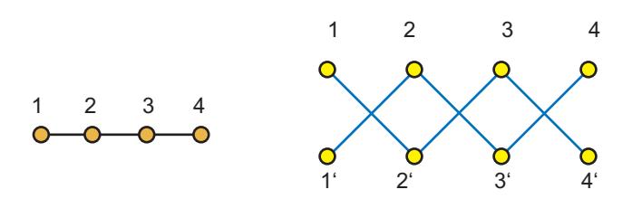
Figure 1. The path \(P_4\) and its bipartite double graph.

2. Preliminaries

2.1. The odd graphs

The odd graph, independently introduced by Balaban, Farcussiu, and Banica [2] and Biggs [3], is a family of graphs that has been studied by many authors (see Biggs [4, 5] and Godsil [18]). More recently, Fiol, Garriga, and Yebra [16] introduced the twisted odd graphs, which share some interesting properties with the odd graphs although they have, in general, a more involved structure.

For \(k \geq 2\), the odd graph \(O_k\) has vertices representing the (k-1)-subsets of \([2k-1] = \{1, 2, \ldots, 2k-1\}\), and two vertices are adjacent if and only if they are disjoint. For example, \(O_2\) is the complete graph \(K_3\), and \(K_3\) is the Petersen graph. In general, \(K_3\) is a \(K_4\)-regular graph on \(K_3\) vertices, diameter \(K_3\) and \(K_4\) if \(K_4\) and \(K_4\) if \(K_4\) (see Biggs [5]).

The odd graph \(O_k\) is a distance-regular graph with intersection parameters

\[b_j = k - \left[ \frac{j+1}{2} \right], \quad c_j = \left[ \frac{j+1}{2} \right] \quad 0 \le j \le k-1.\]

With respect to the spectrum, the distinct eigenvalues of \(O_k\) are \(\lambda_i = (-1)^i (k-i)\), \(0 \le i \le k-1\), with multiplicities

\[m(\lambda_i) = {2k-1 \choose i} - {2k-1 \choose i-1} = \frac{k-i}{k} {2k \choose i}.\]

2.2. The bipartite double graph

Let G = (V, E) be a graph of order n, with vertex set \(V = \{1, 2, ..., n\}\). Its bipartite double graph \(\widetilde{G} = (\widetilde{V}, \widetilde{E})\) is the graph with the duplicated vertex set \(\widetilde{V} = \{1, 2, ..., n, 1', 2', ..., n'\}\), and adjacencies induced from the adjacencies in G as follows:

\[i \stackrel{(E)}{\sim} j \Rightarrow \begin{cases} i \stackrel{(\tilde{E})}{\sim} j', \text{ and} \\ j \stackrel{(\tilde{E})}{\sim} i'. \end{cases}\] (1)

Thus, the edge set of \(\widetilde{G}\) is \(\widetilde{E} = \{ij' | ij \in E\}\).

From the definition, it follows that \(\widetilde{G}\) is a bipartite graph with stable subsets \(V_1 = \{1, 2, \dots, n\}\) and \(V_2 = \{1', 2', \dots, n'\}\). For example, if G is a bipartite graph, then its bipartite double graph \(\widetilde{G}\) consists of two non-connected copies of G (see Figure 1).

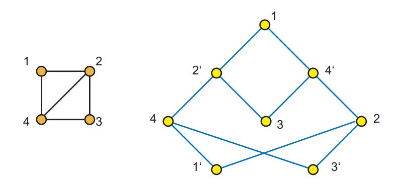
Figure 2. Graph G has diameter 2 and \(\widetilde{G}\) has diameter 3.

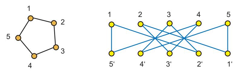
Figure 3. \(C_5\) and its bipartite double graph.

The bipartite double graph \(\widetilde{G}\) has an involutive automorphism without fixed edges, which interchanges vertices i and i'. On the other hand, the map from \(\widetilde{G}\) onto G defined by \(i' \mapsto i\), \(i \mapsto i\) is a 2-fold covering.

If G is a \(\delta\)-regular graph, then \(\widetilde{G}\) also is. Moreover, if the degree sequence of the original graph G is \(\delta = (\delta_1, \delta_2, \dots, \delta_n)\), the degree sequence for its bipartite double graph is \(\widetilde{\delta} = (\delta_1, \delta_2, \dots, \delta_n, \delta_1, \delta_2, \dots, \delta_n)\).

The distance between vertices in the bipartite double graph \(\widetilde{G}\) can be given in terms of the even and odd distances in G. Namely,

\[\operatorname{dist}_{\widetilde{G}}(i,j) = \operatorname{dist}_{G}^{+}(i,j)\]
\[\operatorname{dist}_{\widetilde{G}}(i,j') = \operatorname{dist}_{G}^{-}(i,j).\]

Note that always \(\mathrm{dist}_G^-(i,j)>0\) even if i=j. Actually, \(\widetilde{G}\) is connected if and only if G is connected and non-bipartite.

More precisely, it was proved by Bond and Delorme [6] that if G is a non-bipartite graph with diameter D, then its bipartite double graph \(\widetilde{G}\) has diameter \(\widetilde{D} \leq 2D+1\), and \(\widetilde{D}=2D+1\) if and only if for some vertex \(i \in V\) the subgraph induced by the vertices at distance less than D from i, \(G_{\leq D-1}(i)\), is bipartite.

In Figures 2-5, we can see the bipartite double graph of three different graphs. The cycle \(C_5\) and Petersen graph both have diameter D=2, and their bipartite double graphs have diameter \(\widetilde{D}=2D+1=5\), while in the first example (Figure 2) \(\widetilde{G}\) has diameter \(\widetilde{D}=3<2D+1\).

The extended bipartite double graph \(\widehat{G}\) of a graph G is obtained from its bipartite double graph by adding edges (i, i') for each \(i \in V\). Note that when G is bipartite, then \(\widehat{G}\) is the direct product \(G \square K_2\).

Figure 4. \(C_5\) and \(C_{10}\) as another view of its bipartite double graph.

Figure 5. Petersen's graph and its bipartite double graph.

2.3. Spectral properties of the bipartite double graph

Let us now recall a useful result from spectral graph theory. For any graph, it is known that the components of its eigenvalues can be seen as charges on each vertex (see Fiol and Mitjana [17] and Godsil [19]). Let G = (V, E) be a graph with adjacency matrix \(\boldsymbol{A}\) and \(\lambda\)-eigenvector \(\boldsymbol{v}\). Then, the charge of vertex \(i \in V\) is the entry \(v_i\) of \(\boldsymbol{v}\), and the equation \(\boldsymbol{A}\boldsymbol{v} = \lambda \boldsymbol{v}\) means that the sum of the charges of the neighbors of vertex i is \(\lambda\) times the charge of vertex i:

\[(\boldsymbol{A}\boldsymbol{v})_i = \sum_{i \stackrel{(E)}{\sim} j} v_j = \lambda v_i.\]

In what follows we compute the eigenvalues of the bipartite double graph \(\widetilde{G}\) and the extended bipartite double graph \(\widehat{G}\) as functions of the eigenvalues of a non-bipartite graph G. We also show how to obtain the eigenvalues together with the corresponding eigenvectors of \(\widetilde{G}\) and \(\widehat{G}\).

First, we recall the following technical result, due to Silvester [27], on the determinant of some block matrices:

Theorem 2.1. Let F be a field and let R be a commutative subring of F n×n , the set of all n × n matrices over F. Let M ∈ R^m×^m, then

\[det_F(\mathbf{M}) = det_F(det_R(\mathbf{M})).\]

For example, if M = A B C D , where A, B, C, D are n×n matrices over F which commute with each other, then Theorem 2.1 reads

\[det_F(\mathbf{M}) = det_F(\mathbf{AD} - \mathbf{BC}). \tag{2}\]

Now we can use the above theorem to find the characteristic polynomial of the bipartite double and the extended bipartite double graphs.

Theorem 2.2. Let G be a graph on n vertices, with the adjacency matrix A and characteristic polynomial ^φG(x). Then, the characteristic polynomials of ^Ge and ^Gb are, respectively,

\[\phi_{\widetilde{G}}(x) = (-1)^n \phi_G(x) \phi_G(-x), \tag{3}\]

\[\phi_{\widehat{G}}(x) = (-1)^n \phi_G(x-1) \phi_G(-x-1).\] (4)

Proof. From the definitions of ^Ge and ^Gb, their adjacency matrices are, respectively,

\[\widetilde{A} = \begin{pmatrix} O & A \ A & O \end{pmatrix} \ \ \text{and} \ \ \widehat{A} = \begin{pmatrix} O & A+I \ A+I & O \end{pmatrix}.\]

Thus, by (2), the characteristic polynomial of ^Ge is

\[\phi_{\widetilde{G}}(x) = \det(x\boldsymbol{I}_{2n} - \widetilde{\boldsymbol{A}}) = \det\begin{pmatrix} x\boldsymbol{I}_n & -\boldsymbol{A} \\ -\boldsymbol{A} & x\boldsymbol{I}_n \end{pmatrix} = \det(x^2\boldsymbol{I}_n - \boldsymbol{A}^2)\]\[= \det(x\boldsymbol{I}_n - \boldsymbol{A})\det(x\boldsymbol{I}_n + \boldsymbol{A}) = (-1)^n\phi_G(x)\phi_G(-x),\]

whereas, the characteristic polynomial of ^Gb is

\[\phi_{\widehat{G}}(x) = \det(x\mathbf{I}_{2n} - \widehat{\mathbf{A}}) = \det\begin{pmatrix} x\mathbf{I}_n & -\mathbf{A} - \mathbf{I}_n \\ -\mathbf{A} - \mathbf{I}_n & x\mathbf{I}_n \end{pmatrix}\] \[= \det(x^2\mathbf{I}_n - (\mathbf{A} + \mathbf{I}_n)^2) = \det(x\mathbf{I}_n - (\mathbf{A} + \mathbf{I}_n)) \det(x\mathbf{I}_n + (\mathbf{A} + \mathbf{I}_n))\] \[= \det((x-1)\mathbf{I}_n - \mathbf{A})(-1)^n \det(-(x+1)\mathbf{I}_n - \mathbf{A})\] \[= (-1)^n \phi_G(x-1)\phi_G(-x-1).\]

As a consequence, we have the following corollary:

Corollary 2.1. Given a graph G with spectrum

\[\operatorname{sp} G = \{\lambda_0^{m_0}, \lambda_1^{m_1}, \dots, \lambda_d^{m_d}\},\\]

where the superscripts denote multiplicities, then the spectra of \(\widehat{G}\) and \(\widehat{G}\) are, respectively,

\[\operatorname{sp} \widetilde{G} = \{ \pm \lambda_0^{m_0}, \pm \lambda_1^{m_1}, \dots, \pm \lambda_d^{m_d} \},\] \[\operatorname{sp} \widehat{G} = \{ \pm (1 + \lambda_0)^{m_0}, \pm (1 + \lambda_1)^{m_1}, \dots, \pm (1 + \lambda_d)^{m_d} \}.\]

Proof. Just note that, by (3) and (4), for each root \(\lambda\) of \(\phi_G(x)\), \(\mu = \pm \lambda\) are roots of \(\phi_{\widetilde{G}}(x)\), whereas \(\mu = \pm (1 + \lambda)\) are roots of \(\phi_{\widehat{G}}(x)\).

Note that the spectra of \(\widetilde{G}\) and \(\widehat{G}\) are symmetric, as expected, because both \(\widetilde{G}\) and \(\widehat{G}\) are bipartite graphs.

In the next theorem we are concerned with the eigenvectors of \(\widehat{G}\) and \(\widehat{G}\), in terms of the eigenvectors of G. The computations also give an alternative derivation of the above spectra.

Theorem 2.3. Let G be a graph and \(\mathbf{v}\) a \(\lambda\)-eigenvector of G. Let us consider the vector \(\mathbf{u}^+\) with components \(u_i^+ = u_{i'}^+ = v_i\), and \(\mathbf{u}^-\), with components \(u_i^- = v_i\) and \(u_{i'}^- = -v_i\), for \(1 \le i, i' \le n\). Then,

• \(u^+\) is a \(\lambda\)-eigenvector of \(\widetilde{G}\) and a \((1 + \lambda)\)-eigenvector of \(\widehat{G}\);
• \(u^-\) is a \((-\lambda)\)-eigenvector of \(\widetilde{G}\) and a \((-1-\lambda)\)-eigenvector of \(\widehat{G}\).

Proof. In order to show that \(u^+\) is a \(\lambda\)-eigenvector of \(\widetilde{G}\), we distinguish two cases:

• Given vertex i, for \(1 \leq i \leq n\), all its adjacent vertices are of type j', with \(i \stackrel{(E)}{\sim} j\). Then

\[(\boldsymbol{A}\boldsymbol{u}^{+})_{i} = \sum_{j'\stackrel{(\widetilde{E})}{i}} u_{j'}^{+} = \sum_{j\stackrel{(E)}{\sim} i} v_{j} = \lambda v_{i} = \lambda u_{i}^{+}.\]

• Given vertex i', for \(1 \le i \le n\), all its adjacent vertices are of type j, with \(i \stackrel{(E)}{\sim} j\). Then

\[(\boldsymbol{A}\boldsymbol{u}^{+})_{i'} = \sum_{j \stackrel{(\widetilde{E})}{\sim} i'} u_{j}^{+} = \sum_{j \stackrel{(E)}{\sim} i} v_{j} = \lambda v_{i} = \lambda u_{i}^{+}.\]

By a similar reasoning with \(u^-\), we obtain

\[(\boldsymbol{A}\boldsymbol{u}^{-})_{i} = \sum_{j'} u_{j'}^{-} = -\sum_{j \stackrel{(E)}{\sim} i} v_{j} = -\lambda u_{i}^{-} \text{ and } (\boldsymbol{A}\boldsymbol{u}^{-})_{i'} = \sum_{j \stackrel{(E)}{\sim} i'} u_{j}^{-} = \sum_{j \stackrel{(E)}{\sim} i} v_{j} = -\lambda u_{i'}^{-}.\]

Therefore, \(u^-\) is a \((-\lambda)\)-eigenvector of the bipartite double graph \(\widetilde{G}\).

In the same way, we can prove that \(u^+\) and \(u^-\) are eigenvectors of \(\widehat{G}\) with respective eigenvalues \(1 + \lambda\) and \(-1 - \lambda\).

Notice that, for every linearly independent eigenvectors \(v_1\) and \(v_2\) of G, we get the linearly independent eigenvectors \(u_1^\pm\) and \(u_2^\pm\) of \(\widetilde{G}\). As a consequence, the geometric multiplicity of eigenvalue \(\lambda\) of G coincides with the geometric multiplicities of the eigenvalues \(\lambda\) and \(-\lambda\) of \(\widetilde{G}\), and \(1 + \lambda\) and \(-1 - \lambda\) of \(\widehat{G}\).

3. The middle cube graphs

For \(k \ge 1\) and n = 2k - 1, the middle cube graph \(MQ_k\) is the subgraph of the n-cube \(Q_n\) induced by the vertices whose binary representations have either k - 1 or k number of 1s. Then, \(MQ_k\) has order \(2\binom{n}{k}\) and is k-regular, since a vertex with k - 1 1s has k zeroes, so it is adjacent to k vertices with k 1s, and similarly a vertex with k 1s has k adjacent vertices with k - 1 1s (see Figures 6 and 7).

The middle cube graph \(MQ_k\) is a bipartite graph with stable sets \(V_0\) and \(V_1\) constituted by the vertices whose corresponding binary string has, respectively, even or odd \(Hamming\ weight\), that is, number of 1s. The diameter of the middle cube graph \(MQ_k\) is D=2k-1.

3.1. \(MQ_k\) is the bipartite double graph of \(O_k\)

Notice that, if A and B are both subsets of [2k-1], \(A \subset B\) if and only if A and \(\overline{B}\) are disjoint. Moreover, if |B| = k, then \(|\overline{B}| = k-1\). This gives the following result.

Proposition 3.1. The middle cube graph \(MQ_k\) is isomorphic to \(\widetilde{O}_k\), the bipartite double graph of \(O_k\).

Proof. The mapping from \(\widetilde{O}_k\) to \(MQ_k\) defined by:

\[\begin{array}{cccc} f: & V[\widetilde{O}_k] & \to & V[MQ_k] \\ & \boldsymbol{u} & \mapsto & \boldsymbol{u} \\ & \boldsymbol{u}' & \mapsto & \overline{\boldsymbol{u}} \end{array}\]

is clearly bijective. Moreover, according to the definition of bipartite double graph in (1), if u and v' are two vertices of \(\widetilde{O}_k\), then

\[\boldsymbol{u} \sim \boldsymbol{v}' \Leftrightarrow \boldsymbol{u} \cap \boldsymbol{v} = \varnothing \Leftrightarrow \boldsymbol{u} \subset \overline{\boldsymbol{v}},\]

which is equivalent to say that if \(u \sim v'\) in \(\widetilde{O}_k\), then \(f(u) = u \sim \overline{v} = f(v')\) in \(MQ_k\).

For example, the middle cube graph \(MQ_2\) contains vertices with one or two 1s in their binary representation. The adjacencies give simply a 6-cycle (see Figure 6), which is isomorphic to \(\widetilde{O}_2\). As another example, \(MQ_3\) has 20 vertices because there are \(\binom{5}{2}=10\) vertices with two 1s, and \(\binom{5}{3}=10\) vertices with three 1s in their binary representation (see Figure 7). Compare the Figures 5 and 7 in order to realize the isomorphism between the definitions of \(MQ_3\) and \(\widetilde{O}_3\).

It is known that \(O_k\) is a bipartite 2-antipodal distance-regular graph. See Biggs [5] and Brouwer, Cohen, and Neumaier [7] for more details.

3.2. Spectral properties

The spectrum of the hypercube \(Q_{2k-1}\) contains all the eigenvalues (including multiplicities) of the middle cube \(MQ_k\):

\[\operatorname{sp} MQ_k \subseteq \operatorname{sp} Q_{2k-1}.\]

Figure 6. The middle cube graph \(MQ_2\) as a subgraph of \(Q_3\) or as the bipartite double graph of \(O_2 = K_3\).

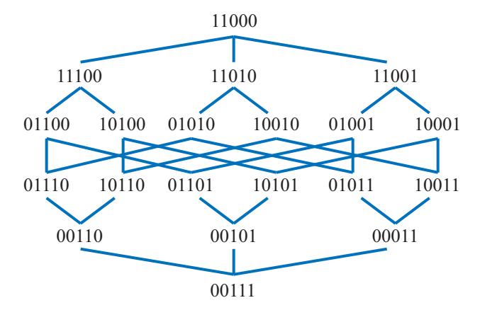
Figure 7. The middle cube graph \(MQ_3\).

According to the result of Corollary 2.1, the spectrum of the middle cube graph \(MQ_k\simeq \widetilde{O}_k\) can be obtained from the spectrum of the odd graph \(O_k\). The distinct eigenvalues of \(MQ_k\) are \(\theta_i^+=(-1)^i(k-i)\) and \(\theta_i^-=-\theta_i^+\), for \(0\leq i\leq k-1\), with multiplicities

\[m(\theta_i^+) = m(\theta_i^-) = \frac{k-i}{k} \binom{2k}{i}. \tag{5}\]

For example,

\[sp MQ_3 = \{\pm 2, \pm 1^2\}, sp MQ_5 = \{\pm 3, \pm 2^4, \pm 1^5\}, sp MQ_7 = \{\pm 4, \pm 3^6, \pm 2^{14}, \pm 1^{14}\}, sp MQ_9 = \{\pm 5, \pm 4^8, \pm 3^{27}, \pm 2^{48}, \pm 1^{42}\}.\]

The middle cube graph is a distance-regular graph. For instance, the distance polynomials of \(MQ_k\)

are

\[p_0(x) = 1,\] \[p_1(x) = x,\] \[p_2(x) = x^2 - 3,\] \[p_3(x) = \frac{1}{2}(x^3 - 5x),\] \[p_4(x) = \frac{1}{4}(x^4 - 9x^2 + 12),\] \[p_5(x) = \frac{1}{12}(x^5 - 11x^3 + 22x).\]

As the sum of the distance polynomials is the Hoffman polynomial [22], we have

\[\sum_{i=0}^{5} p_i(x) = \frac{1}{12}(x-1)(x-2)(x+3)(x+2)(x+1). \tag{6}\]

The eigenvalues of the \(MQ_3\) are \(\lambda_0 = 3\) and the zeroes of polynomial (6):

ev \[MQ_3 = \{3, 2, 1, -1, -2, -3\},\\]

and their multiplicities, \(m(\lambda_i)\), can be computed using the highest degree polynomial \(p_{2k-1}\), according to the result by Fiol [11]:

\[m(\lambda_i) = \frac{\phi_0 p_{2k-1}(\lambda_0)}{\phi_i p_{2k-1}(\lambda_i)}, \quad 0 \le i \le 2k-1,\]

where \(\phi_i = \prod_{j=0, j \neq i}^{2k-1} (\lambda_i - \lambda_j)\). Of course, this expression yields the same result as (5). Namely, \(m(\lambda_i) = m(\lambda_{2k-1-i}) = m(\theta_i^{\pm})\), for \(0 \le i \le k-1\).

The values of the highest degree polynomial are \(p_5(3) = p_5(1) = p_5(-1) = 1\) and \(p_5(2) = p_5(-1) = p_5(-3) = -1\). Moreover, \(\phi_0 = -\phi_5 = 240\), \(\phi_1 = -\phi_4 = -60\), and \(\phi_2 = -\phi_3 = 48\). Then,

\[m(\lambda_0) = m(\lambda_5) = m(\theta_0^{\pm}) = 1,\]
\(m(\lambda_1) = m(\lambda_4) = m(\theta_1^{\pm}) = 4,\)
\(m(\lambda_2) = m(\lambda_3) = m(\theta_2^{\pm}) = 5.\)

3.3. Middle cube graphs as boundary graphs

Let G be a graph with diameter D and distinct eigenvalues ev \(G = \{\lambda_0, \lambda_1, \dots, \lambda_d\}\), where \(\lambda_0 > \lambda_1 > \dots > \lambda_d\). A classical result states that \(D \leq d\) (see, for instance, Biggs [5]). Other results related to the diameter D and some (or all) different eigenvalues have been given by Alon and Milman [1], Chung [8], van Dam and Haemers [9], Delorme and Solé [10], and Mohar [23], among others. Fiol, Garriga, and Yebra [12, 14, 15] showed that many of these results can be stated with the following common framework: If the value of a certain polynomial P at \(\lambda_0\) is large enough, then the diameter is at most the degree of P. More precisely, it was shown that optimal

results arise when P is the so-called k-alternating polynomial, which in the case of degree d-1 is characterized by \(P(\lambda_i)=(-1)^{i+1}\) for \(1\leq i\leq d\), and satisfies \(P(\lambda_0)=\sum_{i=1}^d\frac{\pi_0}{\pi_i}\), where \(\pi_i=\prod_{j=0,j\neq i}^d|\lambda_i-\lambda_j|\). In particular, when G is a regular graph on n vertices, the following implication holds:

\[P(\lambda_0) + 1 = \sum_{i=0}^{n} \frac{\pi_0}{\pi_i} > n \quad \Rightarrow \quad D \le d - 1.\]

This result suggested the study of the so-called boundary graphs [13, 15], characterized by

\[\sum_{i=1}^{d} \frac{\pi_0}{\pi_i} = n. (7)\]

Fiol, Garriga, and Yebra [13] showed that extremal (D=d) boundary graphs, where each vertex has maximum eccentricity, are 2-antipodal distance-regular graphs. As we show in the next result, this is the case of the middle cube graphs \(MQ_k\), where the antipodal pairs of vertices are \((\boldsymbol{x}; \overline{\boldsymbol{x}})\), with \(\boldsymbol{x} = x_0 x_1 \dots x_{2k-1}\) and \(\overline{\boldsymbol{x}} = \overline{x}_0 \overline{x}_1 \dots \overline{x}_{2k-1}\).

Proposition 3.2. The middle cube graph \(MQ_k\) is a boundary graph.

Proof. Recall that the eigenvalues of \(MQ_k\) are

ev \[MQ_{2k-1} = \{k, k-1, \dots, 1, -1, \dots, -k\},\\]

that is, \(\lambda_i = k - i\), \(\lambda_{k+i} = -(i+1)\), for \(0 \le i < k\). Now, according to (7), we have to prove that \(\sum_{i=0}^{2k-1} \frac{\pi_0}{\pi_i} = 2\binom{2k-1}{k}\). Computing \(\pi_i\), for \(0 \le i \le 2k-1\), we get

\[\pi_i = \frac{i!(2k-i)!}{k-i} = \pi_{2k-(i+1)}, \quad 0 \le i < k.\]

This implies

\[\frac{\pi_0}{\pi_i} = \frac{\pi_0}{\pi_{2k-(i+1)}} = \frac{(2k)!}{k} \frac{(k-i)}{i! (2k-i)!} = \frac{k-i}{k} \binom{2k}{i}, \text{ for } 0 \le i < k,\]

giving exactly the multiplicities of the corresponding eigenvalues, as found in (5). By summing up we get

\[\sum_{i=0}^{2k-1} \frac{\pi_0}{\pi_i} = 2\sum_{i=0}^{k-1} \frac{\pi_0}{\pi_i} = 2\left(\sum_{i=0}^{k-1} \binom{2k}{i} - \sum_{i=1}^{k-1} \frac{i}{k} \binom{2k}{i}\right). \tag{8}\]

But

\[\sum_{i=0}^{k-1} \binom{2k}{i} = \frac{1}{2} \left( 2^{2k} - \binom{2k}{k} \right) = 2^{2k-1} - \binom{2k-1}{k},\tag{9}\]

and

\[\sum_{i=1}^{k-1} \frac{i}{k} \binom{2k}{i} = 2\sum_{i=0}^{k-2} \binom{2k-1}{i} = 2^{2k-1} - 2\binom{2k-1}{k-1},\]

where we have used (9), changing k by k-1. Thus, replacing the above values in (8), we get the result.

Acknowledgements

Research supported by the projects MINECO MTM2011-28800-C02-01, and 2014SGR1147 from the Catalan Government.

• [1] N. Alon and V. Milman, λ1, Isoperimetric inequalities for graphs and super-concentrators, J. Combin. Theory Ser. B 38 (1985), 73–88.
• [2] A. T. Balaban, D. Farcussiu, and R. Banica, Graphs of multiple 1, 2-shifts in carbonium ions and related systems, Rev. Roum. Chim. 11 (1966), 1205–1227.
• [3] N. Biggs, An edge coloring problem, Amer. Math. Montly 79 (1972), 1018–1020.
• [4] N. Biggs, Some odd graph theory, Ann. New York Acad. Sci. 319 (1979), 71–81.
• [5] N. Biggs, Algebraic Graph Theory, Cambridge University Press, Cambridge (1974), second edition (1993).
• [6] I. Bond, and C. Delorme, New large bipartite graphs with given degree and diameter, Ars Combin. 25C (1988), 123–132.
• [7] A. E. Brouwer, A. M. Cohen, and A. Neumaier, Distance-Regular Graphs, Springer, Berlin (1989).
• [8] F. R. K. Chung, Diameter and eigenvalues, J. Amer. Math. Soc. 2 (1989), 187–196.
• [9] E. R. van Dam, and W. H. Haemmers, Eigenvalues and the diameter of graphs, Linear and Multilinear Algebra 39 (1995), 33–44.
• [10] C. Delorme, and P. Sole, Diameter, covering index, covering radius and eigenvalues, ´ European J. Combin. 12 (1991), 95–108.
• [11] M. A. Fiol, Algebraic characterizations of distance-regular graphs, Discrete Math. 246 (2002), 111–129.
• [12] M. A. Fiol, E. Garriga, and J. L. A. Yebra, On a class of polynomials and its relation with the spectra and diameter of graphs, J. Combin. Theory Ser. B 67 (1996), 48–61.
• [13] M. A. Fiol, E. Garriga, and J. L. A. Yebra, From regular boundary graphs to antipodal distance-regular graphs, J. Graph Theor. 27 (1998), 123–140.
• [14] M. A. Fiol, E. Garriga, and J. L. A. Yebra, Boundary graphs: The limit case of a spectral property, Discrete Math. 226 (2001), 155–173.
• [15] M. A. Fiol, E. Garriga, and J. L. A. Yebra, Boundary graphs: The limit case of a spectral property (II), Discrete Math. 182 (1998), 101–111.
• [16] M. A. Fiol, E. Garriga, and J. L. A. Yebra, On twisted odd graphs, Combin. Probab. Comput. 9 (2000), 227–240.

• [17] M.A. Fiol, and M. Mitjana, The spectra of some families of digraphs, Linear Algebra Appl. 423 (2007), no. 1, 109–118.
• [18] C. D. Godsil, More odd graph theory, Discrete Math. 32 (1980), 205–207.
• [19] C. D. Godsil, Algebraic Combinatorics, Chapman and Hall, London/New York (1993).
• [20] F. Harary, J. P. Hayes, and H. J. Wu, A survey of the theory of hypercube graphs, Comp. Math. Appl. 15 (1988), no. 4, 277–289.
• [21] I. Havel, Semipaths in directed cubes, in M. Fiedler (Ed.), Graphs and other Combinatorial Topics, Teunebner–Texte Math., Teubner, Leipzig (1983).
• [22] A. J. Hoffman, On the polynomial of a graph, Amer. Math. Monthly 70 (1963), 30–36.
• [23] B. Mohar, Eigenvalues, diameter and mean distance in graphs, Graphs Combin. Theory Ser. B 68 (1996), 179–205.
• [24] K. Qiu, and S. K. Das, Interconnexion Networks and Their Eigenvalues, in Proc. of 2002 International Sumposiym on Parallel Architectures, Algorithms and Networks, ISPAN'02, pp. 163–168.
• [25] J. Robert Johnson, Long cycles in the middle two layers of the discrete cube, J. Combin. Theory Ser. A 105 (2004), 255–271.
• [26] C. D. Savage, and I. Shields, A Hamilton path heuristic with applications to the middle two levels problem, Congr. Numer. 140 (1999), 161–178.
• [27] J. R. Silvester, Determinants of block matrices, Maths Gazette 84 (2000), 460–467.