David J. Aldous
Department of Statistics 367 Evans Hall # 3860 U.C. Berkeley CA 94720 USA
aldous@stat.berkeley.edu
Modeling a road network as a planar graph seems very natural. However, in studying continuum limits of such networks it is useful to take routes rather than edges as primitives. This article is intended to introduce the relevant (discrete setting) notion of routed network to graph theorists. We give a naive classification of all 71 topologically different such networks on 4 leaves, and pose a variety of challenging research questions.
Keywords: planar graph, topological graph theory, graph limits.
Mathematics Subject Classification : 05C10, 05C80
DOI: 10.5614/ejgta.2016.4.1.5
1. Introduction
This article is intended to initiate study of a variant of planar graphs, motivated as a certain abstraction of road networks. Given two street addresses, a service such as Google maps will suggest, and draw on a map, a route between them. As mathematical descriptions of such a route we might (as one extreme) represent its precise spatial position as an isometric embedding of [0, L] into the plane, or (as the opposite extreme) view it as an abstract "edge" as in graph theory. Now take k ≥ 3 street addresses, find the k 2 routes between pairs of addresses, and consider the union of these routes as the subnetwork (of the entire real-world road network) spanned by the k addresses. The purpose of this article is to present an intrinsic graph-theoretic definition of such spanning subnetworks, and a scheme for the case k = 4 which can be used to classify real-world
Received: 17 January 2015, Revised: 6 March 2016, Accepted: 30 March 2016.
examples (satisfying an extra condition (C3) below) into one of 71 "types". We do not claim that this scheme is mathematically canonical, but instead claim that it is easy to use on real-world data as one aspect of descriptive statistics for the "shape" of spatial networks. These types correspond to a certain notion of "topologically different" networks, as discussed in section 1.2. The setting of k=4 has some special properties; making a precise definition of "topological isomorphism classes" for general k that is mathematically tractable and corresponds to intuition, and studying properties of such networks, is a challenging project for future research. The present paper is merely an exploratory foray into this topic.
In this paper, the 71 types are illustrated in different figures as PDF. A single large page http://www.stat.berkeley.edu/~aldous/Research/all-types.html online shows all the types together. There the diagrams are drawn in SVG, so you can magnify without fuzziness.
1.1. Conceptual background
Here we discuss some background motivation, which involves notions of random networks. The actual results in this paper do not involve probability – see the mathematical setup in the next section.
Why consider subnetworks? In many science fields (e.g. gene regulatory networks [11]), a large network is studied by looking at the frequencies of small subgraphs to see which appear more often than in a random model – these are then called motifs. Theoretical study of such subgraph frequencies is a classic topic within random graph theory [8]. More relevant to us, there is a broad mathematical technique one might describe as "exchangeable representations of \(n \to \infty\) limits of discrete random structures" [4]; an older instance involves the continuum random tree as the limit of uniform random n-trees [1], a currently very active instance concerns graphons as limits of dense graphs [10], and a very recent aspect concerns finite Markov chains [13]. The key idea is to consider the induced substructure on k randomly sampled points; first let \(n \to \infty\) for fixed k to get a limit continuous structure over k points; these have consistent distributions as k increases, and so define some (k priori rather abstract) random continuous structure over infinitely many points, and one can then seek some more concrete description of the limit.
Is this technique relevant to spatial networks in the plane? Consider a sequence of random networks \(G^n\), each equipped with specified routes between vertex-pairs, such that the vertices become dense in the sequence limit. For an arbitrary set of k points \((z_1, \ldots, z_k)\) in the plane, take vertices \((z_1^n, \ldots, z_k^n)\) of \(G^n\) with each \(z_i^n \to z_i\) and suppose the subnetwork of routes in \(G^n\) spanned by \((z_1^n, \ldots, z_k^n)\) converges in distribution to some random network on vertices \((z_1, \ldots, z_k)\). So the limit defines a random continuum network, where the primitives are routes between each pair of points in the plane, a route of length L being an an isometric embedding of [0, L] into the plane. This setting differs from those mentioned above in that the geometric structure of the plane precludes any strong exchangeability structure; instead as a minimum one can impose the structure of translation- and rotation-invariance. Then imposing the extra assumption of scale-invariance defines a class of probability models called scale-invariant random spatial networks (SIRSNs). The study of SIRSNs was initiated in [2, 9] – see the overview in [3]. As with more familiar probability models of (mostly non-spatial) networks [5, 7, 12] one can seek to compare properties of SIRSN model networks with properties of real-world networks. For instance the
Figure 1. An illustration of type.
simplest consequence of the invariance properties is that the (random) route-length R(d) between points at Euclidean distance d apart should satisfy
the distribution of \[d^{-1}R(d)\] does not depend on \(d\). (1)
As another consequence, consider a particular geometric configuration of 4 points z1, z2, z3, z4, say as corners of a square of side σ. Then the distribution of the induced subnetwork spanned by (z1, z2, z3, z4) does not depend on where the points are positioned in the plane (by translation- and rotation-invariance), and moreover the "shape" (discussed below) of the network does not depend on the side-length σ either (by scale-invariance). In particular, parallel to using property (1) as the basis for one test for approximate scale-invariance of real-world network, one could test whether the distribution of "shape" of spanning subnetworks is independent of scale.
What we mean by "shape" is "isomorphism type", illustrated in Figure 1 and the discussion following. First, one feature implicit in the setting above is worth emphasizing. In order for a model to have exact scale-invariance it must be defined in the continuum plane. Then because routes are one-dimensional, for generic points z1, z2, z3 in the plane the route from z1 to z2 will not pass through z3; so in the spanning network on (z1, . . . , zk) each zi will be a leaf. This is an important feature of our mathematical setup below.
The left picture shows a real-world subnetwork on 4 addresses. The center diagram represents it as a plane graph. The right diagram represents the "isomorphism type" of the plane graph. To quote (somewhat edited) from the textbook [6]
Intuitively, we would like to call an isomorphism between plane graphs topological if it is induced by a homeomorphism from the plane R 2 to itself. To avoid having to grant the outer face a special status, we take a detour via the homeomorphism of the punctured sphere [informally, that maps a point of R 2 to the point at infinity] [and identify homeomorpic graphs]. Under this weaker notion of topological isomorphism, inner and outer faces are no longer different.
In our road network context that "punctured sphere" homeomorphism is hardly natural; we work instead with the original intuitive notion of "topological isomorphism".
The plane graphs that can arise as subnetworks of road networks have some special features. As mentioned above, a spanning subnetwork on k addresses is modeled as a graph with exactly k leaves; the other vertices arise as junctions of routes and so must have degree at least 3.
Figure 2. The 5 types of routed 3-network. The routes, not explicitly shown, are the natural minimum-length paths.
However, the central conceptual point of this paper is that we want to think of routes, not edges, as primitives. The structures in Figure 1 are assumed to have 4 2 = 6 specified routes (a route between each pair of leaves) even though these are not explicitly shown in the Figure – as a default they are taken to be the shortest routes through the network. In the "atlas" later we show the routes as colored paths (a style often used in subway route maps) and the network in Figure 1 is shown as type 4 in Figure 4.
1.2. Mathematical set-up
The previous discussion motivates the following mathematical set-up. Fix k ≥ 3. Define a routed k-network to be a (finite, connected) plane graph with exactly k leaves and no degree-2 vertices; and the network is equipped with a specified route (path of edges through distinct vertices) between each (unordered) pair of leaves, with the following properties.
- (C1) Each edge is in at least one route.
- (C2) If two routes each pass through vertices v and v 0 then the two subroutes between v and v 0 are the same.
By isomorphism of two such networks we mean the (intuitive) notion of a graph isomorphism induced by a homeomorphism from the plane R 2 to itself, with the extra requirement that routes are preserved. Our goal is to study the different isomorphism classes ("types") of routed k-networks.
For k = 3 it is easy to see there are exactly 5 "types", pictured in Figure 2. This holds because, if the network is not a tree, then there must be exactly one cycle which must have three edges, and the leaves must link to the cyclic vertices. So the different remaining types correspond to the different possible number of leaves inside the cycle.
Our everyday experience suggests, correctly, that in real-world road networks on three addresses in roughly an equilateral triangle configuration, type B is most common, type A less common and the other types very uncommon. With this in mind, to reduce the number of types we need to classify in the case k = 4 we will only consider those with the property
(C3) each leaf is on the outer boundary of the network possessed by types A and B for k = 3. Again, everyday experience suggests (and samples confirm – section 5.2) that for real-world road subnetworks on k = 4 addresses in approximately a square configuration, property (C3) will usually hold. Simulations confirm (section 5.1) this is also true in one of our SIRSN models,
The content of this paper is a description of the 71 types (isomorphism classes) of routed 4 networks with property (C3). This is done in sections 2 - 3 via a human-friendly scheme, intended
to make it easy in practice to classify a given real-world example. One can devise many ways to arrange these types; in section 4 we show a grouping by numbers of faces and vertices, and another grouping by counting the numbers of routes traversing each edge.
Our main goal is to introduce the notion of routed k-network and to propose systematic rigorous study of the general k ≥ 4 case as a research field for experts in planar graph theory. Some specific questions are stated in section 6. We derive the classification via intuitive "rubber sheet geometry" considerations, rather than rigorous proofs from the axioms of topological graph theory. Two topological points to keep in mind are:
- (i) Reflections, as well as rotations, are homeomorphisms.
- (ii) In our k = 4 setting the non-leaf vertices have degree 3 or 4. As an incidental advantage of considering routes between leaves, we can associate to each directed route a sequence such as LR2LL describing the directions of exit from each such vertex: "Left or Right" at a degree-3 vertex, or "1st or 2nd or 3rd from left" at a degree-4 vertex. An isomorphism between routed networks must either conserve such sequences, or reflect every sequence (L ↔ R and 1 ↔ 3). This often provides a simple way to check intuition about networks which are isomorphic as planar graphs being not isomorphic as routed networks.
2. Analysis of the outer boundary
We write G for a routed 4-network, and G for the underlying plane graph where routes are not specified.
The starting point for our analysis is to consider the outer boundary (the boundary of the outer face) Go of G. By (C3) each leaf is on the outer boundary. By considering the order of leaves visited in traversing the outer boundary, we can classify pairs of leaves as adjacent or opposite, that is label them as `1, `2, `3, `4 such that {`1, `3} are opposite, {`2, `4} are opposite, and other pairs are adjacent. Our opening observation is
Lemma 2.1. The outer boundary Go is the union of the 4 routes route(`1, `2), route(`2, `3), route(`3, `4), route(`4, `1) between adjacent leaves.
This seems geometrically obvious – we outline an argument in the Appendix, but here move on to more informative results.
Lemma 2.2. Suppose Go contains an r-cycle, for some r ≥ 3. Then the subgraph of Go obtained by deleting the edges of the r-cycle has exactly r components, each containing exactly one vertex of the r-cycle. Each component contains at least one leaf of G; if only one leaf then the component is simply the edge from the cyclic vertex to the leaf.
Proof. If two vertices of the cycle were in the same component of the subgraph, then there would be two such vertices (v, v0 ) such that there were three edge-disjoint paths in Go between v and v 0 (the two paths within the cycle and the third through the subgraph component); but this cannot happen with all these path edges in the outer boundary of G. So there are r components, each containing exactly one vertex of the r-cycle. The final assertions hold by (C1).
Lemma 2.3. The possible classes (up to topological isomorphism, ignoring routes) of the outer boundary Go are the 7 classes shown in Figure 3.
Proof. If Go is a tree, it must be class 1 or class 2. If not, by Lemma 2.2 it cannot contain an r-cycle for r > 4 and if it contains a 4-cycle it must be class 7. The only remaining possibility is that Go contains at least one 3-cycle. Fix one such 3-cycle. By Lemma 2.2, because the only way to partition the 4 leaves into the 3 components is (1, 1, 2), two of the cyclic vertices are attached to leaves and the third cyclic vertex, v say, is such that the component of v (after deleting the cyclic edges) contains two leaves of G. This v is shown in Figure 3. If v has degree 3 in Go then the only possibilities are classes 3 or 4, whereas if v has degree 4 in Go then the only possibilities are classes 5 or 6.
Figure 3. The 7 classes of outer boundary.
Lemma 2.4. If a routed 4-network G is such that the outer boundary Go is not class 7 in Figure 3, then the class in Figure 3 determines the type of G itself, these types being shown in Figure 4.
In other words, even though (Lemma 2.1) we are only shown the routes between adjacent leaves, in these cases the routes between opposite leaves are completely determined.
Figure 4. Types 1-6.
Proof of Lemma 2.4. This is clear for the trees. In each of classes 3 - 6, the connectivity structure implies that the marked vertex v has the properties
v is in route(`1, `2) and in route(`3, `4) for some partition of leaves into adjacent pairs (`1, `2) and (`3, `4)
v is in route(`1, `3) and in route(`2, `4), the routes between opposite leaves.
So the route-consistency property (C2) implies that the section of route(`1, `3) between `1 and v must coincide with the section of route(`1, `2) between `1 and v; by the same argument, the entire routes between opposite leaves are determined.
3. Analysis of the diamond configurations
When Go is class 7 from Figure 3 we have the diamond configuration. Figure 5 provides a template for this configuration. We label the leaves as N, E, W, S (compass directions) and show in Figure 5 the 4 routes between adjacent leaves. Write j-N for the junction between the N-W route and the N-E route, and similarly for j-E, j-S, j-W. We need to study the different ways that the N-S and E-W routes can be added to form a routed 4-network. These routes cannot go outside the diamond.
To think intuitively for a moment, consider how a N-S route might start from N. At the junction j-N it might "go left" and follow the N-E route all the way to j-E, or part of the way and then branch right; or symmetrically it might "go right" at j-N; or it might "go straight" at j-N, making that a degree-4 vertex. There are the same options at the S end of the N-S route (though not all are compatible), as well as for the E-W route. Moreover the N-S and E-W routes might cross at a degree-4 vertex, or might share an edge. This may suggest a huge number of possible "shapes", though in fact different choices of options above will often lead to topologically isomorphic networks.
Figure 5. Template for the diamond configuration.
3.1. Routes using diamond edges
Here we consider the case where at least one of the N-S or E-W routes follows two sides of the diamond. It turns out there are 6 such types, shown in Figure 6. In the Figure we took the "following two sides of the diamond" route to be the N-S route going via j-E, drawn in yellow.
The first possibility is that the E-W (drawn in blue) route also follows two sides of the diamond. This is type 7 – all cases are isomorphic. Next we organize by degrees of j-E and j-W. If the degrees are both 4 we have type 8. If one degree is 4 and the other is 3 then we have type 9 or 10. If both degrees are 3 then we have type 11 or 12.
Figure 6. Types 7 - 12.
3.2. Degrees (4,4,4,3-4)
What now remains is the case where neither the N-S nor the E-W route follows any complete side of the diamond (because a route which did so would be forced, by the consistency condition (C2), to follow the next side also, which was the previous case). In other words, at each end of each such route – say the E-W route starting from E – the route either goes straight at j-E (making j-E a degree-4 vertex) or follows part of the NE or SE side of the diamond before branching off (leaving j-E as a degree-3 vertex). We will classify these cases by looking at the degrees of the four "leaf-junctions" (j-N, j-E, j-S, j-W).
The first case we consider, shown in Figure 7, is where at least three of these degrees equal 4. In this case there is some route, which we can take to be the N-S route, such that j-N and j-S both have degree 4. As before we need to consider where the E-W (drawn in blue) route might go. If j-W and j-E both have degree 4 then we have type 13 or 14. If one, say j-E, has degree 4 and j-W has degree 3, then we can take the W-E route to start along the ES side of the diamond, and types 15, 16, 17 are the possibilities for how this route reaches j-E.
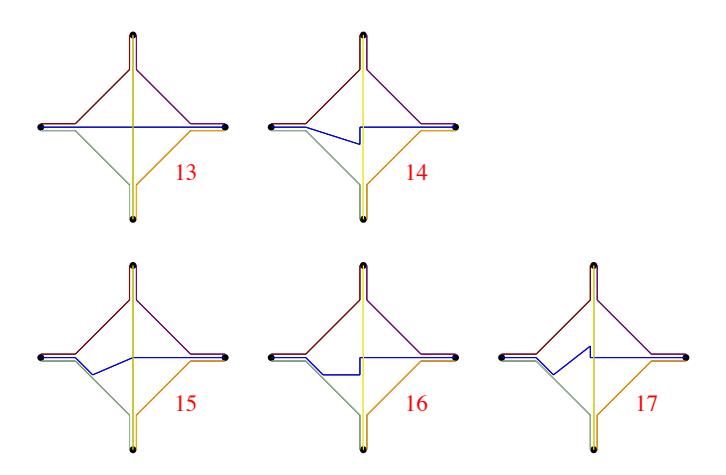
Figure 7. Types 13 - 17.
3.3. Degrees (4,4,3,3)
Next is the case where two of the four leaf-junctions have degree 4 and the other two have degree 3. This splits into two sub-cases. In the first sub-case the degree-4 vertices are opposite, say j-N and j-S. In this case, shown in Figure 8, the N-S route is again drawn in yellow and we need to consider where the E-W (drawn in blue) route might go. If these routes cross at a degree-4 vertex, the network must be type 18 or 19. If they share an edge, the network must be type 20 - 22.
Here types 21 and 22 are not isomorphic because, intuitively, the only possible homeomorphism would be a half-turn, but that takes each of those types to itself. Symbolically, in type 21 the route across the interior is described by the turn sequence RLLRRL (in either direction) whereas in type 22 it is RLRLRL; these sequences are not equivalent under reversals and L ↔ R interchange. Such arguments are implicitly used throughout subsequent cases, and we do not give details.
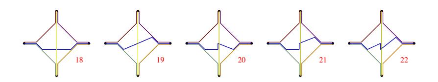
Figure 8. Types 18 - 22.
In the second sub-case the degree-4 leaf-junctions are adjacent, say j-N and j-E. here we find the eleven network types shown in Figure 9. Consider the two diagonal (N-S and E-W) routes. The rows in Figure 9 correspond to the cases
- (a) these routes cross in the interior of the diamond
- (b) these routes share an edge, but only in the strict interior of the diamond;
- (c) these routes coincide at some point on the boundary of the diamond.
And case (b) splits into the sub-case (b+) where the routes, directed away from the degree-4 leafjunctions, have the same direction on the shared edge, and the sub-case (b-) where they have opposite directions.
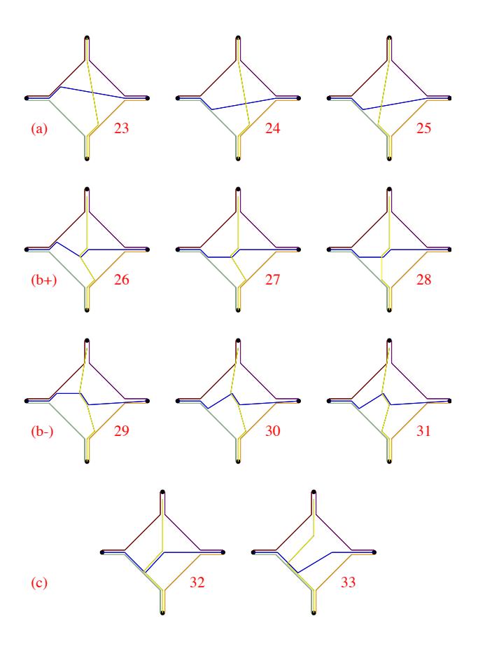
Figure 9. Types 23 - 33.
3.4. Degrees (4,3,3,3)
Next is the case where one of the four leaf-junctions has degree 4 and the other three have degree 3. This turns out to be simple to categorize. We may take the degree-4 junction as j-N, and may take the N-S route to meet the SE side of the diamond. Once this is done, the four sides of the diamond are distinguishable, and so we have 4 distinct possibilities for which sides of the diamonds are met by the E-W route. We then obtain the 12 types shown in the top 3 rows of Figure 10, where the three rows correspond to the 3 possibilities of the E-W route either crossing the N-S route, or sharing an edge in the N-S direction, or sharing an edge in the S-N direction – all this in the strict interior of the diamond.
The bottom two rows are the cases where these routes coincide at some point on the boundary of the diamond.
3.5. Degrees (3,3,3,3)
What remains is the case where all leaf-junctions have degree 3. In other words, from each starting point of each route between opposite leaves, the route starts along one edge of the diamond and then branches off. We will organize these networks via the numbers of such branchpoints on each diamond edge. Up to cyclic re-order and reversal there are four possibilities for the numbers of branchpoints on each diamond edge:
\[(1,1,1,1)\] \((2,1,0,1)\) \((2,1,1,0)\) \((2,0,2,0)\).
The corresponding networks are shown in Figure 11.
Figure 10. Types 34 - 51.
Figure 11. Types 52 - 71.
4. Coarser groupings
Our notion of topological isomorphism is a stringent requirement, and the resulting number (71) of types may be larger than one might wish for practical study of the "shape" of a network. Let us briefly consider two coarser classifications. Writing
F = number of inner faces
V = number of vertices, other than the 4 leaves
E = number of edges, other than the edges at leaves
Euler's formula tells us that E = F +V −1. So we could classify networks by values of (F, V, E). Alternatively we could classify by values of (f4, f3, f2, f1) where
fi := number of edges traversed by exactly i routes
again excluding edges at leaves.
| F | V | E | Types | f4 | f3 | f2 | f1 |
|---|---|---|---|---|---|---|---|
| 0 | 1 | 0 | 1 | ||||
| 0 | 2 | 1 | 2 | 1 | |||
| 1 | 3 | 3 | 5 | 2 | 1 | ||
| 1 | 4 | 4 | 3 | 1 | 2 | 1 | |
| 7 | 1 | 2 | 1 | ||||
| 1 | 5 | 5 | 6 | 4 | 2 | ||
| 2 | 4 | 5 | 8 | 2 | 3 | ||
| 2 | 5 | 6 | 9 | 1 | 2 | 3 | |
| 10 | 3 | 3 | |||||
| 2 | 6 | 7 | 4 | 1 | 4 | 2 | |
| 69 | 1 | 4 | 2 | ||||
| 11-12 | 1 | 3 | 3 | ||||
| 3 | 6 | 8 | 32-33 47 50 | 3 | 5 | ||
| 3 | 7 | 9 | 48 51 | 1 | 3 | 5 | |
| 46 49 55 61 67 | 4 | 5 | |||||
| 3 | 8 | 10 | 54 60 66 | 1 | 4 | 5 | |
| 56 62 68 | 5 | 5 | |||||
| 4 | 5 | 8 | 13 | 8 | |||
| 4 | 6 | 9 | 14-15 | 1 | 8 | ||
| 4 | 7 | 10 | 16-19 23-25 | 2 | 8 | ||
| 4 | 8 | 11 | 20-22 26-31 34-37 | 3 | 8 | ||
| 4 | 9 | 12 | 38-45 52 57 63 70 | 4 | 8 | ||
| 4 | 10 | 13 | 53 58-59 64-65 71 | 5 | 8 |
The table shows that for k = 4 the "Euler" categorization gives 17 types, and the "edgefrequency" categorization is a slight refinement that gives 23 types.
Implicit in our section 1.2 set-up is the fact that isomorphism of routed networks is a stronger property than isomorphism (in both cases, a graph isomorphism induced by a homeomorphism
from the plane R 2 to itself) of the underlying un-routed plane graphs. In the setting of our atlas of routed 4-networks satisfying (C3); the distinction is small, in that there are only three cases (shown in Figure 12) where two different types of routed network have isomorphic unrouted networks.
Figure 12. The three pairs of types whose unrouted networks are isomorphic: 9/10, 12/69 and 56/62.
Note here the two diagrams labelled 62 are in fact the same type.
5. Simulations and data
5.1. Simulations from SIRSN models
Let us recall very briefly the model from [3, 2]. Start with a square grid of roads, but impose a binary hierarchy of speeds: on a road meeting an axis at (2i + 1)2s , one can travel at speed γ −s for a parameter 1/2 < γ < 1. Define the route between grid points to be a shortest-time path. Then extend the construction to the continuum by including lines with s < 0.
Qualitatively, for γ near 1/2 one expects routes will exploit the "fast freeway" edges even when this involves longer route-length; whereas for γ near 1 routes will be shorter and use a greater variety of different edges.
The data below is from 100 simulations with the values γ = 0.6, 0.75, 0.9. The positions of the 4 leaves, in a square configuration, were randomly rotated and translated; recall that the essence of scale-invariance is that the size of the square makes no difference. The data was obtained from simulations without showing routes explicitly, so we could not reliably distinguish between the unrouted-isomorphic pairs in Figure 12, which ironically occurred quite often. Only a few of the simulated subnetworks, indicated by *, did not satisfy condition (C3).
\[\begin{split} \gamma &= 0.6 \text{ type} & 7 \quad 12/69 \quad 11 \quad 60 \quad * \\ \text{frequency} & 63 \quad 22 \quad 11 \quad 1 \quad 3 \end{split}\] \[\text{[rumus tidak dapat ditampilkan dengan baik — lihat PDF asli]}\] \[\text{[rumus tidak dapat ditampilkan dengan baik — lihat PDF asli]}\]
\[\gamma = 0.9 \ {\rm type} \quad 65 \quad 14 \quad 16 \quad 17 \quad 28 \quad 39 \quad 42 \quad 54 \quad 59 \quad 64 \quad * \\ {\rm frequency} \quad 2 \quad 1 \quad 1 \quad 1 \quad 1 \quad 1 \quad 1 \quad 1 \quad 1 \quad 3\]
The most common types were the simple networks shown in Figure 13.
Figure 13. Frequent types: 7, 12/69, 56/62 in the binary hierarchy model.
This data seems consistent with the qualitative behavior mentioned above. But in this model all edges are on a (rotated) square grid, so it is not a plausible representative of real-world road networks outside U.S. cities.
5.2. A little data from the U.S. road network
We sampled 30 subnetworks, each on 4 street addresses roughly in a square configuration, of sides between 50 and 250 miles. The frequencies of different types are shown here. Six types appeared more than once (frequency in parentheses)
\[7(4), 10(2), 11(4), 57(2), 59(3), 63(3)\]
and twelve types appeared exactly once
23, 24, 36, 39, 46, 52, 56, 60, 61, 66, 68, 70.
We see a larger diversity of types than in the particular SIRSN model in section 5.1; in particular the most frequent types in that model (Figure 14) are not so common in the real road network data, and indeed it seems intuitively clear they are artifacts of that specific model.
A serious statistical study of real road network data would present substantial conceptual and practical difficulties, and we do not attempt to do so here.
6. Remarks and open problems
Both the derivation of the classification and its uninformative organization as "types 1–71" are ad hoc and special to the case k = 4 and restriction (C3). Moreover for larger k the restriction (C3) seems less sensible. So
Problem 1. Give a rigorous classification of topological isomorphism classes of routed k-networks for general k ≥ 4, and an algorithm for deciding whether two given routed plane (i.e. embedded) networks are isomorphic.
Figure 12 showed that the type of a routed plane network is not determined by the (topological isomorphism) type of its plane graph (i.e. without specified routes). This prompts
Problem 2. Which (topological isomorphism types of) plane graph with k leaves arise from routed k-networks?
Thinking of routes as minimum-distance or minimum-time paths suggests the variants of the following problem.
Problem 3. Which routed k-networks can be embedded into the plane in such a way that routes are shortest-length paths, where the length of an edge (v1, v2) is
- (i) Euclidean distance;
- (ii) an arbitrary positive real number, subject to the "metric" constraint that it is at most the length of any alternate path from v1 to v2;
- (iii) an arbitrary positive real number.
We observed, from the table in section 4, that for k = 4 the "edge-frequency" categorization is a refinement of the "Euler" categorization. We conjecture this is not true for general k. That is, we conjecture that the implication
if two routed k-networks have the same frequencies (fi , i ≥ 1) of "number of edges traversed by exactly i routes" (and therefore the same number of edges) then they have the same number of vertices
is not true for large k.
Returning to the discussion of random networks in section 1.1, one can ask what probability distributions on types of routed 4-networks could arise from some SIRSN model (as the spanning subnetwork of 4 points in a square configuration). This question may be impossibly difficult. Problems like this are not well understood even in the setting of abstract (non-spatial) graphs. That is, the problem
what probability distributions µ on the set of graphs on 4 vertices arise as n → ∞ limits of the subgraphs of some n-vertex graph Gn sampled at 4 uniform random vertices
is in principle answered by the theory of graphons [10]: each graphon (a function W : [0, 1]2 → [0, 1]) determines some µW by a simple formula, and the set M in question is the set of all such µW . But this does not explicitly tell us whether a given µ is in M.
Acknowledgement
I thank Karthik Ganesan for the simulations of the SIRSN model in section 5.1, and Russell Mays for collecting the map data used in section 5.2. Research supported by NSF Grant DMS-1504802.
Answer: types in Figure 13. Left to right: types 71, 51, 65.
References
- [1] D. Aldous, The continuum random tree. II. An overview. In Stochastic analysis (Durham, 1990), volume 167 of London Math. Soc. Lecture Note Ser. (1991), pages 23–70, Cambridge Univ. Press, Cambridge.
- [2] D. Aldous, Scale-invariant random spatial networks, Electron. J. Probab. 19 (15) (2014), 1–41.
- [3] D. Aldous and K. Ganesan, True scale-invariant random spatial networks, Proc. Natl. Acad. Sci. USA 110 (22) (2013), 8782–8785.
- [4] D. Aldous, More uses of exchangeability: representations of complex random structures. In Probability and mathematical genetics, volume 378 of London Math. Soc. Lecture Note Ser. (2010), pages 35–63. Cambridge Univ. Press, Cambridge.
- [5] M. Barthelemy, Spatial networks, ´ Physics Reports 499 (2010), 1–101.
- [6] R. Diestel. Graph theory, volume 173 of Graduate Texts in Mathematics (1997), Springer-Verlag, New York. Translated from the 1996 German original.
- [7] E. Estrada, The Structure of Complex Networks: Theory and Applications (2011), Oxford University Press.
- [8] S. Janson, T. Łuczak and A. Rucinski, Random graphs (2000), Wiley-Interscience Series in Discrete Mathematics and Optimization, Wiley-Interscience, New York.
- [9] W. S. Kendall. From Random Lines to Metric Spaces. ArXiv e-print 1403.1156, 2014.
- [10] L. Lovasz, ´ Large networks and graph limits , volume 60 of American Mathematical Society Colloquium Publications (2012), American Mathematical Society, Providence, RI.
- [11] R. Milo, S. Shen-Orr, S. Itzkovitz, N. Kashtan, D. Chklovskii and U. Alon, Network motifs: Simple building blocks of complex networks, Science 298 (2002), 824–827.
- [12] M. E. J. Newman, The structure and function of complex networks, SIAM Rev. 45 (2003), 167–256 (electronic).
- [13] H. Towsner, Limits of Sequences of Markov Chains, Electron. J. Probab. 20 (77) (2015), 1–23.
Appendix A. Outline proof of Lemma 2.1.
Consider the union \((\tilde{G}, \text{say})\) of the 4 routes \(\text{route}(\ell_1, \ell_2)\), \(\text{route}(\ell_2, \ell_3)\), \(\text{route}(\ell_3, \ell_4)\), \(\text{route}(\ell_4, \ell_1)\) between adjacent leaves. There are a number of topologically different possibilities for \(\tilde{G}\) (ultimately the 7 shown in Figure 3, though we do not know that \(a\ priori\)) but the argument is essentially the same in every \(a\ priori\) possible case, so let us take the case of the diamond configuration shown in Figure 5.
We need to show that the N-S route does not go outside \(\tilde{G}\). Suppose it did. Then we can find a first-exit point \(x_1\) and a re-entry point \(x_2\) in \(\tilde{G}\), hence in at least one of the 4 routes (N-E, E-S. S-W, W-N) defining \(\tilde{G}\). These points cannot both be in the same defining route, by the consistency property (C2). But if they were in different defining routes, say N-E and E-S, then the intervening sub-route of the N-S route would need to loop around leaf E, or around leaves N, W, S, contradicting property (C3). The same contradiction arises for any distinct pair of defining routes.