Richard M. Lowa , W.H. Chanb
aDepartment of Mathematics, San Jose State University San Jose, CA 95192, USA
richard.low@sjsu.edu, waihchan@ied.edu.hk
The combinatorial game of Nim can be played on graphs. Over the years, various Nim-like games on graphs have been proposed and studied by N.J. Calkin et al., L.A. Erickson and M. Fukuyama. In this paper, we focus on the version of Nim played on graphs which was introduced by N.J. Calkin et al.: Two players alternate turns, each time choosing a vertex v of a finite graph and removing any number (≥ 1) of edges incident to v. The player who cannot make a move loses the game. Here, we analyze Graph Nim for various classes of graphs and also compute some Grundy-values.
Keywords: Nim on graphs, combinatorial game Mathematics Subject Classification : 05C57, 91A43, 91A46 DOI:10.5614/ejgta.2016.4.2.7
1. Introduction and some preliminaries
Having its humble beginnings in the context of recreational mathematics, combinatorial game theory has matured into an active area of research. Along with its natural appeal, the subject has applications to complexity theory, logic, graph theory and biology. For these reasons, combinatorial games have caught the attention of many people and the large body of research literature on the subject continues to increase. The interested reader is directed to [1, 2, 3, 7, 13, 14, 15], and to A. Fraenkel's excellent bibliography [10].
Received: 8 October 2015, Revised: 18 September 2016, Accepted: 29 September 2016.
bDepartment of Mathematics and Information Technology, The Hong Kong Institute of Education 10 Lo Ping Road, Tai Po, New Territories, Hong Kong
A combinatorial game is one of complete information and no element of chance is involved in gameplay. Each player is aware of the game position at any point in the game. Under normal play, two players alternate taking turns and a player loses when he cannot make a move. An impartial combinatorial game is one where both players have the same options from any position. A finite game eventually terminates (with a winner and a loser, no draws allowed).
Perhaps the most famous finite impartial combinatorial game is Nim, which is played in the following manner:
• There are n heaps, each containing a finite number of beads. Two players alternate turns, each time choosing a heap and removing any number (≥ 1) of beads in that heap. The player who cannot make a move loses the game.
In 1902, Bouton [4] gave a beautiful mathematical analysis and complete solution for Nim. Since then, the game of Nim has been the subject of many mathematics research papers.
Over the years, various Nim-like games on graphs have been proposed and studied [5, 9, 11, 12]. In this paper, we focus on the version of Nim played on graphs (called Graph Nim), introduced in [5]:
• Two players alternate turns, each time choosing a vertex v of a finite graph and removing any number (≥ 1) of edges incident to v. The player who cannot make a move loses the game.
Graph Nim is another example of a finite impartial combinatorial game (with normal play). In this paper, we will use some basic ideas and standard notation from combinatorial game theory, as found in [2], in the analysis of Graph Nim. For a more complete overview, the interested reader is directed to [2, 3, 7].
First, we recall a few definitions and some basic concepts from CGT.
Definition. A P-position is a position which is winning for the previous player (who has just moved). An N-position is a position which is winning for the next player (who is about to make a move).
In finite impartial combinatorial games (under normal play), P-positions and N-positions have the following properties:
- All terminal positions are P-positions.
- From every N-position, there is a move leading to a P-position.
- From every P-position, every move leads to an N-position.
The disjunctive sum of two or more game positions is the position obtained by placing the game positions side by side. When it is your move, you can make a single move in a summand of your choice. Note the following facts:
• The disjunctive sum of two P-positions is a P-position.
- The disjunctive sum of a P-position and an N-position is an N-position.
- The disjunctive sum of two N-positions is indeterminate.
- A game Γ equals 0 = {|} ⇐⇒ Γ is a P-position.
2. Results for various classes of graphs
Standard notation and definitions in graph theory, as found in [6], will be used in this paper. In [5], paths, cycles and complete graphs of order n, where 4 ≤ n ≤ 7, were analyzed. For the sake of completeness, we list these results in Theorems A–D.
Theorem A. Graph Nim played on Pn (of order n) is an N-position, for n ≥ 2.
Theorem B. Graph Nim played on Cn is a P-position, for n ≥ 3.
Theorem C. Graph Nim played on K2n is an N-position, for 1 ≤ n ≤ 6. Graph Nim played on K2m+1 is a P-position, for 1 ≤ m ≤ 5.
Theorem D. There exist arbitrarily large n, for which Graph Nim played on Kn is an N-position.
Proof. (Indirect). Assume that {Kn1 , Kn2 , . . . , Knr } (where n1 < n2 < · · · < nr) is the set of Ks, where the first-player wins. Then, Knr+1 is a second-player win (ie. a P-position). By Proposition 2.1, we have that Knr+2 is an N-position. This gives the desired contradiction and thus the claim is established.
Proposition 2.1. If there exists a vertex v of a graph G and a non-empty subset E = {vu1, vu2, . . . , vun} of E(G) such that Graph Nim played on G − E is a P-position, then Graph Nim played on G is an N-position.
Proof. Suppose that v is a vertex of G and E = {vu1, vu2, . . . , vun} is a non-empty subset of E(G) such that G − E is a P-position. The first-player removes all of the edges of E. The secondplayer must now make a move on G − E, a P-position. Thus, G is an N-position.
Let n ≥ 3. The wheel graph Wn (of order n + 1) is formed by adjoining a single vertex to all of the vertices on an n-cycle. The fan graph Fn (of order n + 1) is formed by removing a single non-spoke edge from Wn. The friendship graphs F Gn were characterized by Erdos et al. [8] and are isomorphic to Wn with a 1-factor removed from the outer-cycle.
Corollary 2.1. Let n ≥ 3. Then, Graph Nim played on Wn is an N-position.
Proof. Let n ≥ 3. Suppose the central edges (adjacent to vertex v) of Wn are e1, e2, . . . , en. Then, Wn−{e1, e2, . . . , en} = Cn∪{v}, which is a P-position by Theorem B. Thus, Wn is an N-position, by Proposition 2.1.
Corollary 2.2. Let n ≥ 3. Then, Graph Nim played on Fn is an N-position.
Proof. Let \(n \geq 3\). There exist edges \(e_1, e_2, \ldots, e_{n-2}\) (adjacent to vertex v) of \(F_n\) such that \(F_n - \{e_1, e_2, \ldots, e_{n-2}\} = C_{n+1}\), which is a P-position by Theorem B. Thus, \(F_n\) is an N-position, by Proposition 2.1.
Corollary 2.3. Let \(n \geq 4\). Then, Graph Nim played on \(FG_n\) is an N-position.
Proof. Because of the characterization of \(FG_n\) by Erdos et al. [8], we have that \(n \in \{4, 6, 8, \dots\}\). Suppose the central edges (adjacent to v) of \(FG_n\) are \(e_1, e_2, \dots, e_n\).
- (Case 1): \(n \equiv 0 \pmod{4}\). Then, \(FG_n \{e_1, e_2, \dots, e_n\} = (\frac{n}{2})P_2 \cup N_1 = (2r)P_2 \cup N_1\), namely 2r copies of \(P_2\) and an isolated vertex. This is clearly a P-position. Hence in this case, \(FG_n\) is an N-position by Proposition 2.1.
- (Case 2): \(n \equiv 2 \pmod{4}\). There exist central edges \(e_1, e_2, \ldots, e_{n-2}\) of \(FG_n\) such that \(FG_n \{e_1, e_2, \ldots, e_{n-2}\} = C_3 \cup (2s)P_2\), namely a \(C_3\) and 2s copies of \(P_2\). This is clearly a P-position, since \(C_3\) is a P-position by Theorem B and \((2s)P_2\) is a P-position. Hence in this case, \(FG_n\) is an N-position by Proposition 2.1.
Definition. Let \(r \ge 1\). A graph G of order 2r is 2-subgraph symmetric, if
- 1. G contains two vertex-disjoint isomorphic subgraphs \(G_1\) and \(G_2\), where \(V(G_1) = \{v_1, v_2, \dots, v_r\}\) and \(V(G_2) = \{u_1, u_2, \dots, u_r\}\), with \(v_i\) corresponding (under the subgraph isomorphism) to \(u_i\) for all i; and
- 2. \(v_i u_i \in E(G) \iff u_i v_i \in E(G)\).
Furthermore, if \(v_i u_i \notin E(G)\) for all i, then G is said to be restricted 2-subgraph symmetric.
Examples.
- 1. All \(C_{2r}\) are restricted 2-subgraph symmetric, for \(r \geq 2\).
- 2. All complete multipartite graphs \(K_{2r_1,2r_2,...,2r_k}\) are restricted 2-subgraph symmetric, for \(k \ge 2\). For example, see Figure 1.
- 3. Let M be a perfect matching of \(K_{2r}\), for \(r \ge 1\). Then, \(K_{2r} M\) is restricted 2-subgraph symmetric, while \(K_{2r}\) is 2-subgraph symmetric.
- 4. All \(P_{2r}\) are 2-subgraph symmetric, for \(r \geq 1\).
Theorem 5. Let G be restricted 2-subgraph symmetric. Then, Graph Nim played on G is a P-position.
Proof. Suppose some edges \(v_i v_j\) and \(v_i u_k\) (for a particular i) have been removed by the first-player. Edges \(u_i u_j\) and \(u_i v_k\) must still be in the graph and the second-player responds by removing them. The remaining graph is again restricted 2-subgraph symmetric. This process is repeated until the last edge(s) is removed by the second-player.
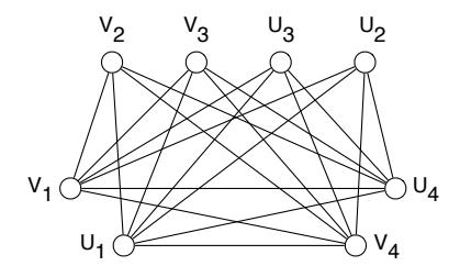
Figure 1. K4,2,2 is restricted 2-subgraph symmetric.
Corollary 2.4. Let M be a perfect matching of K2r, with r ≥ 2. Then, Graph Nim played on K2r − M is a P-position.
Corollary 2.5. Let M be a maximum matching of K2r+1 with r ≥ 2. Then, Graph Nim played on K2r+1 − M is an N-position.
Proof. This follows immediately from Corollary 2.4 and Proposition 2.1.
Corollary 2.6. Let n1, n2, . . . , nk ∈ 2N and k ≥ 2. Then, Graph Nim played on Kn1,n2,...,nk is a P-position.
Corollary 2.7. Let n1, n2, . . . , nk−1 ∈ 2N, k ≥ 2, and nk be odd. Then, Graph Nim played on Kn1,n2,...,nk is an N-position.
Proof. This follows immediately from Corollary 2.6 and Proposition 2.1.
Remark. Note that a 2-subgraph symmetric graph might be an N-position or a P-position. Both graphs in Figure 2 are 2-subgraph symmetric. The path P4 in Figure 2 is an N-position, In contrast, the graph on the right in Figure 2 is a P-position. For the second graph, one can show this directly by analyzing the eight distinct game positions which can arise after the first-player makes his first move.
Figure 2. A 2-subgraph symmetric graph can be an N-position or a P-position.
Recall the definition of the line graph L(G), for a simple graph G.
Definition. Let G be a simple graph with p vertices and q edges. The line graph of G, denoted by L(G), is the graph where V (L(G)) = {v1, v2, . . . , vq} and vivj ∈ E(L(G)) if and only if edges ei and ej are incident in G.
Lemma 2.1. Let G be restricted 2-subgraph symmetric. Then, L(G) is restricted 2-subgraph symmetric and hence, a P-position for G-properties.
Proof. Since G is restricted 2-subgraph symmetric, there exists a partition of V(G); \(V_1(G) =\)\(\{v_1, v_2, \dots, v_r\}\) and \(V_2(G) = \{u_1, u_2, \dots, u_r\}\), such that the induced subgraphs (of the vertex sets) are isomorphic (with \(v_i \leftrightarrow u_i\)), \(v_i u_i \notin E(G)\) for all i, and \(v_i u_i \in E(G) \Leftrightarrow u_i v_i \in E(G)\). Let \(\langle V_i(G) \rangle\) denote the subgraph induced by \(V_i(G)\), for i = 1, 2. Clearly, \(L(\langle V_1(G) \rangle) \cong L(\langle V_2(G) \rangle)\). Let \(L(\langle V_1(G) \rangle) = \{\overline{v}_1, \overline{v}_2, \dots, \overline{v}_k\}\) and \(L(\langle V_2(G) \rangle) = \{\overline{u}_1, \overline{u}_2, \dots, \overline{u}_k\}\). Note that V(L(G)) may contain vertices which don't belong to \(V(L(\langle V_1(G)\rangle)) \cup V(L(\langle V_2(G)\rangle))\). In particular, these vertices tices \(s_1, s_2, \ldots, s_m, t_1, t_2, \ldots, t_m\) correspond to edges \(u_i v_j \in E(G)\). Let \(\mathcal{S} = \{u_i v_j \in E(G) : i < i\}\)j} and \(\mathcal{T} = \{u_i v_i \in E(G) : i > j\}\). The vertices \(s_1, s_2, \ldots, s_m\) in V(L(G)), corresponding to edges in S, can be ordered in the following way: \(u_i v_i < u_c v_d \iff i < c \text{ or } (i = c \text{ and } j < d)\). Using this, set \(S' = \{s_1, s_2, \dots, s_m\}\). This induces an ordering of the vertices \(t_1, t_2, \dots, t_m\) in V(L(G)), corresponding to edges in \(\mathcal{T}\), in the following way: If \(s_l \leftrightarrow u_i v_j\), then \(t_l \leftrightarrow v_i u_j\). Using this, set \(\mathcal{T}' = \{t_1, t_2, \dots, t_m\}\). Notice that edges \(s_l t_l\) do not exist in L(G), since edges \(u_i v_j\) and \(v_i u_j\)are disjoint in G. Also, edges \(\overline{v}_l \overline{u}_l\) do not exist in L(G), since the edge (corresponding to \(\overline{v}_l\)) and the edge (corresponding to \(\overline{u}_l\)) in G are not adjacent. Finally, let \(V_1' = \{\overline{v}_1, \overline{v}_2, \dots, \overline{v}_k, s_1, s_2, \dots, s_m\}\)and \(V_2' = \{\overline{u}_1, \overline{u}_2, \dots, \overline{u}_k, t_1, t_2, \dots, t_m\}\), with correspondences \(\overline{v}_i \leftrightarrow \overline{u}_i\) and \(\overline{s}_i \leftrightarrow \overline{t}_i\). This partition of V(L(G)) implies that L(G) is restricted 2-subgraph symmetric. Hence, Graph Nim played on L(G) is a P-position, by Theorem 5.
Corollary 2.8. Let G be restricted 2-subgraph symmetric. Then, Graph Nim played on \(L(L \cdots L(G))\) is a P-position.
Proof. This follows immediately from Lemma 2.1 and Theorem 5.
In Figure 3, the graph G on the left is restricted 2-subgraph symmetric. The graph on the right is L(G), which is also restricted 2-subgraph symmetric. Hence, they are both P-positions.
Remark. Note that the converse of Lemma 2.1 is not necessarily true. For example, \(L(K_4) \cong K_{2,2,2}\) (the octahedral graph), which is restricted 2-subgraph symmetric. However, \(K_4\) is 2-subgraph symmetric. On the other hand, the converse of Lemma 2.1 is sometimes true. For example, \(L(C_{2r}) \cong C_{2r}\) for \(r \geq 2\), which is restricted 2-subgraph symmetric.
Now, let us recall the definition of the Cartesian product of graphs \(G_1\) and \(G_2\).
Definition. Given graphs \(G_1\) and \(G_2\), the Cartesian product of \(G_1\) and \(G_2\) (denoted by \(G_1 \times G_2\)) is the graph, where \(V(G_1 \times G_2) = V_1 \times V_2 = \{(a,b) : a \in V_1 \land b \in V_2\}\) and \(E(G_1 \times G_2) = \{((a,b),(a',b')) : a,a' \in V_1 \land b,b' \in V_2 \land ((a=a' \land (b,b') \in E_2) \lor (b=b' \land (a,a') \in E_1))\}.\)
Theorem 6. Let G be a graph and G' be restricted 2-subgraph symmetric. Then, \(G \times G'\) is restricted 2-subgraph symmetric and hence, is a P-position for Graph Nim.
Proof. Suppose G (a graph) and G' (restricted 2-subgraph symmetric) are of orders n and 2r, respectively. Let \(G'_A\) and \(G'_B\) be the two isomorphic subgraphs of G' (as found in the definition
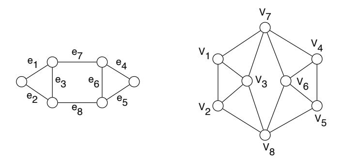
Figure 3. Graph G and its line graph L(G).
of 2-subgraph symmetric). Let \(G_i'\) be a copy of G' in \(G \times G'\), \(1 \leq i \leq n\), and \(G_{i,A}'\) and \(G_{i,B}'\) be the two isomorphic subgraphs of \(G_i'\) with \(V(G_{i,A}') = \{v_{i,A,1}, v_{i,A,2}, \ldots, v_{i,A,r}\}\), \(V(G_{i,B}') = \{v_{i,B,1}, v_{i,B,2}, \ldots, v_{i,B,r}\}\), and \(v_{i,A,j}\) corresponding (under the isomorphism) to \(v_{i,B,j}\), for all j. Clearly, \(G \times G_A'\) and \(G \times G_B'\) are vertex disjoint isomorphic subgraphs of \(G \times G'\), with \(V(G \times G_A') \cup V(G \times G_B') = V(G \times G')\). Let uw be an edge of \(G \times G'\), which is one of five possible types:
- \(u \in V(G'_{i,A})\) and \(w \in V(G'_{i,B})\), for some i.
- \(u, w \in V(G'_{i,A})\), for some i.
- \(u, w \in V(G'_{i,B})\), for some i.
- \(u \in V(G'_{i,A})\) and \(w \in V(G'_{j,A})\), where \(i \neq j\).
- \(u \in V(G'_{i,B})\) and \(w \in V(G'_{j,B})\), where \(i \neq j\).
For the first three types of edges, there exists an edge \(\overline{wu} \in E(G \times G')\), since \(G'_i\) is restricted 2-subgraph symmetric. In the last two types of edges, there exists an edge \(\overline{wu} \in E(G \times G')\), because of the definition of \(G \times G'\). Thus, \(G \times G'\) is restricted 2-subgraph symmetric. Hence, Graph Nim played on \(G \times G'\) is a P-position, by Theorem 5.
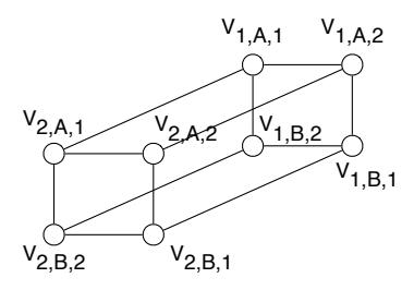
Figure 4. The Cartesian product of \(P_2\) and restricted 2-subgraph symmetric \(C_4\).
Remark. If G is a graph and G' is a P-position, then \(G \times G'\) is not necessarily a P-position. For example, let \(G = P_2\) and \(G' = C_3\), which is a P-position. Now, consider Graph Nim played on \(P_2 \times C_3\). The first-player can remove a single edge, leaving the second-player to move on the graph in Figure 5, which is a P-position. Thus, \(P_2 \times C_3\) is an N-position.
Figure 5. This graph is a P-position.
Theorem 7. Let G' and G'' be 2-subgraph symmetric. Then, \(G' \times G''\) is restricted 2-subgraph symmetric and hence, is a P-position for Graph Nim.
Proof. Let \(G_1'\) and \(G_2'\) be the isomorphic subgraphs of G', and \(G_1''\) and \(G_2''\) be the isomorphic subgraphs of G''. Then, \(G_1' \times G_1'' \cong G_2' \times G_1'' \cong G_1' \times G_2'' \cong G_2' \times G_2''\) with \(V(G_i' \times G_j'') = \{v_{i,j,l,m}: 1 \leq l \leq |V(G_i')| \text{ and } 1 \leq m \leq |V(G_j'')| \}\) for \(1 \leq i,j \leq 2\), and \(v_{1,1,l,m}, v_{2,1,l,m}, v_{1,2,l,m}\) and \(v_{2,2,l,m}\) all correspond to one another (under the isomorphisms), for all l and m (see Figure 6). For the isomorphism \(G_1' \times G'' \cong G_2' \times G''\), we associate vertices \(v_{1,1,l,m}\) and \(v_{1,2,l,m}\) (in \(G_1' \times G''\)) to vertices \(v_{2,2,l,m}\) and \(v_{2,1,l,m}\) (in \(G_2' \times G''\)), respectively. From the definition of the Cartesian product \(G' \times G''\), we have \(v_{i,j,l,m}v_{i',j',l',m'} \notin E(G' \times G'')\) for all l, l', m and m' when \(i \neq i'\) and \(j \neq j'\). Furthermore, since \(G' \times G_1''\) is isomorphic to \(G' \times G_2''\), we have \(v_{1,1,l,m}v_{2,1,l,m} \in E(G' \times G'')\) if and only if \(v_{1,2,l,m}v_{2,2,l,m} \in E(G' \times G'')\). Thus, \(G' \times G''\) is restricted 2-subgraph symmetric. Hence, Graph Nim played on \(G' \times G''\) is a P-position, by Theorem 5.
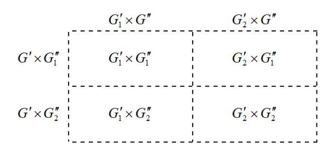
Figure 6. Structure of \(G' \times G''\).
Examples.
1. Let \(r, s \in \mathbb{N}\). Then, \(P_{2r} \times P_{2s}\), \(P_{2r} \times K_{2s}\) and \(K_{2r} \times K_{2s}\) are restricted 2-subgraph symmetric and hence P-positions, by Theorem 7.
2. Let G be a graph and \(r, s \in \mathbb{N}\). Then, \(G \times C_{2r}\), \(G \times P_{2r} \times P_{2s}\), \(G \times P_{2r} \times K_{2s}\) and \(G \times K_{2r} \times K_{2s}\) are restricted 2-subgraph symmetric and hence P-positions, by Theorems 6 and 7.
Corollary 2.9. Graph Nim played on the hypercube \(Q_n\) is a P-position, for all \(n \geq 2\).
Proof. Let \(n \ge 2\). Since \(Q_n = P_2 \times P_2 \times \cdots \times P_2\) (n factors), the result follows immediately from Theorems 7, 6, and 5.
Theorem 8. Let \(G = P_n \times P_m\) and \(m \ge 2\). If m and n are even, then Graph Nim played on G is a P-position. Otherwise, G is an N-position.
Proof. Let \(G = P_n \times P_m\). If n = 1, then \(G = P_m\) is an N-position. If both n and m are even, then \(P_n\) and \(P_m\) are 2-subgraph symmetric and hence, G is a P-position (by Theorems 7 and 5). We now consider the last case where \(n, m \ge 2\), with at least one of n, m being odd. Let \(V(G) = \{v_{i,j} : 1 \le i \le n \text{ and } 1 \le j \le m\}\) as shown in Figure 7. If n is even and m is odd, then \(G[\{v_{i,j}: 1 \le i \le \frac{n}{2} \text{ and } 1 \le j \le m\}]\) is isomorphic to \(G[\{v_{i,j}: \frac{n}{2}+1 \le i \le n \text{ and } 1 \le j \le m\}]\), with \(v_{i,j}\) corresponding to \(v_{n-i+1,m-j+1}\) for \(1 \le i \le \frac{n}{2}\) and \(1 \le j \le m\) (see Figure 7(a)). Hence, \(G - \{v_{\frac{n}{2},\lceil \frac{m}{2} \rceil}v_{\frac{n}{2}+1,\lceil \frac{m}{2} \rceil}\}\) is restricted 2-subgraph symmetric, a P-position by Theorem 5. Thus, G is an N-position by Proposition 2.1. If n is odd and m is even, then a similar vertexset partition and correspondence (see Figure 7(b)) shows that \(G - \{v_{\lceil \frac{n}{2} \rceil, \frac{m}{2}} v_{\lceil \frac{n}{2} \rceil, \frac{m}{2}+1}\}\) is restricted 2-subgraph symmetric, a P-position. Thus, G is an N-position. Lastly, suppose that n, m are both odd. Let \(\text{[rumus tidak dapat ditampilkan dengan baik — lihat PDF asli]}\) and \(\text{[rumus tidak dapat ditampilkan dengan baik — lihat PDF asli]}\) and \(V_2 = \{v_{i,j} : \lceil \frac{n}{2} \rceil + 1 \le i \le n \text{ and } 1 \le j \le m\} \cup \{v_{\lceil \frac{n}{2} \rceil, k} : \lceil \frac{m}{2} \rceil + 1 \le k \le m\}.\) Then, \(G[V_1]\) and \(G[V_2]\) are isomorphic with \(v_{i,j}\) corresponding to \(v_{n-i+1,m-j+1}\) for \(1 \leq i \leq \lfloor \frac{n}{2} \rfloor\) and \(1 \le j \le m\), and \(v_{\lceil \frac{n}{2} \rceil, j}\) corresponding to \(v_{\lceil \frac{n}{2} \rceil, m-j+1}\) for \(1 \le j \le \lfloor \frac{m}{2} \rfloor\) (see Figure 7(c)). Moreover, \(G - \{v_{\lceil \frac{n}{2} \rceil, \lceil \frac{m}{2} \rceil} v_{\lceil \frac{n}{2} \rceil, \lfloor \frac{m}{2} \rfloor}, v_{\lceil \frac{n}{2} \rceil, \lceil \frac{m}{2} \rceil} v_{\lceil \frac{n}{2} \rceil, \lceil \frac{m}{2} \rceil} v_{\lceil \frac{n}{2} \rceil, \lceil \frac{m}{2} \rceil} v_{\lfloor \frac{n}{2} \rfloor, \lceil \frac{m}{2} \rceil}, v_{\lceil \frac{n}{2} \rceil, \lceil \frac{m}{2} \rceil} v_{\lceil \frac{n}{2} \rceil, \lceil \frac{m}{2} \rceil} \}\) is restricted 2-subgraph symmetric (and hence, a P-position by Theorem 5). Thus, G is an N-position by Proposition 2.1.
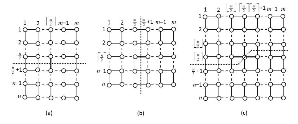
Figure 7. Vertex partitions which yield isomorphic subgraphs of \(P_n \times P_m\).
What can be said with regards to other types of graph products? Let us recall the following definitions.
Definition. Lexicographic product G1 • G2: V (G1 • G2) = V1 × V2 = {(a, b) : a ∈ V1 ∧ b ∈ V2} and E(G1 •G2) = {((a, b),(a 0 , b0 )) : a, a0 ∈ V1 ∧ b, b0 ∈ V2 ∧ ((a = a 0 ∧ (b, b0 ) ∈ E2) ∨ (a, a0 ) ∈ E1)}.
Definition. Tensor product G1 ⊗ G2: V (G1 ⊗ G2) = V1 × V2 = {(a, b) : a ∈ V1 ∧ b ∈ V2} and E(G1 ⊗ G2) = {((a, b),(a 0 , b0 )) : a, a0 ∈ V1 ∧ b, b0 ∈ V2 ∧ (a, a0 ) ∈ E1 ∧ (b, b0 ) ∈ E2}.
Of these two products, only the lexicographic product is not commutative.
Theorem 9. Let n ≥ 2 and Nm be the null graph of order m. If m is odd, then Graph Nim played on G = Pn • Nm is an N-position. Otherwise, G is a P-position.
Proof. If m and n are odd, the first-player should remove the dark edges in Figure 8(a) on his first move. This leaves a restricted 2-subgraph symmetric graph (a P-position) for the second-player to move from. However, if m is odd and n is even, the first-player should remove the dark edge in Figure 8(b) on his first move, which leaves a restricted 2-subgraph symmetric graph for the second-player to move from. In both of these cases, we see that G is an N-position. If m is even, then Figure 8(c) gives a vertex partition which illustrates that G is a P-position.
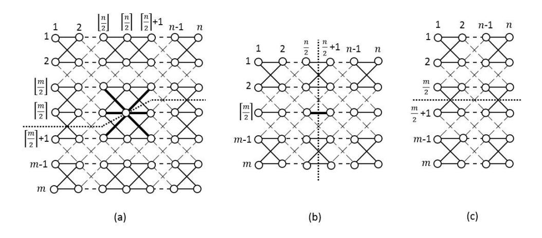
Figure 8. Vertex partitions which yield isomorphic subgraphs of Pn • Nm.
Theorem 10. Let m, n ≥ 2. If m and n are both odd, then Graph Nim played on G = Pm ⊗ Pn is an N-position. Otherwise, G is a P-position.
Proof. If m and n are odd, the first-player should remove the dark edges in Figure 10(a) on his first move. This leaves a restricted 2-subgraph symmetric graph (a P-position) for the second-player to
Figure 9. P4 • N2 is restricted 2-subgraph symmetric and thus, is a P-position.
move from. In this case, we see that G is an N-position. In the other cases, Figure 10(b) gives a vertex partition which illustrates that G is a P-position.
Figure 10. Vertex partitions which yield isomorphic subgraphs of Pm ⊗ Pn.
3. Grundy-values
Not surprisingly, the N- and P-positions (in Graph Nim) are highly dependent on the structure of the underlying graph. It is quite likely that general results cannot be obtained for Graph Nim. In this section, we use elementary combinatorial game theory to analyze some additional classes of graphs. Here, we do not focus on the technical details of CGT. The discussion below is merely an informal presentation of material arising from the Sprague-Grundy Theorem and CGT (as developed by Berlekamp, Conway, and Guy). The reader who is interested in the technical details is referred to [2, 3, 7]. Instead, we will briefly explain the relevant ideas and their applications to the analysis of Graph Nim.
For any finite impartial combinatorial game Γ, there is an associated value (Grundy-value) G(Γ). In this context, such values are called nimbers and they are denoted by ∗0 = 0, ∗1, ∗2, ∗3, . . . etc. (or 0, 1, 2, 3, . . . , etc., when there's no possibility for confusion). The Grundy-value G(Γ) immediately tells us if Γ is a P-position or an N-position. In particular, G(Γ) = 0 ⇐⇒ Γ is a P-position. To compute G(Γ), we need the following two definitions.
Figure 11. P4 ⊗ P4 is restricted 2-subgraph symmetric and thus, is a P-position.
Definition. The minimum excluded value (or mex) of a set of non-negative integers is the smallest non-negative integer which does not occur in the set. This is denoted by mex{a, b, c, . . . , k}.
Definition. Let Γ be a finite impartial game. Then,
\[\mathcal{G}(\Gamma) = \max{\{\mathcal{G}(\Delta) : \Delta \text{ is an option of } \Gamma\}}.\]
For any finite impartial game Γ which is a disjunctive sum of finite impartial games γ1 +γ2 +· · ·+ γk, G(Γ) = PG(γi), where the sum is BitXor (Nim-addition).
Lemma 3.1. Let n ≥ 1. Then, G(K1,n) = ∗n.
Proof. This follows immediately from a straightforward induction argument.
In an attempt to gain deeper insight into Graph Nim, we created some Mathematica programs to compute the Grundy-values for some classes of graphs. In [5], the Grundy-values for paths were computed. The values have been confirmed by the authors of this paper and we list them in Figure 12 for quick reference. The (ij)th-entry in the table denotes the Grundy-value for P12(i−1)+j . Note that the Grundy-values become periodic (rows 7, 8, . . . are identical). We then use this to compute the Grundy-values for certain classes of broom graphs Bn,k. This, in turn, will allow us to construct infinite classes of N-position double-broom graphs DBj,n,k.
Definition. A broom graph Bn,k is a path of n vertices, with k (≥ 2) pendant edges attached to an end-vertex. A double-broom graph DBj,n,k is a path of n vertices, with j (≥ 2) pendant edges attached to an end-vertex and k (≥ 2) pendant edges attached to the other end-vertex.
The Grundy-values for Bn,2 were also computed in [5]. These values have been confirmed by the authors of this paper and we list them in Figure 13. There, the (ij)th-entry in the table denotes the Grundy-value for B12(i−1)+j,2. Note that the Grundy-values become periodic (rows 14, 15, . . . are identical).
| 1 | 2 | 3 | 4 | 5 | 6 | 7 | 8 | 9 | 10 | 11 | 12 | |
|---|---|---|---|---|---|---|---|---|---|---|---|---|
| 1 | 0 | 1 | 2 | 3 | 1 | 4 | 3 | 2 | 1 | 4 | 2 | 6 |
| 2 | 4 | 1 | 2 | 7 | 1 | 4 | 3 | 2 | 1 | 4 | 6 | 7 |
| 3 | 4 | 1 | 2 | 8 | 5 | 4 | 7 | 2 | 1 | 8 | 6 | 7 |
| 4 | 4 | 1 | 2 | 3 | 1 | 4 | 7 | 2 | 1 | 8 | 2 | 7 |
| 5 | 4 | 1 | 2 | 8 | 1 | 4 | 7 | 2 | 1 | 4 | 2 | 7 |
| 6 | 4 | 1 | 2 | 8 | 1 | 4 | 7 | 2 | 1 | 8 | 6 | 7 |
| 7 | 4 | 1 | 2 | 8 | 1 | 4 | 7 | 2 | 1 | 8 | 2 | 7 |
| 8 | 4 | 1 | 2 | 8 | 1 | 4 | 7 | 2 | 1 | 8 | 2 | 7 |
| 9 | 4 | 1 | 2 | 8 | 1 | 4 | 7 | 2 | 1 | 8 | 2 | 7 |
| 10 | 4 | 1 | 2 | 8 | 1 | 4 | 7 | 2 | 1 | 8 | 2 | 7 |
Figure 12. Grundy-values for Pn.
| 1 | 2 | 3 | 4 | 5 | 6 | 7 | 8 | 9 | 10 | 11 | 12 | |
|---|---|---|---|---|---|---|---|---|---|---|---|---|
| 1 | 2 | 3 | 4 | 5 | 6 | 2 | 1 | 0 | 8 | 6 | 0 | 1 |
| 2 | 2 | 3 | 8 | 5 | 12 | 7 | 1 | 0 | 8 | 9 | 14 | 1 |
| 3 | 2 | 3 | 11 | 4 | 7 | 12 | 14 | 0 | 16 | 2 | 4 | 12 |
| 4 | 2 | 3 | 10 | 4 | 7 | 15 | 1 | 16 | 9 | 18 | 16 | 12 |
| 5 | 2 | 3 | 10 | 16 | 7 | 12 | 1 | 16 | 18 | 11 | 16 | 12 |
| 6 | 2 | 22 | 11 | 16 | 7 | 12 | 1 | 20 | 24 | 16 | 26 | 12 |
| 7 | 13 | 22 | 11 | 16 | 24 | 15 | 14 | 16 | 22 | 19 | 16 | 12 |
| 8 | 13 | 19 | 11 | 16 | 24 | 15 | 14 | 16 | 25 | 11 | 16 | 12 |
| 9 | 13 | 22 | 11 | 16 | 7 | 15 | 1 | 20 | 25 | 19 | 11 | 12 |
| 10 | 13 | 22 | 11 | 32 | 19 | 22 | 14 | 20 | 22 | 19 | 11 | 12 |
| 11 | 13 | 22 | 11 | 25 | 19 | 22 | 14 | 16 | 22 | 19 | 11 | 21 |
| 12 | 13 | 22 | 11 | 25 | 19 | 22 | 14 | 21 | 25 | 19 | 11 | 21 |
| 13 | 13 | 22 | 11 | 25 | 19 | 22 | 14 | 20 | 22 | 19 | 11 | 21 |
| 14 | 13 | 22 | 11 | 25 | 19 | 22 | 14 | 21 | 22 | 19 | 11 | 21 |
| 15 | 13 | 22 | 11 | 25 | 19 | 22 | 14 | 21 | 22 | 19 | 11 | 21 |
Figure 13. Grundy-values for Bn,2.
By computing the Grundy-values for Pn, K1,n, Bn,2, Bn,3, etc., we can identify many trees which are N-positions.
Examples.
- 1. The double-broom graph DB4,4,2, (i.e. P4, with 4 pendant edges on one end and 2 pendant edges on the other end) is an N-position. This is because the first-player can remove the single edge from the graph, leaving a K1,4 and a B3,2. The second-player must now move in a game position which has Grundy-value ∗4 + ∗4 = 0 (ie. BitXor, Nim-addition).
- 2. Suppose that T is a tree with the following property: There exists a vertex v such that the removal of some edges {ej} incident to v results in a disjoint collection of P2, B3,2 and K1,5 (ignoring isolated vertices). The Grundy-values of P2, B3,2 and K1,5 are 1, 4 and 5, respectively. This particular game position has Grundy-value ∗1 + ∗4 + ∗5 = 0. Thus, T is an N-position since the first-player merely removes edges {ej} from T, which leaves the
second-player to move in a game position having Grundy-value 0.
3. Consider the graph B8,2, which has Grundy-value 0. This means that it is a P-position. No matter what moves the first-player makes, the second-player can eventually win the game. Say for example, that the first-player removes two edges, leaving a P3 and a B4,2. This results in a game position with Grundy-value ∗2 + ∗5 = ∗7. The second-player can then remove three edges (from the B4,2 component), which leaves a game position with Grundy-value ∗2 + ∗2 = 0.
Definition. Let n ≥ 1. A tadpole graph Tn is a path of n vertices with a cycle C3 attached to an end-vertex.
Using Figures 12 and 13, we compute the Grundy-values for Tn. They are given in Figure 14. The (ij)th-entry in the table denotes the Grundy-value for T12(i−1)+j . Note that the Grundy-values become periodic (rows 13, 14, . . . are identical).
| 1 | 2 | 3 | 4 | 5 | 6 | 7 | 8 | 9 | 10 | 11 | 12 | |
|---|---|---|---|---|---|---|---|---|---|---|---|---|
| 1 | 0 | 4 | 2 | 6 | 7 | 4 | 3 | 7 | 1 | 8 | 9 | 6 |
| 2 | 11 | 1 | 12 | 7 | 10 | 4 | 8 | 10 | 11 | 4 | 9 | 16 |
| 3 | 14 | 1 | 12 | 7 | 14 | 1 | 13 | 2 | 1 | 4 | 13 | 2 |
| 4 | 14 | 1 | 2 | 7 | 10 | 4 | 8 | 2 | 10 | 16 | 13 | 7 |
| 5 | 11 | 1 | 16 | 7 | 14 | 4 | 8 | 2 | 11 | 4 | 13 | 7 |
| 6 | 14 | 1 | 16 | 7 | 18 | 4 | 13 | 2 | 11 | 4 | 13 | 16 |
| 7 | 14 | 1 | 16 | 7 | 18 | 4 | 13 | 20 | 10 | 4 | 13 | 7 |
| 8 | 14 | 1 | 20 | 7 | 18 | 4 | 8 | 20 | 11 | 4 | 13 | 7 |
| 9 | 14 | 1 | 20 | 7 | 18 | 4 | 13 | 2 | 11 | 4 | 13 | 7 |
| 10 | 14 | 1 | 20 | 7 | 18 | 4 | 13 | 22 | 11 | 4 | 13 | 7 |
| 11 | 14 | 1 | 20 | 7 | 18 | 4 | 13 | 25 | 11 | 4 | 13 | 7 |
| 12 | 14 | 1 | 20 | 7 | 18 | 4 | 13 | 20 | 11 | 4 | 13 | 7 |
| 13 | 14 | 1 | 20 | 7 | 18 | 4 | 13 | 25 | 11 | 4 | 13 | 7 |
| 14 | 14 | 1 | 20 | 7 | 18 | 4 | 13 | 25 | 11 | 4 | 13 | 7 |
| 15 | 14 | 1 | 20 | 7 | 18 | 4 | 13 | 25 | 11 | 4 | 13 | 7 |
Figure 14. Grundy-values for Tn.
Examples.
- 1. Consider the graph T6, which has Grundy-value ∗4. This indicates that Graph Nim played on T6 is an N-position. The first-player merely removes the single edge which leaves a T3 and P3. This resulting position has a Grundy-value of ∗2+∗2 = 0 (a losing position), from which the second-player must move. From this point on, whatever move the second-player makes, the first-player responds by removing edge(s) so that the resulting position has Grundy-value 0.
- 2. Let n ≥ 2. Then, Tn is an N-position, since G(Tn) 6= 0.
- 3. Suppose that G is a graph with the following property: There exists a vertex v such that the removal of some edges {ej} incident to v results in a disjoint union (having an even
number of components) of T3 and B6,2 (ignoring isolated vertices). The Grundy-values of T3 and B6,2 are the same, namely 2. This particular game position has Grundy-value ∗2+∗2+· · ·+∗2 = 0, since there is an even number of summands. Thus, G is an N-position since the first-player merely removes edges {ej} from G, which leaves the second-player to move in a game position having Grundy-value 0 (a losing position).
We can continue to compute Grundy-values for other classes of graphs. For example, by using Figures 12 and 13, we compute the Grundy-values for Bn,3. They are given in Figure 15. The (ij)th-entry in the table denotes the Grundy-value for B12(i−1)+j,3. Note that the Grundy-values become periodic (rows 13, 14, . . . are identical).
| 1 | 2 | 3 | 4 | 5 | 6 | 7 | 8 | 9 | 10 | 11 | 12 | |
|---|---|---|---|---|---|---|---|---|---|---|---|---|
| 1 | 3 | 4 | 5 | 6 | 7 | 5 | 0 | 8 | 6 | 5 | 1 | 8 |
| 2 | 3 | 10 | 5 | 6 | 3 | 10 | 0 | 8 | 6 | 10 | 0 | 2 |
| 3 | 3 | 10 | 5 | 9 | 12 | 1 | 0 | 8 | 6 | 10 | 15 | 2 |
| 4 | 3 | 10 | 5 | 6 | 16 | 14 | 18 | 8 | 6 | 5 | 18 | 13 |
| 5 | 3 | 10 | 5 | 6 | 15 | 10 | 18 | 8 | 6 | 5 | 12 | 9 |
| 6 | 3 | 10 | 5 | 6 | 15 | 10 | 18 | 8 | 6 | 4 | 15 | 9 |
| 7 | 3 | 10 | 18 | 17 | 15 | 10 | 18 | 8 | 17 | 18 | 12 | 13 |
| 8 | 3 | 10 | 18 | 12 | 15 | 10 | 18 | 8 | 6 | 18 | 12 | 9 |
| 9 | 3 | 10 | 5 | 6 | 15 | 10 | 18 | 8 | 6 | 5 | 12 | 9 |
| 10 | 3 | 10 | 18 | 17 | 15 | 10 | 18 | 8 | 17 | 18 | 12 | 9 |
| 11 | 3 | 10 | 18 | 12 | 15 | 10 | 18 | 8 | 17 | 18 | 12 | 9 |
| 12 | 3 | 10 | 18 | 12 | 15 | 10 | 18 | 8 | 6 | 18 | 12 | 9 |
| 13 | 3 | 10 | 18 | 12 | 15 | 10 | 18 | 8 | 17 | 18 | 12 | 9 |
| 14 | 3 | 10 | 18 | 12 | 15 | 10 | 18 | 8 | 17 | 18 | 12 | 9 |
| 15 | 3 | 10 | 18 | 12 | 15 | 10 | 18 | 8 | 17 | 18 | 12 | 9 |
Figure 15. Grundy-values for Bn,3.
Examples.
- 1. Suppose that Graph Nim is played on a starting game position composed of a B7,3, B4,3, B9,3 and a B8,2. Since ∗0 + ∗6 + ∗6 + ∗0 = ∗0 = 0, this starting position is a P-position.
- 2. Suppose that Graph Nim is played on a starting game position composed of a W5, K6,4,2, L(P4 × K8), Q7 and a B7,3. With the exception of W5, all of the individual components are P-positions. Thus, this starting position is an N-position (as G(W5 ∪ K6,4,2 ∪ L(P4 × K8) ∪ Q7 ∪ B7,3) = G(W5) + ∗0 + ∗0 + ∗0 + ∗0 6= 0).
References
- [1] M. Albert and R. Nowakowski. Games of No Chance 3, Math. Sci. Res. Inst. Publ., 56, Cambridge Univ. Press, Cambridge, (2009).
- [2] M. Albert, R. Nowakowski, and D. Wolfe. Lessons in Play: An Introduction to Combinatorial Game Theory, A K Peters Ltd., Wellesley, Massachusetts, (2007).
- [3] E. R. Berlekamp, J .H. Conway, and R. K. Guy. Winning Ways for Your Mathematical Plays, (four volumes), A K Peters Ltd., Wellesley, Massachusetts, (2001).
- [4] C. L. Bouton. Nim, a game with a complete mathematical theory, Annals of Mathematics 3:2 (1902), 35-39.
- [5] N. J. Calkin, K. James, J. Janoski, S. Leggett, B. Richards, N. Sitaraman, and S. Thomas. Computing strategies for graphical Nim, Congr. Numer. 202 (2010), 171-185.
- [6] G. Chartrand and L. Lesniak. Graphs and Digraphs, 2nd Edition, Wadsworth & Brooks/Cole, Pacific Grove, California, (1986).
- [7] J. H. Conway. On Numbers and Games, 2nd Edition, A K Peters Ltd., Wellesley, Massachusetts, (2001).
- [8] P. Erdos, A. R ˝ enyi, and V.T. S ´ os. On a problem of graph theory, ´ Studia Sci. Math. Hungar. 1 (1966), 215-235.
- [9] L. A. Erickson. The Game of Nim on Graphs. Ph.D. Thesis North Dakota State University. 2011. 64pp.
- [10] A. S. Fraenkel. Combinatorial games: selected bibliography with a succinct gourmet introduction, Electron. J. Combin. (2012), Dynamic Survey #DS2.
- [11] M. Fukuyama. A Nim game played on graphs. II., Theoret. Comput. Sci. 304(1-3), (2003), 401-419.
- [12] M. Fukuyama. A Nim game played on graphs., Theoret. Comput. Sci. 304(1-3), (2003), 387- 399.
- [13] R. K. Guy and R. J. Nowakowski. Unsolved problems in combinatorial games, Games of No Chance 3, Math. Sci. Res. Inst. Publ., 56, Cambridge Univ. Press, Cambridge, (2009).
- [14] R. K. Guy and R. J. Nowakowski. More Games of No Chance, Math. Sci. Res. Inst. Publ., 42, Cambridge Univ. Press, Cambridge, (2002).
- [15] R. J. Nowakowski. Games of No Chance, Math. Sci. Res. Inst. Publ., 29, Cambridge Univ. Press, Cambridge, (1996).