A note on extreme sets

Radosław Cymer

Augsburg, Germany

r.cymer@web.de

In decomposition theory, extreme sets have been studied extensively due to its connection to perfect matchings in a graph. In this paper, we first define extreme sets with respect to degree-matchings and next investigate some of their properties. In particular, we prove the generalized Decomposition Theorem and give a characterization for the set of all extreme vertices in a graph.

Keywords: matching theory, decomposition theory, degree-factors, extreme sets

Mathematics Subject Classification : 05C70

DOI:10.5614/ejgta.2017.5.2.9

1. Introduction

Problems from matching theory are important subjects in graph theory, combinatorial optimization and computer science. The canonical decomposition has been investigated by Kotzig [6, 7, 8] and further developed by Lovasz [9, 10]. We extend this work and introduce the notion of extreme ´ sets with respect to degree-matchings.

The remainder of this paper proceeds as follows. In the next section, we provide the formal definitions of the central concepts. In Section 3, we first define extreme sets in G following [11], and recall some of their properties. In the final two sections we study the concept of extreme sets with respect to degree-matchings. First, we introduce the extreme sets for the f-matchings (Section 4) and subsequently for the (g, f)-matchings (Section 5).

We conclude this section by remarking that while some of the concepts in this paper have appeared before in [2], there are many new results. In particular, some new additional properties of extreme sets are discovered and proven (see Theorems 4.1–4.10). In addition, Theorem 3.2 is

Received: 5 February 2017, Revised: 19 May 2017, Accepted: 16 September 2017.

given. It clarifies the number of maximal extreme sets in a general graph, which was lacking in the paper. The formal proof of Theorem 9 (Decomposition into matching covered subgraphs) from [2] is also provided, which was omitted in the paper (see Theorem 4.11).

2. Preliminaries

We start with formal definitions of the central concepts. We assume that the reader is familiar with the essentials of matching theory. We follow standard terminology, although for the sake of clarity we repeat the most important definitions and notations from [11].

All of the graphs in this paper are finite. The graph obtained from G by deleting the vertex x ∈ V (G) and all edges that contain x will be denoted by G−x. Furthermore, if X = {x1, . . . , xk}, G − X = G − (x1, . . . , xk) = (G − (x1, . . . , xk−1)) − xk.

Given a graph G, the deficiency of G, denoted by δ(G), is the number of vertices unmatched in a maximum matching of G. Thus, the deficiency is 0 iff the graph has a perfect matching. Given a maximum matching M, the deficiency of G may be expressed as δ(G) = 2|M| − |V (G)|.

Let G = (V, E) be a graph, and let (g, f) be a pair of mappings of V (G) into the non-negative integers such that 0 ≤ g(x) ≤ f(x) ≤ dG(x), where dG(x) denotes the degree of the vertex x, i.e. the number of adjacent edges. A (g, f)-factor of G is a spanning subgraph F with the property that g(x) ≤ d^F (x) ≤ f(x) hold for each x ∈ V (G). An f-factor of G is defined as a (g, f)-factor of G with g(x) = f(x) for every x ∈ V (G). For X ⊆ V (G), we let f(X) = P x∈X f(x). For S, T ⊆ V (G), let ∇(S, T) denote the set of edges joining S and T.

Given any degree-matching M, the deficiency of M is defined by

\[\delta(G) = \sum_{x \in V(G)} \max\{0, g(x) - d_M(x)\}.\]

By Lemma 3.3.1 and Theorem 10.2.12 in [11], it is not difficult to deduce the following result.

Lemma 2.1. Let G be a graph with degree conditions g and f, and let x ∈ V (G). Then

\[\delta(G) - g(x) \le \delta(G - x) \le \delta(G) + f(x).\]

An optimal degree-matching is a matching with the smallest deficiency. An edge is called allowed if there is an optimal degree-matching containing it. The edge is forbidden if no optimal degree-matching contains it. Forbidden edges are marked with crosses, while matched edges are in bold. A graph G is elementary if it has a perfect degree-matching and its allowed edges form a connected subgraph. A matching covered graph is an elementary graph without forbidden edges.

Consider a simple graph G = (V, E) with an initial maximum matching M. Then V can be decomposed into three disjoint subsets V = A ∪ C ∪ D, where

• D(G) = {the set of vertices which are not covered by at least one maximum matching};
• A(G) = {the set of vertices in V (G) \ D(G) that are adjacent to at least one vertex in D(G)};
• C(G) = V (G) − A(G) − D(G).

Some properties of this decomposition are given in the following result.

Theorem 2.1 (Gallai-Edmonds Structure Theorem). If G is a graph and A, C and D are defined as above, then the following statements hold:

• 1. The components of the subgraph induced by D are factor-critical;
• 2. The subgraph induced by C has a perfect matching;
• 3. The bipartite multigraph obtained from G by deleting the vertices of C and the edges spanned by A, and by contracting each component of D to a single vertex has a matching covering A after deleting any vertex coming from D;
• 4. Every maximum matching of G splits into a perfect matching of each component of C, a near-perfect matching of each component of D, and a complete matching from A into distinct components of D.

Proof. See Theorem 3.2.1 in [11].

Some important consequences of this theorem are immediate:

• No edge spanned by A belongs to any maximum matching;
• No edge connecting A to C belongs to any maximum matching;
• There is no edge between C and D.

Thus, the Gallai-Edmonds Canonical Decomposition is very useful to determine edges belonging to no maximum matching.

We next present an important theorem developed by Lovasz and Plummer that has significant ´ consequences in matching theory. It claims the existence of an extreme set X with the particular structure on the components of G − X, as well as having implications for the structure of degree-matchings in G. Given an optimal degree-matching M, the Lovasz-Plummer Canonical ´ Decomposition of G is the partition of V (G) given by

• C(G) = {x ∈ V (G) | g(x) ≤ dM(x) ≤ f(x) for every optimal (g, f)-matching M};
• A(G) = {x ∈ V (G) − C(G) | g(x) ≤ dM(x) for every optimal (g, f)-matching M};
• B(G) = {x ∈ V (G) − C(G) | dM(x) ≤ f(x) for every optimal (g, f)-matching M};
• D(G) = V (G) − A(G) − B(G) − C(G).

It is the generalization of the Gallai-Edmonds Canonical Decomposition for maximum matchings. Note that C(G) = V (G) iff graph G has a perfect degree-matching. If G is bipartite, then D(G) = ∅. Moreover, the set B(G) is the union of all singleton (trivial) components of D(G) in the Gallai-Edmonds decomposition. The decomposition has the following properties:

Theorem 2.2. Let G be a graph with degree conditions g and f, and let hA, B, C, Di be the partition of the vertex set V (G) defined as above. Then:

• 1. No edge connecting A to C or spanned by A belongs to any optimal (g, f)-matching;
• 2. Each edge connecting B to C or spanned by B belongs to every optimal (g, f)-matching;
• 3. There is no edge connecting C to D.

Proof. See Theorem 10.2.13 in [11].

Theorem 2.3. The following holds for every optimal (g, f)-matching M of G:

• (a) If x ∈ A, then dM(x) ≥ f(x);
• (b) If x ∈ B, then dM(x) ≤ g(x);
• (c) If x ∈ C, then g(x) ≤ dM(x) ≤ f(x);
• (d) If x ∈ D, then g(x) = f(x) and f(x) − 1 ≤ dM(x) ≤ f(x) + 1.

Proof. See Theorem 10.2.12 in [11].

We say that a graph G is critical with respect to degree-matchings if it is connected and A = B = C = ∅. Note that every component of G[D] is critical. By Theorem 2.3(d), in this case we have g ≡ f.

Theorem 2.4. Let G be a critical graph. Then δ(G) = 1.

Proof. See Theorem 10.2.16 in [11].

3. Graphs with perfect matchings

Note that if G has a perfect matching, then the Gallai-Edmonds decomposition provides no information about the allowed edges because the partition hA, C, Di is trivial with C = V (G) and hence A = D = ∅. However, the method for finding the allowed edges extends to any graph that has a perfect matching as follows. Before presenting such a theory, we need some additional definitions. Our description is based on [11, Section 3.3].

We call a set of vertices X in V (G) extreme if the following equality holds

\[\delta(G - X) = \delta(G) + |X|.\]

It emerges that the theory of extreme sets plays an important role in the Gallai-Edmonds Decomposition of a graph. Properties of extreme sets can be found in [11, Section 3.3]. More about extreme sets has been investigated in [12], [1] and [5].

Note that the empty set ∅ is always extreme. The singleton set may or may not be extreme in general. However, if G has a perfect matching, then every singleton subset of V is extreme. We refer to such an extreme set as a trivial one.

An extreme set X of G is maximal if all components of G − X are factor-critical. If G is bipartite and has a perfect matching, then both of its color classes form maximal extreme sets.

According to the Gallai-Edmonds Structure Theorem, the set A is itself extreme (cf. [11, Exercise 9.1.2]) and the deficiency of G, δ(G) = t − |A|, where t denotes the number of connected components of D. If C 6= ∅, then A is not a maximal extreme set. In general, A is not a unique extreme set and one of our concerns will be to characterize it among all extreme sets. It can be shown that A is in fact the intersection of all the maximal extreme sets in G (cf. [11, Theorem 3.3.15]). The relation

\[\{(x,y): x,y \in V \text{ and either } x=y \text{ or } \{x,y\} \text{ is extreme in } G\}\]

is an equivalence relation in elementary graphs. Finding the maximal extreme set can be accomplished in linear time. Now we point out the following few additional simple properties of extreme sets, which are fundamental for our purposes and presented in [11, Section 3.3] as exercises for the reader.

Property 3.1. Let G be any graph. If X is extreme in G and M is a maximum matching in G, then M consists of a matching of all of X into V (G) − X and a maximum matching of G − X. Thus, no edge in G[X] lies in any maximum matching of G.

Property 3.2. Every subset of an extreme set is extreme.

Property 3.3. If Y is extreme in G and X ⊆ Y , then Y − X is extreme in G − X.

Property 3.4. If X is extreme in G and Z is extreme in G − X, then X ∪ Z is extreme in G.

Property 3.5. A singleton set {x} ⊆ V (G) is extreme iff x ∈ A(G) ∪ C(G).

Property 3.6. Let e = xy be an edge in G and suppose that G has a perfect matching. Then the set {x, y} is extreme in G iff e lies in no perfect matching of G.

Theorem 3.1. The maximal extreme sets in elementary graphs form an equivalence relation.

Proof. See Theorem 8 in [6] (cf. Theorem 6 in [5]).

Theorem 3.2. If G is a non-elementary graph, then the maximal extreme set of G is the union of some maximal extreme sets of the elementary components of G.

Proof. This is an immediate consequence of the properties of maximal extreme sets of elementary graphs: the maximal extreme set of G is the product of the maximal extreme sets of the elementary components of G. We may assume that X is a maximal extreme set in G since otherwise we could enlarge X by a maximal extreme set Z in G[C] and use the easily verified fact that X ∪ Z is also an extreme set (cf. Property 3.4).

4. Graphs with perfect f-matchings

Analogously, a set of vertices X in V (G) is extreme with respect to f-matchings if the following equality holds

\[\delta(G - X) = \delta(G) + f(X).\]

Unfortunately, the situation here is more complicated than for extreme sets in the case of the ordinary matching. The difficulty in processing extreme sets with respect to f-matchings is due to the fact that any singleton set must not be extreme in general. For example, in Figure 1 (on the left), the singleton {1} is not extreme with respect to 2-matchings, and neither {4}, {6}, {7} nor {8} are such.

In general, the maximal extreme sets with respect to f-matchings do not form the equivalence relation: {2, 3} and {3, 5} are maximal extreme sets in our example, which are not disjoint.

Figure 1. Elementary graphs with perfect f-matchings

Consider now the graph on the right. This graph has the extreme sets {1}, {4}, {6}, {1, 4}, {1, 6} and {4, 6}, but singletons {2}, {3} or {5} are not extreme. The maximal extreme set is {1, 4, 6} and there are no other extreme sets.

In both of these examples, we have the situation that some forbidden edges cannot be detected by extreme sets. Thus, Property 3.6 does not hold.

We now point out a few simple properties of extreme sets with respect to f-matchings. For the sake of completeness, we will prove some of them.

Theorem 4.1. Every subset of an extreme set is extreme.

Proof. Let X be an extreme set and Y ⊆ X. Now, from the definition of an extreme set, we have that δ(G − X) = δ(G) + f(X). By Lemma 2.1, δ(G − Y ) ≤ δ(G) + f(Y ). If Y is not extreme, then δ(G − Y ) < δ(G) + f(Y ), and by Lemma 2.1 again, δ(G − X) ≤ δ(G − Y ) + f(X − Y ) < δ(G) + f(X), a contradiction. Hence, a subset of an extreme set is extreme.

Theorem 4.2. If X is extreme in G and x ∈ X, then X − x is extreme in G − x.

Theorem 4.3. If Y is an extreme set in G and X ⊆ Y , then Y − X is an extreme set in G − X.

Proof. From the definition of an extreme set, we have δ(G − Y ) = δ(G) + f(Y ). By Lemma 2.1, δ(G − Y ) ≤ δ(G − X) + f(Y − X) ≤ δ(G) + f(X) + f(Y − X) = δ(G) + f(Y ). Hence, δ(G − Y ) = δ(G − X) + f(Y − X) and Y − X is an extreme set in G − X.

Theorem 4.4. If X is extreme in G and Z is extreme in G − X, then X ∪ Z is extreme in G.

Proof. Let X be any extreme set in G and Z be any extreme set in G − X. Then the following holds: δ(G − (X ∪ Z)) = δ(G − X − Z) = δ(G − X) + f(Z) (since Z is extreme in G − X) = δ(G) + f(X) + f(Z) (since X is extreme in G). The result now follows from the definition of an extreme set and the fact that X and Z are disjoint (X ∩ Z = ∅).

Theorem 4.5. Let G be any graph with a perfect f-matching. Assume that {x} is not extreme in G. Then x belongs to no extreme set.

Proof. Clearly, δ(G − x) < f(x) (cf. Lemma 2.1). Assume that {x, y} is extreme in G. Then we have δ(G−{x, y}) = f(x)+f(y). On the other hand, we have δ(G−{x, y}) ≤ δ(G−x)+f(y) < f(x) + f(y), which is a contradiction to our hypothesis. Thus, x belongs to no extreme set.

Theorem 4.6. Let G be any graph with an optimal f-matching and x ∈ A(G) ∪ C(G). If x ∈ A(G), then A(G − x) ∪ {x} is extreme in G. Moreover, if x ∈ C(G) is extreme and X is any extreme set in G − x, then X ∪ {x} is extreme in G.

Proof. Since A is extreme in G, then, by Theorem 4.1, any vertex x ∈ A(G) is a singleton extreme set of G. But then it is easy to see that A(G − x) ∪ {x} is extreme (cf. Theorem 4.2).

Without loss of generality, we assume for now that G contains a perfect f-matching and let x ∈ V (G) be extreme. Then obviously δ(G) = 0 and δ(G⁰ ) = δ(G − x) = f(x). So δ(G − (X ∪ {x})) = δ(G − X − {x}) = δ(G − {x} − X) = δ(G⁰ − X) = δ(G⁰ ) + f(X) (since X is extreme in G⁰ = G − x) = f(x) + f(X) = f(X ∪ {x}) = δ(G) + f(X ∪ {x}). Hence, X ∪ {x} is an extreme set.

Theorem 4.7. Given a graph G with a perfect f-matching. Let e = xy be an edge in G and suppose that {x, y} is an extreme set in G. Then e lies in no perfect f-matching of G.

Proof. Let {x, y} be extreme in G. Then δ(G − x − y) = δ(G) + f({x} ∪ {y}) = f(x) + f(y). Therefore, graph G − x − y has no perfect f-matching and an optimal f-matching in it has the deficiency f(x) + f(y). However, this in turn holds if edge e = xy is forbidden.

Theorem 4.8. If graph G with a perfect f-matching has no extreme sets, then all edges of G are allowed.

From [4, Theorem 3], we can deduce the following property (cf. [3]):

Theorem 4.9. If graph G has no extreme sets with respect to a certain f-matching, such that δ(G − x) = 0 holds for every vertex x, then it has a perfect f-matching.

We now prove the following result from which Theorem 4.8 can easily be obtained.

Theorem 4.10. Every edge connecting two vertices belonging to no extreme set is allowed.

Proof. We show how finding two odd augmenting trails reduces to finding a closed alternating trail of even length. Let e = {x, y} be an edge connecting vertices x and y belonging to no extreme set. Since set {x} is not extreme, thus there exists in G − x an augmenting trail from some x 0 and x ⁰⁰ matched with x in the original graph G. Analogously, there exists in G − y an augmenting trail from some y 0 and y ⁰⁰. Without loss of generality, we can assume that there is an odd alternating trail from x 0 to y 0 in G; otherwise, the vertices can be exchanged. Under the assumption that G is 2 connected, such an alternating trail must exist, because all of the remaining vertices are saturated. We can complete this alternating trail to a closed alternating trail of even length through edge e and two adjacent edges incident to x and y, i.e. {x, x⁰} and {y, y⁰}.

We are now ready to establish an important connection between extreme sets in G and the partition of edges. We prove the following result.

Theorem 4.11 (Decomposition into matching covered subgraphs). Let G = (V, E) be any graph with a perfect f-matching M, S – an extreme set of G, \(\langle A, B, C, D \rangle\) – the Lovász-Plummer Decomposition of G – S, and let \(D_i\) be connected components of D. Define the degree conditions \((\bar{g}, \bar{f})\) by

\[\bar{g}(x) = \begin{cases} f(x), & \text{for every } x \in A \\ f(x) + |\nabla(x, B \cup C \cup D)|, & \text{for every } x \in B \\ f(x) + |\nabla(x, B)|, & \text{for every } x \in C \\ 1 + |\nabla(D_i, B)|, & \text{for every } x \in A \end{cases}\] \[\bar{f}(x) = \begin{cases} f(x), & \text{for every } x \in A \\ \min\{|\nabla(x, A \cup S)|, f(x) + |\nabla(x, B \cup C)|\}, & \text{for every } x \in B \\ f(x) + |\nabla(x, B)|, & \text{for every } x \in C \\ 1, & \text{for every } x \in C \end{cases}\]

Then the following holds:

• 1. The set \(X = A \cup S\) is extreme in G;
• 2. The edges in G[X] are forbidden in G;
• 3. The edges in \(\nabla(X,C)\) are forbidden in G;
• 4. The bipartite multigraph \(G_0\) obtained from G-C by contracting each connected component of D to a single vertex, by deleting each edge spanned by X or B and removing all edges joining B and D has a perfect \((\bar{g}, \bar{f})\)-matching;
• 5. The edges mandatory, allowed or forbidden in the gluing bipartite multigraph \(G_0\) are mandatory, allowed or forbidden edges in G, respectively;
• 6. Let \(T_i\), i = 1, ..., t, where \(t \le |X|\), be connected components of G C X. The multigraph \(G_i\) obtained from G C by contracting the set \(V(G) T_i\) to a single vertex has a perfect (g, f)-matching;
• 7. The edges mandatory, allowed or forbidden in the pieces of G at extreme set X are precisely those edges that are mandatory, allowed or forbidden in G, respectively.

Proof. Let M be a perfect f-matching of G and let \(\langle A, B, C, D \rangle\) be the Lovász-Plummer Canonical Decomposition of G-S. Then the theorem can be proven in the following way.

First, we prove the correctness of the formula for the degree conditions \(\bar{g}\) and \(\bar{f}\).

• (a) for \(x \in A\): it follows directly from Theorem 2.3(a).
• (b) for \(x \in B\): it follows from Theorem 2.3(b) and the fact that edges connecting B to C and spanned by B are forbidden (see Theorem 2.2), so they must be excluded from degree-matchings.
• (c) for \(x \in C\): it follows from Theorem 2.3(c) and the fact that edges connecting B to C are forbidden (see Theorem 2.2), so they must be excluded from degree-matchings.
• (d) for \(x \in D_i\): it follows from Theorem 2.4. Since M misses at most one edge from \(D_i\) to B, and contains at most one edge from \(D_i\) to A, the lower and upper bound for \((\bar{g}, \bar{f})\) are set to (0,1).

Since, for all these cases, by removing the edges between the sets, bounds of \((\bar{g}, \bar{f})\) have been reduced, the formula is valid. Some of these edges would create potential alternating closed trails.

• 1. Since S is an extreme set and the set A of the Lovász-Plummer decomposition of G is always extreme, the claim follows immediately from Theorem 4.4.
• 2. According to the Lovász-Plummer Structure Theorem, every optimal degree-matching contains a complete degree-matching from A into \(B \cup D\). Since M saturates all vertices of A with all elements of \(B \cup D\), thus M cannot contain any edge spanned by A.
• 3. It can be proven analogously as Claim 2.
• 4. According to the Lovász-Plummer Structure Theorem, D comprises critical components and every optimal degree-matching of G contains a complete degree-matching from A into \(B \cup D\). Since X is an extreme set in G, and \(\bar{g}(B \cup D) \leq f(X) \leq \bar{f}(B \cup D)\), each perfect degree-matching of G is mapped onto a perfect degree-matching of \(G_0\).
• 5. It follows from Claim 4 above.
• 6. Analogously, as for Claim 4.
• 7. It follows from Claim 6 above.

The theorem is established.

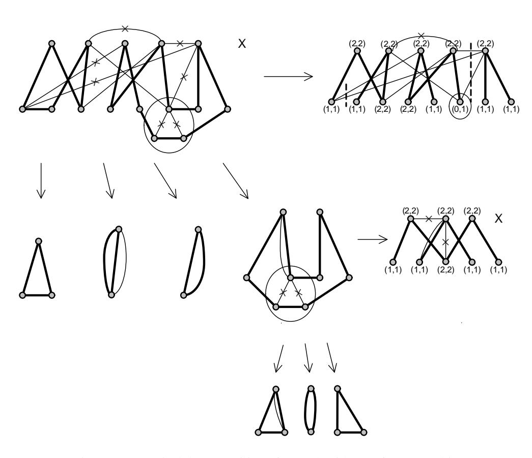
Figure 2. Canonical decomposition of a graph with a perfect 2-matching

This theorem describes a way to decompose general graphs with degree-matchings into matching covered subgraphs. It is instructive to study the example shown in Figure 2, which demonstrates how the decomposition by means of extreme set works (the critical subgraphs are circled).

We have proved a result generalizing the Gallai-Edmonds Structure Theorem. Just as in the case of perfect matchings, this theorem has many consequences and applications. In this work we do not treat any of these, but some of them are discussed in [2].

5. Graphs with perfect (g, f)-matchings

In this section we focus on the problem for the more general version of degree-factors. Similarly, we could define that a set of vertices X in V (G) is extreme with respect to (g, f)-matchings if the following inequalities hold

\[\delta(G) + g(X) \le \delta(G - X) \le \delta(G) + f(X).\]

Observe that this formula is general and, for g ≡ f, it is equivalent to the one for f-matchings, and for g ≡ f ≡ 1 it is the same as for ordinary matchings. However, although our definition is analogous to that of an extreme set with respect to f-matchings, we will see that the extreme sets with respect to (g, f)-matchings have slightly different properties.

The following properties can be determined. The situation here is much more complicated given the lack of the systematic theory, as the following examples illustrate. Consider the graph in Figure 3 (on the left). According to our definition, this graph has the extreme sets ∅ (trivial), {2}, {3}, {1, 2}, {1, 3} and {2, 3}, but singletons {1}, {4} or {5} are not extreme. The maximal extreme set is {1, 2, 3} and there are no other extreme sets.

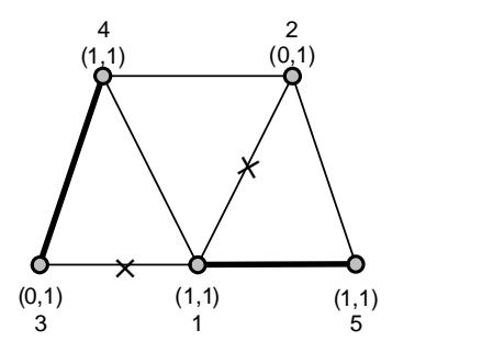
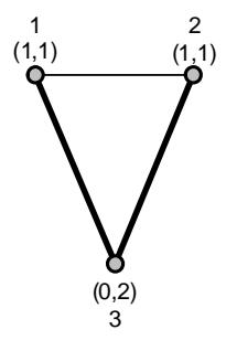
Figure 3. Elementary graphs with perfect (g, f)-matchings

Consider now the graph on the right. The singleton {3} is extreme, but neither {1} nor {2} is extreme. The maximal (non-trivial) extreme sets are {1, 3}, and {2, 3}, there are no other extreme sets and no other proper subset of these extreme sets is extreme. Note that although edges {1, 3} and {2, 3} are allowed, they join two vertices belonging to a (maximal) extreme set.

Further, observe that there exists no (g, f)-factor F with d^F (3) = 1. Thus, an interesting question is whether we can determine vertices in a general graph whose degrees are not consecutive in (g, f)-matchings. According to Theorem 2.3 these can be only vertices that belong to the set C(G) of the Lovasz-Plummer Canonical Decomposition.

We have seen that the situation is considerably more complex for (g, f)-matchings. In fact, most of the properties of extreme sets do not hold. An alternative way to find the decomposition of edges is based on a reduction to the f-matching problem.

6. Conclusion

In this paper, the extreme sets have been defined for f-matchings. We have an open problem that could not be solved in this paper: can an extreme set be defined for an arbitrary perfect (g, f) matching without transformation to a perfect f-matching?

Finally, we point out that in the present paper we consider only structural properties of extreme sets. However, there are interesting complexity issues concerning the detection and handling of extreme sets, which can be the subject of the future work.

References

• [1] A. Busch, M. Ferrara, and N. Kahl, Generalizing D-graphs, Discrete Applied Mathematics 155 (18) (2007), 2487–2495.
• [2] R. Cymer, Gallai-Edmonds decomposition as a pruning technique, Central European Journal of Operations Research 23 (1) (2015), 149–185.
• [3] P. Fraisse, P. Hell and D.G. Kirkpatrick, A note on f-factors in directed and undirected multigraphs, Graphs and Combinatorics 2 (1) (1986), 61–66.
• [4] P. Katerinis, Some results on the existence of 2n-factors in terms of vertex-deleted subgraphs, Ars Combinatoria 16B (1983), 271–277.
• [5] N. Kita, A partially ordered structure and a generalization of the canonical partition for general graphs with perfect matchings, Lecture Notes in Computer Science 7676 (2012), 85–94. Springer.
• [6] A. Kotzig, On the theory of finite graphs with a linear factor I, Matematicko-Fyzikalny ´ Casopis Slovenskej Akad ˇ emie Vied ´ 9 (2) (1959), 73–91. In Slovak.
• [7] A. Kotzig, On the theory of finite graphs with a linear factor II, Matematicko-Fyzikalny ´ Casopis Slovenskej Akad ˇ emie Vied ´ 9 (2) (1959), 136–159. In Slovak.
• [8] A. Kotzig, On the theory of finite graphs with a linear factor III, Matematicko-Fyzikalny ´ Casopis Slovenskej Akad ˇ emie Vied ´ 10 (4) (1960), 205–215. In Slovak.
• [9] L. Lovasz, On the structure of factorizable graphs, ´ Acta Mathematica Academiae Scientiarum Hungaricae 23 (1972), 179–195.
• [10] L. Lovasz, On the structure of factorizable graphs. II, ´ Acta Mathematica Academiae Scientiarum Hungaricae 23 (1972), 465–478.

A note on extreme sets | Radosław Cymer

• [11] L. Lovasz and M. D. Plummer, Matching theory, ´ Annals of Discrete Mathematics 29 (1986), North-Holland, Amsterdam.
• [12] S. Wang and J. Hao, The extreme set condition of a graph, Discrete Mathematics 260 (1-3) (2003), 151–161.