V. Yegnanarayanan
Department of Mathematics School of Humanities and Sciences SASTRA University Thanjavur-613401, Tamilnadu, India
prof.yegna@gmail.com
Let p ≥ 3 be a positive integer and let k ∈ {1, 2, . . . p − 1}\bp/2c. The generalized Petersen graph GP((p, k) has its vertex and edge set as V (GP(p, k)) = {ui : i ∈ Zp} ∪ {u 0 i : i ∈ Zp} and E(GP(p, k)) = {uiui+1 : i ∈ Zp} ∪ {u 0 iu 0 i+k ∈ Zp} ∪ {uiu 0 i : i ∈ Zp}. In this paper we probe its spectrum and determine the Estrada index, Laplacian Estrada index, signless Laplacian Estrada index, normalized Laplacian Estrada index, and energy of a graph. While obtaining some interesting results, we also provide relevant background and problems.
Keywords: generalized Petersen graph, spectrum, Estrada index, Laplacian Estrada index, normalized Estrada index, signless Laplacian Estrada index, energy of a graph.
Mathematics Subject Classification : 05C07, 05C12, 05C42, 05C50,05C75.
DOI:10.5614/ejgta.2017.5.2.1
1. Introduction
The graphs considered in this paper are all finite, simple and undirected.
In parallel computing and computer networks, several different topologies for interconnecting processing vertices exist. It is quite an enormous task to compare such networks with reference to attributes such as diameter, average distance, traffic balance, fault tolerance etc. In order to overcome the inherent drawbacks in ring topology, it is suggested to have a P-vertex ring that
Received: 12 December 2016, Revised: 19 May 2017, Accepted: 19 June 2017.
could lead to a double ring network. These notions have led to the generalized Petersen graph. Let p ≥ 3 be a positive integer and let k ∈ {1, 2, . . . p − 1}\p/2. The generalized Petersen graph GP((p, k) has its vertex and edge set as V (GP(p, k)) = {ui : i ∈ Zp} ∪ {u 0 i : i ∈ Zp} and E(GP(p, k)) = {uiui+1 : i ∈ Zp} ∪ {u 0 iu 0 i+k ∈ Zp} ∪ {uiu 0 i : i ∈ Zp}. They form a pertinent family of 4-connected, 3-regular graphs with 2p vertices and 3p edges. These graphs are generally used in interconnection networks. The Petersen graph is definitely a sought after objects among the graph theory community. It has served as a counter example to several open problems and conjectures. Even though it is cubic and without cut edges is not 1-factorizable and nonhamiltonian. Another surprising aspect is that it is highly symmetric even though its automorphism graph on directed paths of length three is transitive. Here we probe its spectrum and determine the Estrada index, Laplacian Estrada index, Signless Laplacian Estrada index, normalized Laplacian Estrada index, and energy of a graph. While obtaining some interesting results, we also provide relevant background and problems.
1.1. Graph spectra
Graph spectra's presence is quite eminent in internet, artificial intelligence and other related areas. The largest eigen value plays a vital role to mathematically describe spreading of virus in computer network. For an exhaustive review on graph spectra and its applications one can refer to [29]. A seminal mathematical paper that deals with graph spectra [20] is outcome of an attempt to solve approximately a partial differential equation which models a membrane vibration problem. Among the research community in general and members of mathematics community in particular who bothers graphs and its properties seriously are largely attracted by the distinct eigen values of a graph which are very small in number. It is well known that graphs with lesser number of distinct eigen values are highly symmetric and mostly possess small diameter. This is one of the main reasons that motivated us to write this paper on the generalized Petersen graph. It is still open problem to completely characterize classes of regular graphs with given number 'k' of distinct eigen values where k is a positive integer which is very small. Also for interesting mathematical properties regarding the largest value, smallest and second smallest eigen values one can refer to [29].
1.2. Estrada index
Estrada index was coined to represent the inherent features of organic modules in its 3-D structure. Ernesto Estrada, a Cuban-Spanish mathematician coined in the year 2000, a new descriptor called the Estrada index, denoted by EE [14]. Originally it was meant to quantify long chain molecule's degree of folding. The EE values of constructed weighted graphs play a crucial role in the protein molecules. Infact it is a measure of complex network's centrality. For more on the variety of applications one can see [3]. A simple graph G with p vertices and q edges are called normally as a (p − q) graph. By the eigen values of G we mean the eigen values of the adjacency matrix A(G) of G. We denote them by λ1 ≥ λ2 ≥ · · · ≥ λp. The whole set of eigen values values of G form the spectrum of G. The Estrada index, EE(G) = X p i=1 e λi where λi are the eigen values of G. In [23, 25, 26] the author has found new lower bounds for the Estrada index, Estrada index for Ramanujan graphs and perturbation results for Estrada index of weighted networks.
1.3. Laplacian Estrada index
As an interesting extension to Estrada index the authors in [4] have introduced the notion of Laplacian Estrada index of a Graph. A number of interesting results about LEE were found in [4, 30] and for additional latest results one can refer to [18] and the reference therein. The Laplacian matrix of G is L(G) = D(G)−A(G) where D(G) = diag[d1, d2, . . . , dp] is the diagonal matrix of vertex degrees of G. We denote the eigen values of D(G) by µi , i = 1 to p. The Laplacian p
Estrada index is LEE(G) = X i=1 e µi . The matrix L +(G) = D(G)+A(G) is referred as the signless Laplacian matrix of G and its eigen values are denoted by ηi , i = 1 to p.
1.4. Signless Laplacian Estrada index
The authors in [1] have coined a new index in the mould of Estrada index namely signless Laplacian Estrada index (SLEE). Although LEE and SLEE merge with each other when restricted to the family of bi-partite graphs, SLEE offers noteworthy variations when we consider fullerenes and other non-alternant conjugated species [1]. The matrix L +(G) = D(G) + A(G) is referred as the signless Laplacian matrix of G and its eigen values are denoted by η1, η2, . . . , ηp. The signless
Laplacian Estrada index is SLEE(G) = X p i=1 e ηi . The study of the spectral properties of the matrix L +(G) has started only very recently.
1.5. Normalized Estrada index
The authors in [15] have introduced another variation to Estrada index namely normalized Laplacian Estrada index. For fundamental properties of `EE one can also see [19], The normalized Laplacian matrix `(G) = (`ij )p×p where `ij = 1 if i = j and deg(vi) 6= 0; (−1)/(d(vi)d(vj ))1/2 if i 6= j and vi is adjacent to vj ; 0 otherwise. Normalized Laplacian eigen values G are denoted by 0 ≤ δ1 ≤ δ2 ≤ · · · ≤ δp. The normalized Estrada index is `EE(G) = X p i=1 e δi .
The author in [24] studied the logarithm of the Estrada index as a spectral measure to characterize the robustness of complex networks. He derived novel analytic lower bounds for the logarithm of the Estrada index based on the Laplacian spectrum and the mixing times of random walks on the network. The main techniques he employed are some inequalities, such as the thermodynamic inequality in statistical mechanics, a trace inequality of von Neumann, and a refined harmonicarithmetic mean inequality.
The idea of computing SLEE, LEE and EE of a well-known family like the generalized Petersen graph is to explore the possibility of making them serve as a mathematical model for chemically non-alternant conjugated species. It is a well known that graphs with lesser number of distinct eigen values are highly symmetric and mostly possess small diameter. This is one of the main reasons that motivated us to look at the generalized Petersen graph. Also see [4, 30, 18, 1, 15, 19, 6, 7].
1.6. Energy and its variations
The concept of energy arose in chemistry. Molecular orbital theory due to Hückel is a subfield of theoretical chemistry wherein the graph eigenvalues occur. The carbon atoms of a hydrocarbon system are represented as vertices of a graph associated with the molecule. From Hückel theory, the energy of a molecular graph is equal to the total \(\pi\)-electron energy of a conjugated hydrocarbon.
Even though the concept of graph energy is not considered as significant among the mathematical community when it was proposed. Later it has steadily attracted the attention and a number of research papers started pouring out from the minds of mathematicians. To know more about this one can refer to [10, 11, 2, 8]. The 3-regular generalized Petersen graph obeys this property. In-fact there are only five graphs known as on data with E(G) assuming values less than the number of vertices of G. The energy E(G) is defined as the sum of absolute values of the eigen values [16, 5].
In [9, 12, 13, 17, 28] the authors have categorized graphs on p-vertices and obeys E(G) > 2p-2 as hypo-energetic and those violate this as energy non-hypo energetic. To comprehend the logic behind defining hyperenergeticity one needs to observe the following. In those periods when computers were not available, to calculate HMO total \(\pi\)-energy (that is, E) much effort was made to find simple algebraic expressions to obtain an approximate numerical value of E perusing the simple structural details of the underlying molecular graph. One such approximation was due to McClelland [21] viz. \(E \approx a\sqrt{2pq}\) where p and q are the number of vertices also denotes number of carbon atoms and number of edges also stands for number of carbon-carbon bonds of the corresponding molecular graph and where a is an empirical constant \(a \approx 0.9\). Alternately one can also call a graph with p vertices to be hypo-energetic if E(G) < p. Normalized Laplacian
energy of the graph \[G\] is defined as \(E_{\ell}(G) = \sum_{i=1}^{p} |\delta_i - 1|\).
Note that if a graph is non-singular then it is non-hypo energetic. This is because \((1/p)E(G) \ge (\prod_{i=1}^p |\lambda_i|^{1/p}) = |\det(A(G))|^{1/p}\). As \(|\det(A(G))| \ge 1\) (here \(\det(A(G))\) stands for the determinant of A(G)) this implies \(|\det(A(G))|^{1/p} \ge 1\). But the converse is not true. That is if G is non-hypo energetic then it is not necessary that it should be non-singular. For instance the graph GP(3,1)
is non hypo energetic as \[E(GP(3,1)) = \sum_{i=1}^{6} |\lambda_i| = 7.236 > |V(GP(3,1))| = 6\]. But two
of its eigen values equal to zero. Is GP(3t,1) singular and non-hypo energetic for all \(t\geq 1\)? In [29] it has been established that for any graph with p vertices and q edges if \(q\geq p^2/4\) then G is non-hypo energetic. But the converse need not be true. For instance, consider the graph GP(4,1). Note that |V(GP(4,1))|=8 and |E(GP(4,1))|=12. Note that \(12\geq 8^2/4=16\). Similarly the other generalized Petersen graphs serving as likewise examples are GP(5,1), GP(6,1), GP(7,1) etc. This induces us to conclude that GP(p,1) is non-hypo energetic but \(|E(GP(p,1))|\geq |V(GP(p,1)|^2/4\) for \(p\geq 4\). Moreover the fact \(3p\geq (2p)^2/4\) is possible if and only if \(p\leq 3\). Hence GP(3,1) is the only graph among the class of generalized Petersen graph to posses the property of being non-hypo energetic with \(|E(GP(p,1))|\geq |V(GP(p,1)|^2/4\).
1.7. Chromatic number of a graph
By the chromatic number of a graph G we mean the least number of colors used to properly color the vertices of G such that no two adjacent vertices are colored same. This coloring parameter
is denoted by \(\chi(G)\). The chromatic number of the generalized Petersen graph is computed for academic interest for a few special cases to indicate how the vertex of it is split into two or three sets depending on the fact that they are bipartite or not. Also there is an interesting relationship between chromatic number and the first largest eigen value of the adjacency matrix of a graph and the same is exploited in the proof of Theorem 2.5.
2. Main results
Proposition 2.1. GP(2r, 2s + 1) is bi-partite.
Corollary 2.1. \(\chi(GP(2r,\ell)) = 2\) for any odd '\(\ell\)'.
Proposition 2.2. \(\chi(GP(2r, 2k)) = 3\) for any r, k.
Theorem 2.1. \(2\sqrt{p^2+3p} \le EE(GP[p,k]) \le (2p-1) + e^{\sqrt{6p}}\).
Theorem 2.2. \(LEE(GP(p,k)) \ge 1 + e^4 + 2(p-1)e^{\left(\frac{3p-2}{p-1}\right)}\).
Theorem 2.3. \(LEE(GP(p,k)) \le exp\{3\{2p-1-LE(GP[p,k])\}\} + exp\{LE(GP[p,k])\}\)
where LE(G) indicates Laplacian energy of G defined by \(LE(G) = \sum_{i=1}^{p} \left| \mu_i - \frac{2q}{p} \right|\).
Theorem 2.4. \(LEE(G^*) \leq 8p - 1 - 2\sqrt{6p} + e^{2\sqrt{6p}}\).
Theorem 2.5. \(SLEE(Gp(2r,1)) \ge e^2 + (p-1)e^{\left(-\frac{2-2q}{p-1}\right)}\).
Corollary 2.2. \(SLEE(Gp(2r+1,k)) \ge e^4 + (p-1)e^{\left(-\frac{4-2q}{p-1}\right)}\) for any k.
Theorem 2.6. Let G[p,k] be any generalized Petersen graph with \(k \leq \lfloor \frac{p-1}{2} \rfloor\). Then \(\ell EE(GP[p,k]) \geq 1 + (p-1)^{\frac{p}{p-1}}\).
Theorem 2.7. \(2\sqrt{p^2+3p} \le EE(GP[p,k]) \le (2p-1) + e^{\sqrt{6p}}\).
3. Proofs of main results
Proof of Proposition 2.1:
For s=0, it is obvious. We give construction for P(2r,2t+1). Let \((V_1,V_2)\) be the bi-partition of the vertex set of GP(2r,2t+1) with \(V_1=\{u_{2j-1},v_{2i}:1\leq j\leq r,1\leq i\leq r\}\) and \(V_2=\{u_{2i},v_{2j-1}:1\leq i\leq r,1\leq j\leq r\}\). The edge set of GP(2r,2t+1) is \(E[GP[2r,2t+1]]=\{(u_{2j-1},u_{2j}),1\leq j\leq r;(u_i,v_i),0\leq i\leq 2r;(u_0,u_1);(v_i,v_{i+t(mod\ 2r)}),0\leq i\leq 2r-1\}\). Then for the graph GP(2r,2t+3) just keep the vertex set bi-partition exactly as in GP(2r,2t+1) and construct the edge set in a similar manner. Like this one can modify the edge set of GP(2r,k) for any odd k by retaining the vertex bi-partite sets.
Proof of Proposition 2.2:
Let \(V(GP(2r,2k))=\{u_iu_i':1\leq i\leq 2p\}\) and \(E(GP(2r,2k))=\{u_iu_i':1\leq i\leq 2r,u_iu_{i+1}:1\leq i\leq 2r-1,u_{2r}u_1,u_i'u_{2k+i(mod\ 2r)}:1\leq i\leq 2r\}\). Note that \(C_{2k+3}\) is an induced subgraph of GP(2r,2k). As \(\chi\) is a monotone function and the chromatic number of an odd cycle is 3, we have \(3=\chi(c_{2k+3})\leq \chi(GP(2r,2k))\). We now exhibit a chromatic 3-coloring of GP(2r,2k) to complete the proof. Let \(f:V(GP(2r,2k))\to\{c_1,c_2,c_3\}\) be a function such that \(f(v_i)=c_i\) for \(1\leq i\leq s\) where \(V_1=\{u_i:i\equiv 0(mod\ 3),u_i':i\equiv 1(mod\ 3)\}\), \(V_2=\{u_i:i\equiv 1(mod\ 3),u_i':i\equiv 2(mod\ 3)\}\), \(V_3=\{u_i:i\equiv 2(mod\ 3),u_i':i\equiv 0(mod\ 3)\}\). Then one can check that \((V_1,V_2,V_3)\) constitutes a partition of the vertex set GP(2r,2k).
Proof of Theorem 2.1:
Let \[G^*=GP[p,k]\]. Then from \(EE=EE(G)=\sum_{i=1}^{2p}e^{\lambda_i}\) We get \(EE^2=2p\sum_{i=1}e^{2\lambda_i}+2\sum_{i=1}^{2p}\sum_{i=1}e^{\lambda_i}\) with the help of the inequality between arithmetic mean and geometric mean, we infer that \(2\sum_{i< j}\sum e^{\lambda_i\lambda_j}\geq 2p(2p-1)\left(\prod_{i< j}e^{\lambda_i\lambda_j}\right)^{\frac{2}{2p(2p-1)}}=2p(2p-1)\left[\left(\prod_{i=1}^{2p}e^{\lambda_i}\right)^{2p-1}\right]^{\frac{2}{2p(2p-1)}}\) \(=2p(2p-1)\left[(mxp(\sum_{i=1}^{2p}\lambda_i))^{\frac{1}{p}}=2p(2p-1)\right]\). Further, \(2p\sum_{i=1}^{2p}e^{2\lambda_i}=\sum_{i=0}\sum_{k\geq 0}\frac{(2\lambda_i)^k}{k!}=2p+1\) \(12p+\sum_{i=1}^{2p}\sum_{k\geq 3}\frac{(2\lambda_i)^k}{k!}\). As \(\sum_{i=1}^{2p}\sum_{k\geq 3}\frac{(2\lambda_i)^k}{k!}\geq 8\sum_{i=1}^{2p}\sum_{k\geq 3}\frac{(\lambda_i)^k}{k!}\), we can choose a constant \(\beta\in[0.8]\) so that \(2p\sum_{i=1}^{2p}e^{2\lambda_i}\geq 2+12p+\beta\sum_{i=1}^{2p}\sum_{k\geq 3}\frac{(\lambda_i)^k}{k!}=2p+12p-2\beta p-3\beta p+\beta\sum_{i=1}^{2p}\sum_{k\geq 3}\frac{(\lambda_i)^k}{k!}\). So \(\sum_{i=1}^{2p}e^{2\lambda_i}\geq 2(1-\beta)p+3(4-\beta)p+\beta EE\). A little elementary computations show that \(EE\geq\frac{\beta}{2}+\sqrt{\left(2p-\frac{\beta}{2}\right)^2+3(4-\beta)p}\). Now observe that for \(p\geq 1\) the function \(\frac{\beta}{2}+\sqrt{\left(2p-\frac{\beta}{2}\right)^2+3(4-\beta)p}\) decreases. A lower bound for \(EE\) occurs at \(\beta=0\). That is, \(EE(G^*)\geq 2\sqrt{p^2+3p}\). (While deriving this we made use of the fact that \(\sum_{i=1}^{2p}\frac{(2\lambda_i)^0}{0!}=2p\), \(\sum_{i=1}^{2p}\sum_{k\geq 1}\frac{(\lambda_i)^k}{k!}\leq 2p+\sum_{i=1}^{2p}\sum_{k\geq 1}\frac{|\lambda_i|^k}{k!}=2p+1\)
On some aspects of the generalized Petersen graph V. Yegnanarayanan
\[\sum_{k \geq 1} \frac{1}{k!} \sum_{i=1}^{2p} [(\lambda_i)^2]^{\frac{k}{2}} \leq 2p + \sum_{k \geq 1} \frac{1}{k!} \left[ \sum_{i=1}^{2p} (\lambda_i)^2 \right]^{\frac{k}{2}} = 2p + \sum_{k \geq 1} \frac{1}{2!} (6p)^{\frac{k}{2}} = 2p - 1 + \sum_{k \geq 0} \frac{(\sqrt{6p})^k}{k!} \text{ which in turns gives the required upper bound.}\]
Proof of Theorem 2.2:
As GP(p,k) is connected, \(\mu_{2p}=0\). Therefore \(LEE\{GP(p,k)\}=1+\sum_{i=1}^{2p-1}e^{\mu_i}\geq 1+e^{\mu_i}+(2p-2)e^{(\mu_1+\mu_2+\cdots\mu_{2p-1})/2p-2)}=1+e^{\mu_i}+(2p-2)e^{6p-2/2p-2}\). This is because of the application of arithmetic-geometric mean inequality and that \(\mu_1+\mu_2+\cdots+\mu_{2p-1}=6p\). If \(g(\theta)=e^{\theta}+(2p-2)e^{\left\{\frac{6p-\theta}{2p-2}\right\}}\) then \(g'(\theta)=e^{\theta}-e^{\left\{\frac{6p-\theta}{2p-2}\right\}}\). Hence g is an increasing function for \(\theta\geq\frac{6p}{2p-1}\). Next note that \(\frac{6p}{2p-1}\leq 4\). Also \(\mu_1\geq 4\) [7]. Hence from \(g(\mu_1)\geq g(4)\) the result follows.
Proof of Theorem 2.3:
First observe that \[\sum_{i=1}^{p} (\mu_i - 3) = 0\] and \(\mu_i \ge 3\). Now \(e^{-3}LEE(GP[p,k]) = \sum_{i=1}^{2p} e^{(\mu_i - 3)} = 2p + \sum_{k\ge 2} \frac{1}{k!} \sum_{i=1}^{2p} |\mu_i - 3|^{k_0} \le 2p + \sum_{k\ge 2} \frac{1}{k!} \left(\sum_{i=1}^{2p} |\mu_i - 3|^{k_0}\right) = 2p + \sum_{k\ge 2} \frac{1}{k!} LE(GP[p,k])^{k_0} = 2p - 1 - LE(GP(p,k)) + exp\{LE(GP(p,k))\}.\)
Proof of Theorem 2.4:
First note that \[\sum_{i=1}^{2p} \mu_i^2 = 18p + 2(3p) = 24p\]. So for \(k \in Z^+\) with \(k \ge 3\), we have \(\left(\sum_{i=1}^{2p} \mu_i^2\right)^k \ge \sum_{i=1}^{2p} \mu_i^{2k} + k \sum_{1 \le i < j \le 2p} [\mu_i^2 \mu_j^{2(k-1)} + \mu_i^{2(k-1)} \mu_j^2] \ge \sum_{i=1}^{2p} \mu_i^{2k} + 2k \sum_{1 \le i < j \le 2p} \mu_i^k \mu_j^k \ge \left(\sum_{i=1}^{2p} \mu_i^k\right)^2\). Hence \(\sum_{i=1}^{2p} \mu_i^k \le \left(\sum_{i=1}^{2p} \mu_i^2\right)^{\frac{k}{2}} = (24p)^{\frac{k}{2}}\). Now \(LEE(G^*) = 2p + 6p + \sum_{k \ge 2} \frac{1}{k!} \sum_{i=1}^{2p} \mu_i^k \le 2p + 6p + \sum_{k \ge 2} \frac{1}{k!} (24p)^k = 8p - 1 - 2\sqrt{6p} + e^{2\sqrt{6p}}\).
Proof of Theorem 2.5:
As GP[2r,1] is a connected graph, \(\eta_1 \geq 0\). By using the arithmetic-geometric mean inequality (as in Theorem 2.1) we derive that \(SLEE(GP[2r,1]) = e^{\eta_1} + e^{\eta_2} + \cdots + e^{\eta_p} \geq e^{\eta_1} + (p-1)(\sum_{i=1}^p e^{\eta_i})^{1/p-1}\).
Now as \(\sum_{i=1}^p \eta_i = 2q\) we have \(SLEE(GP[2r,1]) \geq e^{\eta_1} + (p-1)\left[e^{2q-\eta_1}\right]^{\frac{1}{p-1}}\) (*). Consider the function \(g(x) = e^x + (p-1)e^{-\left(\frac{x-2q}{p-1}\right)}\). Clearly g'(x) > 0 if x > 0. We know that for any simple graph, with chromatic number \(\chi\), \(\lambda_1 \geq \chi - 1\) (**) Therefore the result follows with the help of (*) and (**).
Proof of Corollary 2.2:
It follows from the Theorem 2.5 and the fact that \(\chi[(GP[2r+1,k])=3.\)
Proof of Theorem 2.6:
It is easy to check that \(\delta_1 = 0\) for any GP(p, k). So \(\sum_{i=2}^p \delta_i = p\), the number of vertices and hence
\[\ell EE(Gp[p,k)] = 1 + \sum_{i=2}^{p} e^{\delta_i} \geq 1 + (p-1)e^{\frac{\left(\sum_{i=2}^{p} \delta_i\right)}{p-1}} = 1 + (p-1)e^{\frac{p}{p-1}} \text{ (by AM-GM-mean inequality)}.\]
Proof of Theorem 2.7:
Let \[G^*=GP[p,k]\]. Then from \(EE(G)=\sum_{i=1}^{2p}e^{\lambda_1}\) We get \(EE^2=\sum_{i=1}^{2p}e^{2\lambda_i}+\sum\sum\sum_{i=1}e^{\lambda_i}e^{\lambda_i}\) where \(i< j\). With the help of the inequality between arithmetic mean and geometric mean, we infer that \(2\sum_{i< j}\sum e^{\lambda_i\lambda_j}\geq 2p(2p-1)\left(\prod_{i< j}e^{\lambda_i}e^{\lambda_j}\right)^{\frac{2}{2p(2p-1)}}=2p(2p-1)((\prod_{i=1}^{2p}e^{\lambda_i})^{\frac{2}{2p-1}})^{\frac{2}{2p(2p-1)}}=2p(2p-1)(\exp(\sum_{i=1}^{2p}\lambda_i))^{\frac{1}{p}}=2p(2p-1).\) Further \(\sum_{i=1}^{2p}e^{2\lambda_i}=\sum_{i=0}^{2p}\sum_{k\geq 0}\frac{(2\lambda_i)^k}{k!}=2p+12p+12p+12p+12p+12p+12p+12p+12p+12p+1\)
decreases in [0,8]. Hence the tight lower bound for EE occurs at \(\beta=0\). That is, \(EE(G^*)\geq 2\sqrt{p^2+2p}\). While deriving this we made use of the fact that \(\sum_{i=1}^{2p}\frac{(2\lambda_i)^0}{0!}=2p\) and \(\sum_{i=1}^{2p}\frac{(2\lambda_i)^1}{1!}=0\) and \(\sum_{i=1}^{2p}\frac{(2\lambda_i)^2}{2!}=4(3p)\). To achieve the upper bound note that \(EE=2p+\sum_{i=1}^{2p}\sum_{k\geq 1}\frac{(\lambda_i)^k}{k!}\leq 2p+\sum_{i=1}^{2p}\sum_{k\geq 1}\frac{|\lambda_i|^k}{k!}=2p+\sum_{k\geq 1}\frac{1}{k!}\sum_{i=1}^{2p}[(\lambda_i)^2]^{\frac{k}{2}}\leq 2p+\sum_{k\geq 1}\frac{1}{k!}\left[\sum_{i=1}^{2p}(\lambda_i)^2\right]^{\frac{k}{2}}=2p+\sum_{k\geq 1}\frac{1}{2!}(6p)^{\frac{k}{2}}=2p-1+\sum_{k\geq 0}\frac{(\sqrt{6p})^k}{k!}\) which in turns gives the required upper bound.
4. Numerical computation of various Estrada indices for GP(p, k) for some p and k
Using Mat lab we have calculated EE(GP(p,k)), LEE(GP(p,k)), SLEE(GP(p,k)) and \(\ell EE(GP(p,k))\) for p=3 to 8 and k=1 to 3. Different generalized Petersen graphs and their respective Estrada indices are given below:
Figure 1: GP(3,1) EE = 24.2544 LEE = 301.7051 \(\ell EE = 18.6048\)SLEE = 487.565
\(\begin{aligned} & \text{Figure 2: } GP(4,1) \\ & EE = 29.3939 \\ & LEE = 590.3907 \\ & SLEE = 590.3907 \\ & \ell EE = 25.6130 \end{aligned}\)
Figure 3: GP(5, 1) EE = 33.2993 LEE = 684.7497 SLEE = 712.6166\(\ell EE = 31.6940\)
Figure 4: GP(5, 2) EE = 34.2182 LEE = 631.5983 SLEE = 687.293 IEE = 31.9178
Figure 5: GP(6, 1) EE = 42.2703 LEE = 856.4102 SLEE = 849.0211 IEE = 32.9473
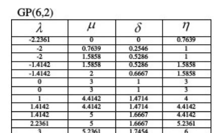
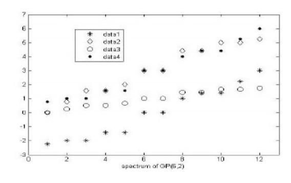
Figure 6: GP(6, 2) EE = 43.2507 LEE = 710.4666 SLEE = 868.7108 IEE = 38.0957
Figure 7: GP(7, 1) EE = 49.2564 LEE = 988.9037 SLEE = 989.331 IEE = 44.7814
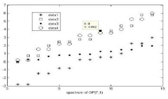
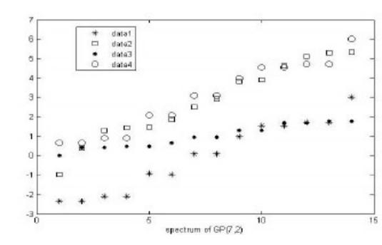
Figure 8: GP(7, 2) EE = 46.6754 LEE = 820.1843 SLEE = 937.505 IEE = 44.692
Figure 9: GP(8, 1) EE = 56.3009 LEE = 1130.4687 SLEE = 1075.8705 IEE = 51.1781
Figure 10: GP(8, 2) EE = 44.7758 LEE = 1048.6051 SLEE = 898.9929 IEE = 51.0998
Figure 11: GP(8, 3) EE = 52.7103 LEE = 1058.7175 SLEE = 1070.9476 IEE = 51.0857
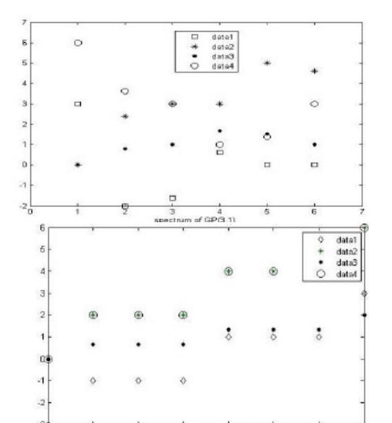
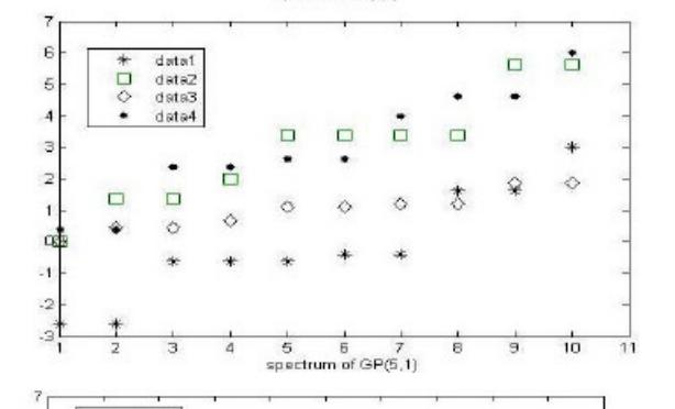
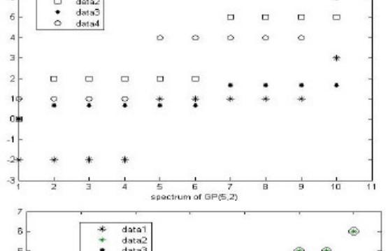
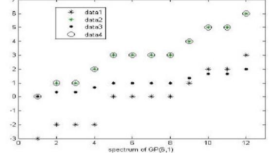
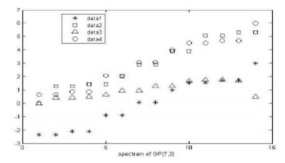
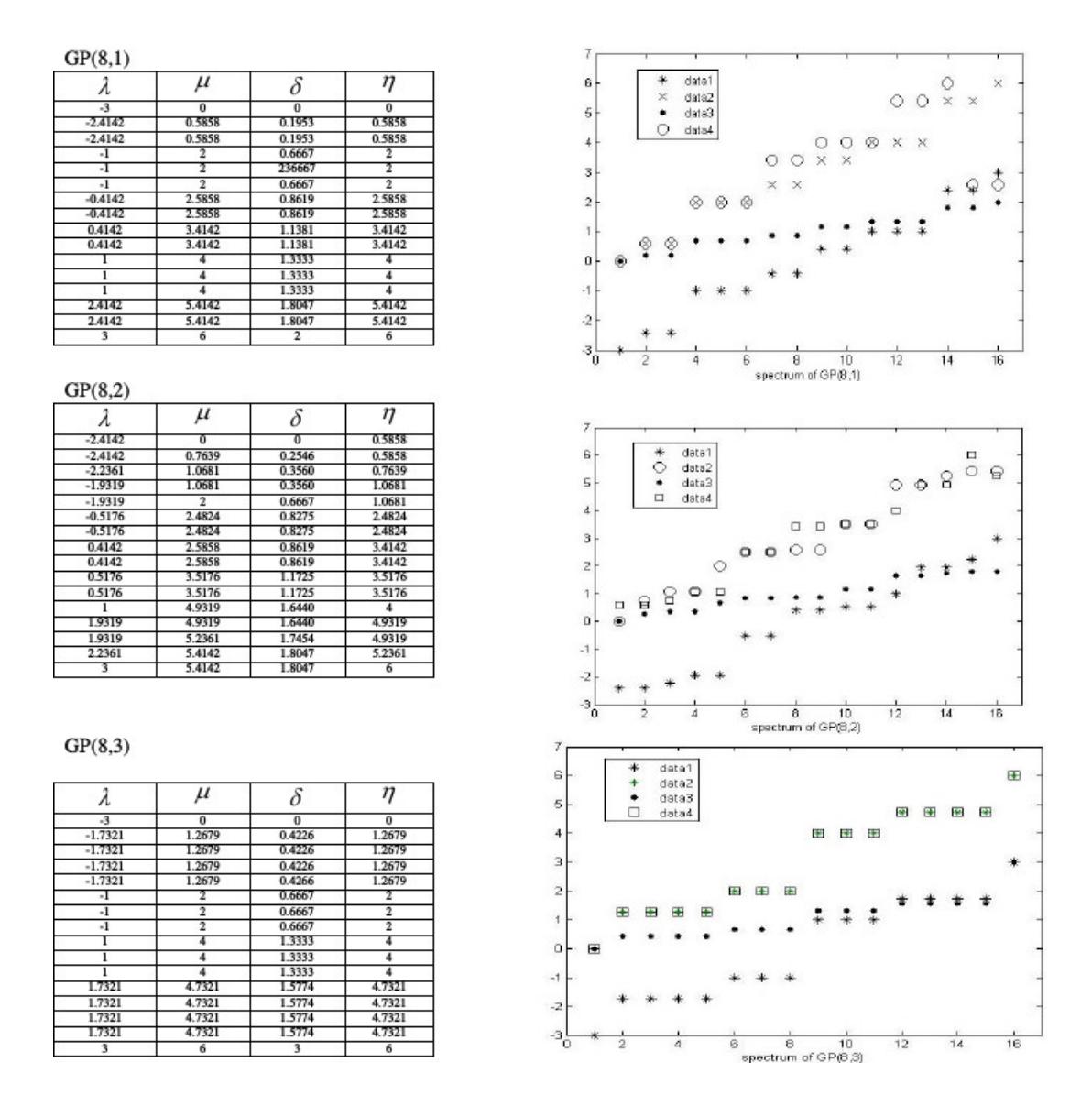
Using Mat Lab we have plotted the spectrum of GP(p, k) obtained for various and respective underlying matrices. we denote various spectrum as follows:
On some aspects of the generalized Petersen graph | V. Yegnanarayanan
| λ | μ | δ | η |
|---|---|---|---|
| -2 | 0 | 0 | 1 |
| -1.6180 | 2.3820 | 0.7940 | 1.3820 |
| 0 | 3 | 1 | 3 |
| 0 | 3 | 1 | 3 |
| 0.6180 | 4.6180 | 1.5393 | 3.6180 |
| 3 | 5 | 1.6667 | 6 |
| λ | μ | δ | η |
|---|---|---|---|
| -3 | 0 | 0 | 0 |
| -1 | 2 | 0.6667 | 2 |
| -1 | 2 | 0.6667 | 2 |
| -1 | 2 | 0.6667 | 2 |
| 1 | 4 | 1.3333 | 4 |
| 1 | 4 | 1.3333 | - 4 |
| 1 | 4 | 1.3333 | 4 |
| 3 | 6 | 2 | 6 |
| λ | μ | δ | η |
|---|---|---|---|
| -2.6180 | 0 | 0 | 0.3820 |
| -2.6180 | 1.3820 | 0.4607 | 0.3820 |
| -0.6180 | 1.3820 | 0.4607 | 2.3820 |
| -0.6180 | 2 | 0.6667 | 2.3820 |
| -0.6180 | 3.3820 | 1.1273 | 2.6180 |
| -0.3820 | 3.3820 | 1.1273 | 2.6180 |
| -0.3820 | 3.3820 | 1.2060 | 4 |
| 1.6180 | 3.3820 | 1.2060 | 4.6180 |
| 1.6180 | 5.6180 | 1.8727 | 4.6180 |
| 3 | 5.6180 | 1.8727 | 6 |
| λ | μ | δ | η |
|---|---|---|---|
| -2 | 0 | 0 | 1 |
| -2 | 2 | 0.6667 | - 1 |
| -2 | 2 | 0.6667 | 1 |
| -2 | 2 | 0.6667 | 1 |
| 1 | 2 | 0.6667 | 4 |
| 1 | 2 | 0.6667 | 4 |
| 1 | 5 | 1.6667 | 4 |
| 1 | 5 | 1.6667 | 4 |
| 1 | 5 | 1.6667 | 4 |
| 3 | 5 | 1.6667 | 6 |
| λ | μ | δ | η |
|---|---|---|---|
| -3 | 0 | 0 | 0 |
| -2 | 1 | 0.3333 | - 1 |
| -2 | 1 | 0.3333 | - 1 |
| -1 | 2 | 0.6667 | 2 |
| 0 | 3 | 1 | 3 |
| 0 | 3 | 1 | 3 |
| 0 | 3 | 1 | 3 |
| 0 | 3 | 1 | 3 |
| 1 | 4 | 1.3333 | 4 |
| 2 | 5 | 1.6667 | 5 |
| 2 | 5 | 1.6667 | 5 |
| 3 | 6 | 2 | 6 |
On some aspects of the generalized Petersen graph | V. Yegnanarayanan
| λ | μ | δ | η |
|---|---|---|---|
| -2.8019 | 0 | 0 | 0.1981 |
| -2.8019 | 0.7530 | 0.2510 | 0.1981 |
| -1.4450 | 0.7530 | 0.2510 | 1.5550 |
| -1.4450 | 2 | 0.6667 | 1.5550 |
| -0.8019 | 2.4450 | 0.8150 | 2.1981 |
| -0.8019 | 2.4450 | 0.8150 | 2.1981 |
| 0.2470 | 2.7530 | 0.9177 | 3.2470 |
| 0.2470 | 2.7530 | 0.9177 | 3.2470 |
| 0.5550 | 3.8019 | 1.2673 | 3.5550 |
| 0.5550 | 3.8019 | 1.2673 | 3.5550 |
| 1 | 4.4450 | 1.4817 | 4 |
| 2.2470 | 4.4450 | 1.4817 | 5.2470 |
| 2.2470 | 5.8019 | 1.9340 | 5.2470 |
| 1.0340 | - |
| λ | μ | δ | η |
|---|---|---|---|
| -2.3319 | -0.9639 | 0 | 0.6681 |
| -2.3319 | 0.4107 | 0.4297 | 0.6681 |
| -2.1007 | 1.2892 | 0.4297 | 0.8993 |
| -2.1007 | 1.4393 | 0.4848 | 0.8993 |
| -0.9089 | 1.4543 | 0.4848 | 2.0911 |
| -0.9089 | 1.8592 | 0.6667 | 2.0911 |
| 0.0849 | 2.5133 | 0.9717 | 3.0849 |
| 0.0849 | 2.9151 | 0.9717 | 3.0849 |
| 1 | 3.8079 | 1.3030 | 4 |
| 1.5457 | 3.9089 | 1.3030 | 4.5457 |
| 1.5457 | 4.6348 | 1.7002 | 4.5457 |
| 1.7108 | 5.1007 | 1.7002 | 4.7108 |
| 1.7180 | 5.2987 | 1.7773 | 4.7108 |
| 3 | 5.3319 | 1.7773 | 6 |
| λ | μ | δ | η |
|---|---|---|---|
| -2.3319 | 0 | 0 | 0.6681 |
| .2.3319 | 1.2892 | 0.4297 | 0.6681 |
| -2.1007 | 1.2892 | 0.4297 | 0.8993 |
| -2.1007 | 1.4543 | 0.4848 | 0.8993 |
| -0.9809 | 1.4543 | 0.4848 | 2.09 |
| -0.9089 | 2 | 0.6667 | 2.0911 |
| 0.0849 | 2.9151 | 0.9717 | 3.0849 |
| 0.0849 | 2.9151 | 0.9717 | 3.0849 |
| 1 | 3.9089 | 1.3030 | 4 |
| 1.5457 | 3.9089 | 1.3030 | 4.5457 |
| 1.5457 | 5.1007 | 1.7002 | 4.5457 |
| 1.7108 | 5.1007 | 1.7002 | 4.7108 |
| 1.7108 | 5.3319 | 1.7773 | 4.7108 |
| 3 | 5.3319 | 1.7773 | 6 |
5. Future Directions and Conclusion
With the advent of latest digital technologies, time-dependent complex networks arise canonically in a number of applications ranging from neuroscience to online human social behavior. The edges in such networks, stands for the interactions between elements of the systems that changes over time. This brings in new opportunities for both modeling and computation. The time ordering induces an asymmetry in terms of information communication, even though each static snapshot network is symmetric or undirected. That is, if x communicates with y, and y communicates with z, then information might reach w from u but not the other way.
All the above discussed works on the Estrada index are only confined to static graphs, which may be considered as a drawback from the viewpoint of network science. Lately, the Estrada index of time-dependent networks is introduced in [27] based on a canonical definition of a walk on an evolving graph, namely, a time-ordered sequence of graphs over a fixed vertex set. Given
an evolving graph, this dynamic Estrada index respects the time-dependency and generalizes the (static) Estrada index.
In [22] the author went further and considered the dynamic Laplacian Estrada index and the dynamic normalized Laplacian Estrada index. He showed that it is possible to define dynamic (normalized) Laplacian Estrada index in full analogy with dynamic Estrada index [27]. Then he used synthetic examples (random evolving small-world networks) to validate the relevance of his proposed various dynamic Estrada indices. His simulation results highlight the fundamental difference between the static and dynamic Estrada indices.
He further remarked that there is an increasing interest in studying evolving graphs in recent few years. He also noticed that the evolving networks have found a place in the analysis of coevolutionary games and the emergence of cooperation in complex adaptive systems.
To conclude we have made an attempt to compute various Estrada type indices for the generalized Petersen graph and plotted numerically their respective graphical representation using MAT LAB software for p = 3 to 8. Their respective graphs show, the distribution of the spectrum of various indices. We propose to calculate LEE, SLEE, lEE for all values of p and k for GP(p, k) in the near future and report elsewhere.
Moreover, we have come across an article concerning evolving graphs as suggested by the anonymous referee in [27, 22]. In those articles the authors have defined an evolving graph G1, G2, . . . , GN as a time-ordered sequence of graphs over a fixed set of vertices. By exploiting the walk on the evolving graph that respects the arrow of time, they extended the static Estrada index to accommodate a new dynamic setting. He found that although asymmetry is raised intrinsically by time's arrow, the dynamic Estrada index is order invariant. He obtained some lower and upper bounds for the dynamic Estrada index in terms of the numbers of vertices and edges. We try to investigate and explore whether it is possible to consider the generalized Petersen graph as an evolving graph as its vertex set is fixed. It would be another interesting direction to proceed.
Acknowledgement:
The author profusely thanks the anonymous referees for their valuable suggestions. The author also acknowledges Department of science and Technology (DST), Government of India for its financial support via sanction order No. SR/FST/MSI-107/2015.
References
- [1] S.K. Ayyaswamy, S. Balachandran, Y.B. Venkatakrishnan and I. Gutmann, Signless Laplacian Estrada index, MATCH Commun. Math. Comput. Chem. 66 (2011), 785–794.
- [2] J. Day and W. So, Graph energy change due to edge deletion, Linear Algebra Appl. 428 (2008), 2070–2078.
- [3] H. Deng, S. Radenkovic and I. Gutman, The Estrada Index in applications of graph spectra, ´ Mathematicki Institut, SANO, by Zbornik radova, Guest Editors Drag ˇ os evetkovi ˇ c and Ivan ´ Gutman (2009).
- [4] G.H. Fath-Jabar, A.R. Ashrafi and I. Gutman, Note on Estrada and L-Estrada indices of graphs, Bull. Acad. Serbe Sci. Arts (Cl. Sci. Math) 139 (209), 1–16.
- [5] R. Fruet, J.E. Graver and M.E. Watkins, The groups of the generalized Petersen graphs, Proc. Cambridge Philos. Soc. 70 (1971), 211–218.
- [6] R. Gera and P. Stanica, The Spectrum of generalized Petersen graphs, Australasian Journal of Combinatorics 49 (2011), 39–45.
- [7] R. Grone and R. Merris, The Laplacian spectrum of a graph II, SIAM. J. Discrete Math (1994), 221–229.
- [8] I. Gutman, Comparative Study of Graph Energies, Bulletin T.CXLIV de l'Academie serbe des sciences et des arts - (2012) Classe des Sciences mathematiques et naturelles Sciences mathematiques, No 37.
- [9] I. Gutman, Hyperenergetic molecular graphs, J. Serb. Chem. Soc. 64 (1999), 199–205.
- [10] I. Gutman, The energy of a graph, Ber. Math. Statist. Sekt. Forschungsz. Graz 103 (1978), 1–22.
- [11] I. Gutman, The energy of a graph: old and new results, in: A. Betten, A. Kohnert, R. Laue, A. Wassermann (Eds.), Alg. Comb. Appl., Springer-Verlag, Berlin (2001), 196–211.
- [12] I. Gutman, Y. Hou, H.B. Walikar, H.S. Ramane and P.R. Hampiholi, No Huckel graph is hyperenergetic, J. Serb. Chem. Soc. 65 (2000), 799–801.
- [13] I. Gutman and S. Radenkovic, Hypoenergetic molecular graphs, ´ Indian J. Chem. 46A (2007), 1733–1736.
- [14] I. Gutman, S. Radenkovie, B. Furtula, T. Mansour and M. Schork, Relating Estrada index with spectral radius, J. Serb. Chem. Soc. 72(12) (2007), 1321–1327, JSCS-3664.
- [15] M. Hakimi-Nezhaad, H. Hua, A.R. Ashrafi and S. Qian, The Normalized Laplacian Estrada index of graphs, J. Appl. Math. & Informatics 32(1-2) (2014), 227–245, http://dx.doi.org/10.14317/jami.2014.227.
- [16] D.A. Holton and J. Sheehan, The Petersen graph, Australian Mathematical Society Lecture series 7, Cambridge University Press, Cambridge (1993).
- [17] X. Hui and H. Deng, Solutions of some unsolved problems on hypoenergetic unicyclic, bicyclic and tricyclic graphs, MATCH Commun. Math. Comput. Chem. 64 (2010), 231–238.
- [18] A. Khosravanirad, A lower bound for Laplacian Estrada index of a graph, MATCH Commun. Math. Comput. Chem. 70 (2013), 175–183.
- [19] J. Li, J. Guo and W.C. Shiu, The normalized Laplacian index of a graph, Filomat 28(2) (2014), 365–371, DOI:10.2298/FIL1402365L.
- [20] M.C. Lianco and J.C. Molluzo, Examples and Counter Examples in Graph Theory, Elsevier, North Holland, Newyork (1978).
- [21] B.J. McClelland, Properties of the latent roots of a matrix: The estimation of π-electron energies, J. Chem. Phys., 54 (1971), 640–643.
- [22] Y. Shang, Laplacian Estrada and Normalized Laplacian Estrada indices of evolving graphs, Published March 30 (2015), http://dx.doi.org/10.1371/journal.pone.0123426.
- [23] Y. Shang, Lower Bounds For The Estrada index of graphs, Electronic Journal of Linear Algebra 23, (2012), 664–668.
- [24] Y. Shang, Lower Bounds For The Estrada index using mixing time and Laplacian spectrum, Rocky Mountain Journal of Mathematics 43(6) (2013), 1–8.
- [25] Y. Shang, On the Estrada index of Ramanujan graphs, Journal of Combinatorics, Information & System Sciences 37 (2012), 69–74.
- [26] Y. Shang, Perturbation results for the Estrada index in weighted networks, Journal of Physics A: Mathematical and Theoretical 44 (2011), 075003.
- [27] Y. Shang, The Estrada index of evolving graphs, Applied Mathematics and Computation 250(1) (2015), 415–423.
- [28] Z. You and B. Liu, On hypoenergetic unicyclic and bicyclic graphs, MATCH Commun. Math. Comput. Chem. 61 (2009), 479–486.
- [29] J. Zhang. X.R. Xu and J. Wang, Wide diameter of generalized Petersen graphs, Journal of Mathematical Research & Exposition 30(3) (2010), 562–566.
- [30] B. Zhou, On sum of powers of Laplacian Eigen values and Laplacian Estrada index of graphs, MATCH Commun. Math. Comput. Chem. 62 (2009), 611–619.