Suk J. Seo^a , Peter J. Slater^b

^aComputer Science Department, Middle Tennessee State University, Murfreesboro, TN 37132, U.S.A. ^bMathematical Sciences Department and Computer Science Department, University of Alabama in Huntsville Huntsville, AL 35899, U.S.A.

sseo@mtsu.edu, slater@uah.edu and pslater@cs.uah.edu

A distinguishing set for a graph G = (V, E) is a dominating set D, each vertex v ∈ D being the location of some form of a locating device, from which one can detect and precisely identify any given "intruder" vertex in V (G). As with many applications of dominating sets, the set D might be required to have a certain property for hDi, the subgraph induced by D (such as independence, paired, or connected). Recently the study of independent locating-dominating sets and independent identifying codes was initiated. Here we introduce the property of open-independence for openlocating-dominating sets.

Keywords: distinguishing sets, open-independent sets, open-locating-dominating sets, open-independent, open-locating-dominating sets AMS subject classification: 05C69 DOI:10.5614/ejgta.2017.5.2.2

1. Introduction

For a graph G = (V, E) that represents a facility, an "intruder" in the system might be a thief, saboteur or fire. If G represents a multiprocessor network with each vertex representing one processor, an "intruder" might be a malfunctioning processor. We assume that certain vertices will

Received: 15 December 2015, Revised 4 April 2017, Accepted: 19 May 2017.

be the locations of detectors, each detector having some capability to identify the location of an intruder vertex.

For u, v ∈ D, let d(u, v) denote the distance in G between u and v. Some detectors, like sonar devices, can be assumed to determine the distance to the intruder vertex x anywhere in the system. Much work has been done on locating sets as introduced in Slater [36] (and also called metric bases as independently introduced in Harary and Melter [11]). An (ordered) set X = {x1, x2, ..., xk} ⊆ V (G) is a locating set if for every w ∈ V (G) the ordered k-tuple (d(x1, w), d(x2, w), ..., d(xk, w)) uniquely determines w. We say that a vertex x resolves vertices u and v if d(x, u) 6= d(x, v). Then X is locating if for every two vertices u and v at least one xⁱ ∈ X resolves u and v. For the recently introduced centroidal bases described in Foucaud, Klasing and Slater [9] the set of detectors in X provide just an ordering of the relative distances to an intruder vertex, not the exact distances.

Some detectors (heat sensors, motion detectors, etc.) have a limited range. The open neighborhood of vertex v is N(v) = {w ∈ V (G) : uw ∈ E(G)} = {w ∈ V (G) : d(v, w) = 1}, and the closed neighborhood N[v] = N(v) ∪ {v} = {w ∈ V (G) : d(v, w) ∈ {0, 1}}. Vertex set D ⊆ V (G) is dominating if ∪x∈DN[x] = V (G). For S ⊆ V (G) the distance d(w, S) = min{d(x, w) : x ∈ S}, so D is dominating if for every w ∈ V (G) we have d(w, D) ∈ {0, 1}. Vertex set D is an open dominating set (also called a total dominating set) if ∪x∈DN(x) = V (G), that is for every vertex w (including w ∈ D) there is a vertex x ∈ D with d(w, x) = 1.

For the case in which a detector at v can determine if the intruder is at v or if the intruder is in N(v) (but which element in N(v) can not be determined), as introduced in Slater [37, 38, 39], a locating-dominating set L ⊆ V (G) is a dominating set for which, given any two vertices u and v in V (G) − L, one has N(u) ∩ L 6= N(v) ∩ L, that is, for any two distinct vertices u and v (including ones in L) there is a vertex x ∈ L with d(x, u) ∈ {0, 1} and d(x, u) 6= d(x, v) or d(x, v) ∈ {0, 1} and d(x, u) 6= d(x, v). Every graph G has a locating-dominating set, namely V (G), and the locating-dominating number LD(G) is the minimum cardinality of such a set. See, for example, [3, 8, 17].

As introduced by Karpovsky, Charkrabarty and Levitin [22], an identifying code C ⊆ V (G) is a dominating set for which given any two vertices u and v in V (G) one has N[u] ∩ C 6= N[v] ∩ C, that is, there is a vertex x ∈ C with d(x, u) ≤ 1 and d(x, v) ≥ 2 or d(x, v) ≤ 1 and d(x, u) ≥ 2. See, for example, [2, 4, 25]. Graph G has an identifying code when for every pair of vertices u and v we have N[u] 6= N[v], and the identifying code number IC(G) is the minimum cardinality of such a set.

When a detection device at vertex v can determine if an intruder is in N(v) but will not/can not report if the intruder is at v itself, then we are interested in open-locating-dominating sets as introduced for the k-cubes Q^k by Honkala, Laihonen and Ranto [21] and for all graphs by Seo and Slater [26, 27]. An open dominating set S ⊆ V (G) is an open-locating-dominating set if for all u and v in V (G) one has N(u) ∩ S 6= N(v) ∩ S, that is, there is a vertex x ∈ S with d(x, u) = 1 6= d(x, v) or d(x, v) = 1 6= d(x, u). A graph G has an open-locating-dominating set when no two vertices have the same open neighborhood, and OLD(G) is the minimum cardinality of such a set. See, for example, [5, 16, 21, 28, 29, 30, 31, 32, 33]. Lobstein [24] maintains a bibliography, currently with more than 300 entries, for work on these topics.

Dominating sets D have many applications (see Haynes, Hedetniemi and Slater [12, 13]), and in many cases the subgraph generated by D, denoted hDi, is required to have an additional property

such as independence, paired, or connected. Recently, independent locating-dominating sets and independent identifying codes have been introduced in Slater [42]. Not all graphs have independent locating-dominating sets (respectively, independent identifying codes), and there is no forbidden subgraph characterization of such graphs. In fact, we have the following.

Theorem A (Slater [42]) Simply deciding, for a given input graph G, if G has an independent locating-dominating set is NP-complete.

Theorem B (Slater [42]) Simply deciding, for a given input graph G, if G has an independent identifying code is NP-complete.

Note that, by definition, an open dominating set S can not be independent, each v ∈ S must be open dominated by some x ∈ N(v). In this paper we consider "open-independence" and introduce open-independent, open-locating-dominating sets.

2. Open-independent sets; open-independent-dominating sets; open-independent, open dominating sets

Assuming every vertex is the possible location of an intruder and that a detector at vertex v can not detect an intruder at w ∈ V (G) if d(v, w) ≥ 2, in order for every intruder to be detectable we require a dominating set for the detectors. Vertex set D ⊆ V (G) is dominating if every vertex w not in D is adjacent to a vertex v ∈ D, equivalently, (a) ∪x∈DN[x] = V (G) or (b) V (G) − D is enclaveless (Note that a set E ⊆ V (G) is defined to be enclaveless if every vertex in E is adjacent to at least one vertex V (G) − E.). Also, S ⊆ V (G) is independent if no two vertices in S are adjacent. Now, R ⊆ V (G) is dominating when condition (1) below holds, and R is independent when (2) below holds.

• (1) for every v ∈ V (G), |N[v] ∩ R| ≥ 1.
• (2) for every v ∈ R, |N[v] ∩ R| ≤ 1.

Obviously every v ∈ R satisfies |N[v] ∩ R| ≥ 1, so condition (2) could be replaced with v ∈ R implies |N[v] ∩ R| = 1. We use ≤ for what follows in (4).

For open domination, one assumes that a vertex v does not dominate itself. An intruder (thief, saboteur, fire) at v might prevent its own detection; a malfunctioning processor might not detect its own miscalculations. Vertex set R ⊆ V (G) is open-dominating if ∪v∈RN(v) = V (G) or, equivalently, if condition (3) holds.

(3) for every v ∈ V (G), |N(v) ∩ R| ≥ 1.

Now we define R ⊆ V (G) to be open-independent if (4) holds. That is, R is independent if each vertex v ∈ R is dominated by R at most (equivalently, exactly) once, and R is open-independent if each vertex v ∈ R is open-dominated by R at most once.

The open-independence number for a graph G denoted by OIND(G) is the maximum cardinality of an open-independent set for G. Note that OIND(G) ≥ β(G), where β(G) denotes the maximum cardinality of an independent set for G.

(4) for every v ∈ R, |N(v) ∩ R| ≤ 1.

Figure 1. Graphs G11, G7, and G12.

The domination number γ(G) is the minimum cardinality of a dominating set, a dominating set of cardinality γ(G) being called a γ(G)-set whereas any dominating set is called a γ-set. Similar terminology is used for other parameters. The independent domination number (which could be denoted γIND(G)) is traditionally denoted by i(G) and is the minimum cardinality of a dominating set D for which every component of hDi is a singleton. We let γOIND(G) denote the minimum cardinality of an open-independent dominating set D, a dominating set D for which each component of hDi has cardinality at most two, hDi = jK1∪ kK2. Clearly γ(G) ≤ γOIND(G) ≤ i(G).

The open (or total) domination number, the minimum cardinality of an open dominating set is denoted γ^t or γ OP . We let γ OP OIND denote the open-independent, open domination number, the minimum cardinality of an open dominating set D for which every component of hDi is a K2, when such a set exists. If so, then γ OP (G) ≤ γ OP OIND(G). Note, for example, that the 5-cycle C⁵ does not have an open-independent, open dominating set.

For the graph G¹¹ in Figure 1(a) the set {u, v, w} is the minimum dominating set which is open-independent and γ(G11) = γOIND(G11) = 3; i(G) = 4 = |{u, w, x, y}|; and γ OP (G11) = 4 = |{u, v, w, z}| = γ OP OIND(G11). In Figure 1(b) the graph G¹² has the minimum dominating set {f, g, h} and a minimum open independent dominating set {g, h, i, j, k}, so γ(G12) = 3 < 5 = γOIND(G12), and the graph G⁷ has the minimum open dominating set {a, b, c} and the minimum open independent, open dominating set {a, b, d, e}, with γ op(G7) = 3 < 4 = γ OP OIND(G7).

Open-independent, open dominating sets have been considered in another context by Studer, Haynes, and Lawson [43]. As introduced in Haynes and Slater [14, 15], a paired dominating set D is a dominating set for which hDi has a perfect matching. Studer, et al. [43] define an openindependent, open dominating set as an induced-paired dominating set.

As noted, in this paper we are interested in distinguishing sets and will consider open-independent, open-locating-dominating sets.

3. Open-independent, open-locating-dominating sets

For an open-locating-dominating set S each v ∈ V (G) has a distinct set of detectors, N(v)∩S. A graph G has an open-locating-dominating set (OLD-set) if and only if no two vertices u and v

have the same open neighborhood, that is N(u) 6= N(v). Clearly, OLD(G) ≤ OLDOIND(G) in this case. For an open-independent, OLD-set S, the subgraph < S > must have each component of order two. We let OLDOIND(G) be the minimum cardinality of an open-independent OLD(G)-set when such a set exists. For the tree T⁸ in Figure 2, OLD(T8) = 5 and OLDOIND(T8) = 6.

Figure 2. γ OP (T8) = OLD(T8) = 5 and OLDOIND(T8) = 6.

For the tree T⁹ in Figure 3, there is an open-independent, open-dominating set of size four, but there does not exist an OLD-set (and, hence, no OLDOIND-set). Note that the 5-cycle does not have an open-independent, open-dominating set (and, hence, no OLDOIND-set).

Figure 3. γ OP OIND(T9) = 4 and OLD(T9) is not defined.

Proposition 3.1. If S is any OLDOIND-set for a graph G and v is an endpoint, degGv = 1, with N(v) = {w}, then {v, w} ⊆ S. In particular, {v, w} is contained in any OLDOIND(G)-set.

Proof. Because N(v) = w, any open dominating set S must contain w. Because S is openindependent, N(w) contains exactly one element of S, and because S is open-locating if N(w) ∩

S = {x} with x 6= v we have the contradiction that N(v) ∩ S = {w} = N(x) ∩ S. Hence, v ∈ S.

Figure 4. H, G1[H] and G2[H].

For any connected graph H of order n ≥ 2, let G1[H] be obtained by adding for each v ∈ V (H) two vertices v 0 and v ⁰⁰ and edges vv⁰ and v 0 v ⁰⁰, and let G2[H] be obtained from H by further adding vertices v ⁰⁰⁰ and v ⁰⁰⁰⁰ and edges vv⁰⁰⁰ and v 000v ⁰⁰⁰⁰. Then every G1[H] and G2[H] have OLD-sets, and G2[H] has an OLDOIND-set while G1[H] does not.

Hence, we have the following.

Theorem 3.1. For every graph H there are graphs G¹ and G² with Has an induced subgraph where G¹ does not have an OLDOIND-set but G² does have an OLDOIND-set.

There is no forbidden subgraph characterization of the set of graphs which have OLDOINDsets, nor of the set of graphs which do not have OLDOIND-sets. In fact, simply deciding for a given graph G if G has an OLDOIND-set is an NP-complete problem. As noted in Garey and Johnson [10], Problem 3-SAT is NP-complete.

3-SAT

INSTANCE. Sets U = {u1, u2, ..., un} and U = {u1, u2, ..., un} and collection C = {c1, c2, ..., cm} of 3-element subsets of U ∪ U.

QUESTION. Does there exist a satisfying truth assignments for C, that is, a subset S of U ∪U of order n with |S ∩ {uⁱ , ui}| = 1 for 1 ≤ i ≤ n with S ∩ c^j 6= ∅ for 1 ≤ j ≤ m?

XOIOLD (existence of an open-independent, open-locating-dominating set)

INSTANCE. A graph G.

QUESTION. Does G have an OLDOIND-set?

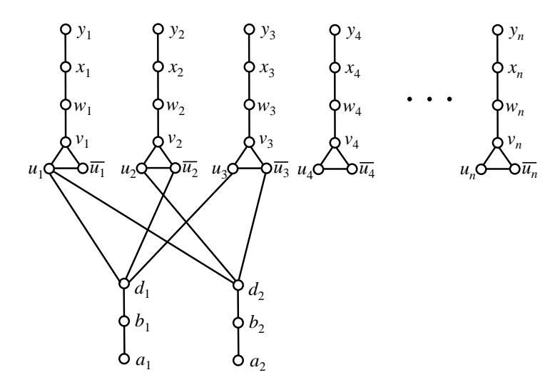
Figure 5. \(c_1 = \{u_1, \overline{u}_2, u_3\}, c_2 = \{u_1, u_2, \overline{u}_3\}, \text{ etc.}\)

Theorem 3.2. Simply deciding, for a given graph G, if G has an open-independent, OLD-set is an NP-complete decision problem. That is, XOIOLD is NP-complete.

Proof. One can easily verify in polynomial time if a given set \(S \subseteq V(G)\) is an \(OLD_{OIND}\)-set, so \(XOIOLD \in NP\).

We can reduce the known NP-complete 3-SAT problem to XOIOLD in polynomial time as follows. For each \(u_i \in U\) let \(G_i\) be the 6-vertex graph illustrated in Figure 5 with \(V(G_i) = \{u_i, \overline{u}_i, v_i, w_i, x_i, y_i\}\) and \(E(G_i) = \{u_i\overline{u}_i, u_iv_i, \overline{u}_iv_i, v_iw_i, w_ix_i, x_iy_i\}\). For each clause \(c_j \in C\) let \(H_j\) be the 3-vertex graph with \(V(H_j) = \{a_j, b_j, d_j\}\) and \(E(H_j) = \{a_jb_j, b_jd_j\}\). Interconnect the clause components and literal components by adding edges \(d_jc_{j,1}, d_jc_{j,2}\) and \(d_jc_{j,3}\) for \(1 \leq j \leq m\) where \(c_j = \{c_{j,1}, c_{j,2}, c_{j,3}\} \in C\), as illustrated in Figure 5. Let G be the resulting graph of order 6n + 3m.

Assume there is a satisfying truth assignment \(S\subseteq U\cup \overline{U}\). Form \(W\subseteq V(G)\) by letting \(\{y_i,x_i,v_i,a_j,b_j\}\subseteq W\) for \(1\leq i\leq n,\) \(1\leq j\leq m\). For \(1\leq i\leq n,\) add \(u_i\) to W if the literal \(u_i\in S\), otherwise the literal \(\overline{u}_i\in S\) and one adds \(\overline{u}_i\) to S. Then \(< W >\) consists of 4n+2m vertices inducing 2n+m independent edges. Note that \(N(a_j)=\{b_j\}\subseteq W,\) \(b_j\in N(d_j)\cap W\) but \(|N(d_j)\cap W|\geq 2\) because S is satisfying. It is easily seen that G has W as an open-independent, OLD-set.

Assume G has an \(OLD_{OIND}\)-set W. By Proposition 3.1 we have \(\{y_i, x_i\} \subseteq W\) with \(w_i \notin W\) for \(1 \leq i \leq n\), and \(\{a_j, b_j\} \subseteq W\) with \(d_j \notin W\) for \(1 \leq j \leq m\). Because \(N(y_i) \cap W = \{x_i\}\) and \(N(w_i) \cap W \neq N(y_i) \cap W\), each \(v_i \in W\). Now \(v_i \in W\) implies the open-independent, dominating set W has \(|N(v_i) \cap W| = 1\), so W contains exactly one of \(u_i\) and \(\overline{u}_i\). Let \(S = W \cap (U \cup \overline{U})\). Because W is an OLD-set \(N(a_j) \cap W = \{b_j\} \subsetneq N(d_j) \cap W\), and we have \(N(d_j) \cap (U \cup \overline{U}) \neq \emptyset\). That is, S must be a satisfying truth assignment.

Theorem 3.3. If the girth of G satisfies g(G) ≥ 5 and W ⊆ V (G), then W is an OLDOIND-set if and only if (1) each v ∈ W is open-dominated exactly once, and (2) each v /∈ W is open-dominated at least twice.

Proof. Assume W is an OLDOIND-set for G. Because W is open-independent and open-dominating, each v ∈ W has |N(v) ∩ W| = 1. If v /∈ W, then W open-dominates v implies there is a vertex w ∈ N(v) ∩ W. As noted |N(w) ∩ W| = 1, say N(w) ∩ W = {x}. Then N(x) ∩ W = {w} 6= N(v) ∩ W implies that |N(v) ∩ W| ≥ 2.

Assume conditions (1) and (2) hold for W ⊆ V (G). Then W is open-dominating. Assume v ∈ W has |N(v) ∩ W| = 1. For N(v) ∩ W = {w}, we have N(w) ∩ W = {v} and x ∈ N(w) − {v} implies that x /∈ W, so x is open-dominated at least twice. Thus v is the only vertex with N(v) ∩ W = {w}. Assume v /∈ W, let {x, y} ⊆ N(v) ∩ W. No other vertex u has {x, y} ⊆ N(u) ∩ W or else u, x, v, y is a 4-cycle and g(G) ≤ 4. Thus N(v) ∩ W uniquely distinguishes v.

Assume W is an OLDOIND-set for path Pⁿ : v1, v2, ..., vn. By Proposition 3.1 we have {v1, v2} ⊆ W, v³ ∈/ W, {v4, v5} ⊆ W, v⁶ ∈/ W, ...{vn−1, vn} ⊆ W.

Proposition 3.2. Path Pⁿ has an OLDOIND-set W if and only if n ≡ 2(mod 3) and OLDOIND(P3k+2) = 2k + 2.

Figure 6. Some trees with OLDOIND-sets.

Theorem 3.4. (Seo and Slater [26]) A tree T has an OLD-set if and only if no two endpoints of T have the same neighbor.

Similar to the characterization given in Studer, et al. [43] for open-independent dominating sets in trees, we can recursively define the collection of pairs (T, W) where T is a tree and W is the unique OLDOIND(T)-set. First note that the tree A^t of order 2t + 1 in Figure 6 has OLDOIND(At) = 2t and V (At) − x is the unique OLDOIND(At)-set for t ≥ 2.

Theorem 3.5. If Tⁿ is a tree of order n with an OLDOIND-set, then the OLDOIND(T)-set W is unique and Tⁿ can be obtained recursively from P² by a sequence of operations OP1 and OP2 defined as follows.

(OP1) Let T ^∗ be a tree with OLDOIND(T)-set W and let z ∈ W. The tree T is obtained from T ^∗ by adding a P³ : x, w, v and adding the edge zx.

(OP2) Let T ^∗ be a tree with OLDOIND(T)-set W and let z be any vertex in T ∗ . The tree T is obtained from T ^∗ by adding an A^t with t ≥ 2 and adding the edge zx.

Proof. We first observe that if T is obtained from T ^∗ by (OP1), then W ∪ {w, v} is an OLDOINDset for T, and if T is obtained from T ^∗ by (OP2), then W ∪ {w1, v1, ..., w^t , vt} is an OLDOIND-set for T.

Assume tree T has OLDOIND-set W. If T is a path, then Proposition 3.2 shows that T can be obtained from P² by a sequence of (OP1)-operations and there is a unique OLDOIND-set for T. If T is not a path, select a vertex y with deg y ≥ 3 where all or all but one of the branches at y are paths. Suppose y, u1, u2, ..., u^j is a branch path with j ≥ 3. By Proposition 1 we must have {uj−1, uj} ⊆ W and uj−² ∈/ W. Also uj−³ (possibly uj−³ = y) must be in W or else N(u^j )∩W = N(uj−2)∩W = {uj−1}. Let T ^∗ = T − {u^j , uj−1, uj−2}. Since W is an OLDOINDset of T and N(u^j ) ∩ V (T ∗ ) = ∅ and N(uj−1) ∩ V (T ∗ ) = ∅, W − {u^j , uj−1} is an OLDOIND-set of T ∗ . So T is obtainable from T ^∗ by (OP1) where z = uj−3. Because W is an OLD-set, y can not be the support vertex of two or more endpoints. If y is adjacent to an endpoint x and y, u1, u² is a branch path, Proposition 1 would imply that {u1, u2} ⊆ W and {x, y} ⊆ W, so W would not be open-independent. Now y can be assumed to have deg y − 1 = b branch paths of length two. We have a subgraph A^b with vertices {y, w1, v1, ..., wb, vb} with b ≥ 2. Let N(y) = {w1, w2, ..., wb, z}, and T can be obtained from T ^∗ = T − {y, w1, v1, ..., wb, vb} by (OP2).

4. OLDOIND% for infinite grids

Much work has been done on distinguishing sets (LD-sets, IC-sets and OLD-sets) in infinite grids (hexagonal, square, triangular, tumbling block, etc). See, for example, [1, 6, 7, 18, 19, 20, 22, 23, 26, 28, 29, 30, 40, 41].

For a given vertex x in a dominating set D in a graph G, the share sh(x; D) is defined in Slater [41] as a measure of how much domination the individual vertex x does. For example, in graph H1 of Figure 7 we have N[3] = {2, 3, 4, 5, 6, 9} and sh(3; {3, 4, 7}) = 1/2 + 1/2 + 1/2 + 1/3 + 1/2 + 1/3 = 8/3. Also, sh(4; {3, 4, 7}) = 1 + 1/2 + 1/2 + 1/2 + 1/3 + 1/2 + 1/3 = 11/3, and sh(7; {3, 4, 7}) = 1/3 + 1/2 + 1 + 1/2 + 1/3 = 8/3. Note that Σv∈Dsh(v; D) = |V (G)| = n for any dominating set D and that |D| ≥ |V (G)|/MAXv∈^V sh(v; D).

Similarly, the open share shop(x; D) is defined in Seo and Slater [26] for open dominating set D. Specifically, if D is open dominating and x ∈ D then, for each y ∈ N(x), let

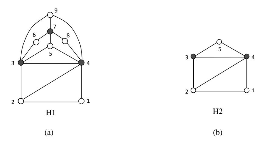
Figure 7. Graphs H¹ and H2.

shop(x; D(y)) = 1/|N(y) ∩ D| and let shop(x; D) = Σy∈N(x)shop(x; D(y)). For example, in Figure 7 D = {3, 4} is an open dominating set for the graph H2. We have N(3) = {2, 4, 5} and shop(3; D) = shop(3; D(2)) + shop(3; D(4)) + shop(3; D(5)) = 1/2 + 1 + 1/2 = 2. Also, N(4) = {1, 2, 3, 5} and shop(4; D) = shop(4; D(1)) + shop(4; D(2)) + shop(4; D(3)) + shop(4; D(5)) = 1 + 1/2 + 1 + 1/2 = 3. Note that Σx∈Dshop(x; D) = |V (G)|, and if shop(w; D) ≥ shop(x; D) for all x ∈ D, then |D| ≥ |V (G)|/shop(w; D).

In this paper, we will focus on open-locating-dominating sets along with open-shares of vertices.

Percentage parameters for measuring density for locally-finite, countably infinite graphs were defined in Slater [41]. For example, for the γ(G) parameter we have γ%(G) defined as follows as the minimum possible percentage of vertices in a dominating set of G. The closed k-neighborhood of vertex v is the set of vertices at distance at most k from v, N^k [v] = {w ∈ V (G) : d(v, w) ≤ k}. For S ⊆ V (G), the density of S is dens(S) = maxv∈^V (G) lim supk→∞(|S ∩ N^k [v]|/|N^k [v]|). Then, for example, the domination percentage of G is γ%(G) = min{dens(S) : S ⊆ V (G) is dominating}. Let HEX, SQ, and TRI denote the infinite hexagonal, square and triangular grid graphs, respectively.

Theorem 4.1. (Seo and Slater [26]) OLD%(HEX) = 1/2.

The darkened vertices of HEX in Figure 8 form an OLD%(HEX)-set D achieving the value 1/2, and D is an open-independent set. Hence we have the following.

Theorem 4.2. OLDOIND%(HEX) = OLD%(HEX) = 1/2.

Figure 9(a) illustrates that OLD%(SQ) = 2/5, but OLDOIND%(SQ) > OLD%(SQ).

Theorem 4.3. (Seo and Slater [26]) OLD%(SQ) = 2/5.

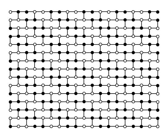
Figure 8. OLD%(HEX) = 1/2 = OLDOIND%(HEX).

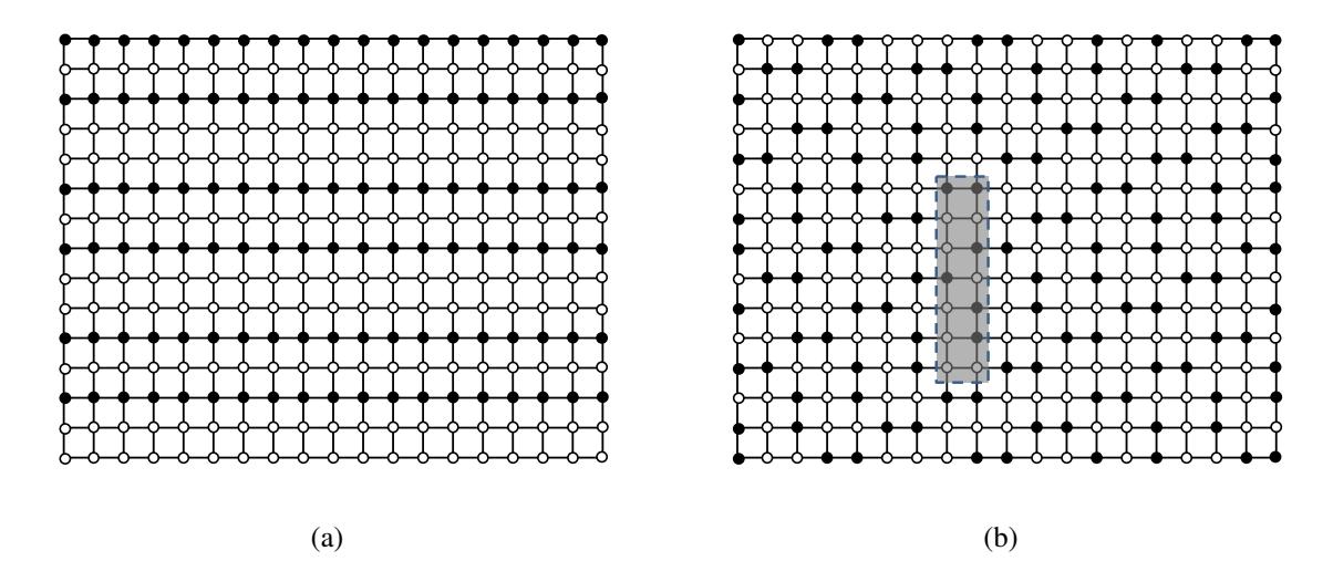
Figure 9. OLD%(SQ) = 2/5 and OLDOIND%(SQ) = 3/7.

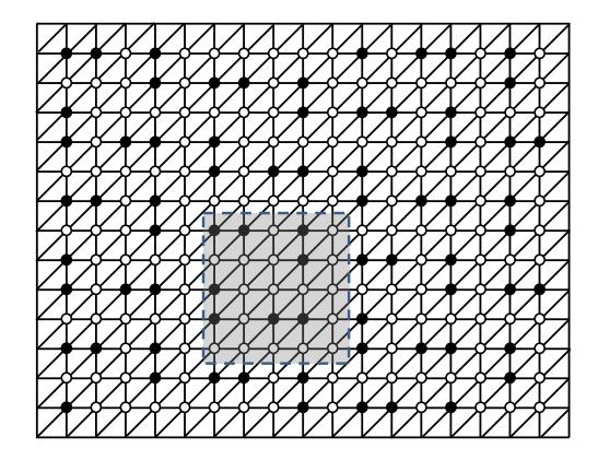
Figure 10. OLDOIND%(T RI) ≤ 8/25.

Theorem 4.4. OLDOIND%(SQ) = 3/7.

Proof. The set of darkened vertices in Figure 9(b) shows that OLDOIND%(SQ) ≤ 3/7. To see that OLDOIND%(SQ) ≥ 3/7 we use a straightforward share argument. Let D be an OLDOIND%(SQ) set. We have V (SQ) = Z × Z and N((i, j)) = {(i − 1, j),(i, j + 1),(i + 1, j),(i, j − 1)}. We will show that shop(x; D) ≤ 7/3 for every x ∈ D, and hence OLDOIND%(SQ) ≥ 7/3. Without loss of generality, assume x = (0, 0) ∈ D. Exactly one neighbor of x is also in D, and we can assume that (1, 0) ∈ D. In particular, shop(x; D((1, 0)) = 1. Any other vertex y ∈ N(x) is open dominated at least twice by D, so shop(x, D(y)) ≤ 1/2 for each y ∈ {(−1, 0),(0, 1),(0, −1)}. Suppose all three of these vertices give (0,0) a share value of 1/2.

Case 1. N((−1, 0))∩D = {(0, 0),(−2, 0)}. Then (−1, 1) ∈/ D with D∩{(−1, 0),(0, 1)} = ∅, and so N((−1, 1))∩D = {(−2, 1),(−1, 2)}. Similarly, N((−1, −1))∩D = {(−2, −1),(−1, −2)}. But then {(−2, 1),(−2, 0),(−2, −1)} ⊆ D, contradicting the open independence of D.

Case 2. N((−1, 0)) ∩ D 6= {(0, 0),(−2, 0)}. Then one of (−1, 1) and (-1,-1) is in D, say (-1, 1). Because shop((0, 0); D((0, 1)) = 1/2 we have N((0, 1)) ∩ D = {(0, 0),(−1, 1)}. Also, shop((0, 0); D((−1, 0)) = 1/2 implies N((−1, 0)) ∩ D = {(0, 0),(−1, 1)} = N(0, 1) ∩ D, contradicting the fact that D must distinguish (0,1) and (-1,0).

Because shop(x; D) < 1 + 1/2 + 1/2 + 1/2, we have shop(x; D) ≤ 1 + 1/2 + 1/2 + 1/3 = 7/3 for every x ∈ D. As noted, this implies OLDOIND%(SQ) ≥ 7/3.

Theorem 4.5. (Kincaid, Oldham, and Yu [23]) OLD%(T RI) = 4/13.

Figure 10 shows that OLDOIND%(T RI) ≤ 8/25. To date, the best we have is that: OLDOIND%(T RI) ∈ [4/13, 8/25].

5. Open independent sets

In this paper we focused on open-independence for OLD-sets. Of interest is the parameter OIND itself, as well as the lower open independence parameter oind where oind(G) is the minimum cardinality of a maximally open-independent set.

References

• [1] Y. Ben-Haim and S. Litsyn, Exact Minimum Density of Codes Identifying Vertices in the Square Grid. SIAM Journal on Discrete Mathematics 19 (2005), 69–82.
• [2] N. Bertrand, I. Charon, O. Hudry and A. Lobstein, Identifying and locating-dominating codes on chains and cycles, European Journal of Combinatorics 25 (2004), 969–987.
• [3] M. Blidia, M. Chellali, R. Lounes and F. Maffray, Characterizations of trees with unique minimum locating-dominating sets, Journal of Combinatorial Mathematics and Combinatorial Computing 76 (2011), 225–232.

• [4] M. Blidia, M. Chellali, F. Maffray, J. Moncel and A. Semri, Locating-domination and identifying codes in trees, Australasian Journal of Combinatorics 39 (2007), 219–232.
• [5] M. Chellali, N. J. Rad, S. J. Seo and P. J. Slater, On Open Neighborhood Locating-dominating in Graphs, Electronic Journal of Graph Theory and Applications 2 (2014), 87–98.
• [6] G.D. Cohen, I. Honkala, A. Lobstein and G. Zemor, Bounds for Codes Identifying Vertices ´ in the Hexagonal Grid, SIAM Journal on Discrete Mathematics 13 (2000), 492–504.
• [7] A. Cukierman and G. Yu, New bounds on the minimum density of an identifying code for the infinite hexagonal grid, Discrete Applied Mathematics 161 (2013), 2910–2924.
• [8] G. Exoo, V. Junnila and T. Laihonen, Locating-dominating codes in cycles, Australasian Journal of Combinatorics 49 (2011), 177–194.
• [9] F. Foucaud, R. Klasing, and P. J. Slater, Centroidal bases in graphs, Networks 64 (2014), 96–108.
• [10] M.R. Garey and D. S. Johnson, Computers and intractability: A guide to the theory of NPcompleteness, W.H. Freeman, (1979).
• [11] F. Harary and R. Melter, On the metric dimension of a graph, Ars Combinatoria 2 (1976), 191–195.
• [12] T.W. Haynes, S.T. Hedetniemi, and P.J. Slater, Fundamentals of Domination in graphs, Marcel Dekker, Inc., (1998).
• [13] T.W. Haynes, S.T. Hedetniemi, and P.J. Slater, Domination in Graphs: Advanced Topics, Marcel Dekker, Inc., (1998).
• [14] T.W. Haynes and P.J. Slater, Paired domination and the paired-domatic number, Congressus Numerantium 109 (1995), 67–72.
• [15] T.W. Haynes and P.J. Slater, Paired domination in graphs, Networks 32 (1998), 199–206.
• [16] M. Henning and A. Yeo, Distinguishing-transversal in hypergraphs and identifying open codes in cubic graphs, Graphs and Combinatorics Published online: 30 March 2013.
• [17] C. Hernando, M. Mora, and I. M. Pelayo, Nordhaus-Gaddum bounds for locating domination, European Journal of Combinatorics 36 (2014), 1–6.
• [18] I. Honkala, An optimal locating-dominating set in the infinite triangular grid, Discrete Mathematics 306 (2006), 2670–2681.
• [19] I. Honkala, An optimal strongly identifying code in the infinite triangular grid, Electronic Journal of Combinatorics 17 (2010), R91.

• [20] I. Honkala and T. Laihonen, On locating-domination sets in infinite grids, European Journal of Combinatorics 27 (2006), 218–227.
• [21] I. Honkala, T. Laihonen, and S. Ranto, On strongly identifying codes, Discrete Mathematics 254 (2002), 191–205.
• [22] M.G. Karpovsky, K. Chakrabarty and L.B. Levitin, On a new class of codes for identifying vertices in graphs, IEEE Transactions on Information Theory IT-44 (1998), 599–611.
• [23] R. Kincaid, A. Oldham, and G. Yu, On optimal open locating-dominating sets in infinite triangular grids, Mar 28 2014 math.CO arXiv:1403.7061v1
• [24] A. Lobstein, Watching systems, identifying, locating-dominating and discriminating codes in graphs, http://www.infres.enst.fr/ lobstein/debutBIBidetlocdom.pdf.
• [25] J. Moncel, On graphs on n vertices having an identifying code of cardinality dlog2(n + 1)e, Discrete Applied Mathematics 154 (2006), 2032–2039.
• [26] S.J. Seo and P.J. Slater, Open neighborhood locating-dominating sets, Australasian Journal of Combinatorics 46 (2010), 109–120.
• [27] S.J. Seo and P.J. Slater, Open neighborhood locating-dominating in trees, Discrete Applied Mathematics 159 (2011), 484–489.
• [28] S.J. Seo and P.J. Slater, Open neighborhood locating-domination for infinite cylinders, Proceedings of ACM SE (2011) 334–335.
• [29] S.J. Seo and P.J. Slater, Open neighborhood locating-domination for grid-like graphs, Bulletin of the Institute of Combinatorics and its Applications 65 (2012), 89–100.
• [30] S.J. Seo and P.J. Slater, Graphical parameters for classes of tumbling block graphs, Congressus Numerantium 213 (2012), 155–168.
• [31] S.J. Seo and P.J. Slater, Open locating-dominating interpolation for trees, Congressus Numerantium 215 (2013), 145–152.
• [32] S.J. Seo and P.J. Slater, OLD Trees with maximum degree three, Utilitas Mathematica 94 (2014), 361–380.
• [33] S.J. Seo and P.J. Slater, Fault Tolerant Detectors for Distinguishing Sets in Graphs, Discussiones Mathematicae Graph Theory, in press.
• [34] J.L. Sewell, Ph. D. Dissertation, in preparation.
• [35] J.L. Sewell and P.J. Slater, Fault tolerant identifying codes and locating-dominating sets, in preparation.
• [36] P.J. Slater, Leaves of trees, Congressus Numerantium 14 (1975), 549–559.

• [37] P.J. Slater, Domination and location in graphs, National University of Singapore, Research Report 93 (1983).
• [38] P.J. Slater, Dominating and location in acyclic graphs, Networks 17 (1987), 55–64.
• [39] P.J. Slater, Dominating and reference sets in graphs, Journal of Mathematical and Physical Sciences 22 (1988), 445–455.
• [40] P.J. Slater, Locating dominating sets and locating-dominating sets. Graph Theory, Combinatorics, and Applications: Proceedings of the 7th Quadrennial International Conference on the Theory and Applications of Graphs 2 (1995), 1073–1079.
• [41] P.J. Slater, Fault-tolerant locating-dominating sets, Discrete Mathematics 249 (2002), 179– 189.
• [42] P.J. Slater, Independent locating dominating sets and independent identifying codes, Submitted for publication.
• [43] D.S. Studer, T.W. Haynes, and L.M. Lawson, Induced-Paired Domination in Graphs, Ars Combinatoria 57 (2000), 111–128.