Luis R. Fuentesa , Italo J. Dejtera , Carlos A. Araujob
aUniversity of Puerto Rico, Rio Piedras, PR 00936-8377, Puerto Rico
luis.fuentes@upr.edu, italo.dejter@gmail.com, carlosaraujo@mail.uniatlantico.edu.co
Let 0 < n ∈ Z. In the unit distance graph of Z n ⊂ R n , a perfect dominating set is understood as having induced components not necessarily trivial. A modification of that is proposed: a rainbow perfect dominating set, or RPDS, imitates a perfect-distance dominating set via a truncated metric; this has a distance involving at most once each coordinate direction taken as an edge color. Then, lattice-like RPDS s are built with their induced components C having: (i) vertex sets V (C) whose convex hulls are n-parallelotopes (resp., both (n − 1)- and 0-cubes) and (ii) each V (C) contained in a corresponding rainbow sphere centered at C with radius n (resp., radii 1 and n − 2).
Keywords: perfect dominating set, lattice, tiling, rainbow sphere Mathematics Subject Classification : 05C69, 52C22, 11H31, 94B25
DOI: 10.5614/ejgta.2018.6.1.7
1. PRELIMINARIES
Before defining our main concerns in Section 2, we review perfect dominating sets and perfectdistance dominating sets, and sketch our plan.
1.1. Perfect Dominating Sets, (PDS s)
Let Γ = (V, E) be a graph and let S ⊂ V . Let [S] be the subgraph of Γ induced by S. The induced components of S, namely the connected components of [S] in Γ, are said to be the components of S. Several definitions of perfect dominating sets in graphs are considered in the
Received: 23 July 2016, Revised: 4 February 2018, Accepted: 21 February 2018.
bUniversidad del Atlantico, Barranquilla, Colombia ´
literature [23, 25]. We work with the following one [32] denoted with the short acronym PDS, to make a distinctive difference:
S is a PDS of \(\Gamma \Leftrightarrow\) each vertex of \(V \setminus S\) has a unique neighbor in S.
This definition (of PDS) differs from that of a 'perfect dominating set' as in [21, 22, 30] (that for us is a stable PDS coinciding with the perfect code of [4] or with the efficient dominating set of [3, 23]), in that [S] is not necessarily trivial.
Let \(0 < n \in \mathbb{Z}\). The following graphs are considered. The unit distance graph \(\Lambda_n^{\mathbb{R}}\) of \(\mathbb{R}^n\) has vertex set \(\mathbb{R}^n\) and exactly one edge between each two vertices if and only if their Euclidean distance is 1. Let \(\Lambda_n^{\mathbb{Z}}\) be the induced subgraph of \(\mathbb{Z}^n\) in \(\Lambda_n^{\mathbb{R}}\). If no confusion arises, we write \(\Lambda_n = \Lambda_n^{\mathbb{Z}}\) and express the elements \((a_1, \ldots, a_n) \in \mathbb{Z}^n\) with no parentheses or commas, namely as \(a_1 \cdots a_n\). This way, we denote: \(O = 00 \cdots 0\), \(e_1 = 10 \cdots 0\), \(e_2 = 010 \cdots 0\), ..., \(e_{n-1} = 0 \cdots 010\) and \(e_n = 00 \cdots 01\). An n-cube is the cartesian graph product \(Q_n = K_2 \square K_2 \square \cdots \square K_2\) of precisely n complete graphs \(K_2\). A grid graph is the cartesian graph product of two path graphs.
Our definition of a PDS S allows induced components of S in \(\Gamma\) which are not isolated vertices. For example: (a) tilings with generalized Lee r-spheres, for fixed r with \(1 < r \le n\) in \(\mathbb{Z}\) (e.g., crosses with arms of length one if r = n), furnish \(\Lambda_n\) with PDS s whose components are r-cubes [20]; (It is most remarkable that \(r = n \Leftrightarrow n \in \{2^r - 1, 3^r - 1; 0 < r \in \mathbb{Z}\}\) [6]); (b) total perfect codes [1, 26], that is PDS s whose components are \(K_2 = P_2\) in the \(\Lambda_n\) s and grid graphs; (these appear as diameter perfect Lee codes [19, 24]); (c) PDS s in n-cubes [5, 12, 13, 15, 16, 32], where \(0 < n \in \mathbb{Z}\), including the perfect codes of [18]; (d) PDS s in grid graphs [13, 26].
1.2. Perfect-Distance Dominating Sets
In [2], an extension of the definition of PDS is given as follows. Let \(t \ge 1\) and \(\Gamma = (V, E)\) be a graph. A set \(S \subset V\) is a t-perfect-distance dominating set (t-PDDS) in \(\Gamma\) if, for each \(v \in V\), there is a unique component \(C_v\) of S so that for the graph distance \(d(v, C_v)\) from v to \(C_v\) it is \(d(v, C_v) \le t\), and there is in \(C_v\) a unique vertex w with \(d(v, w) = d(v, C_v)\).
We refer to [2] for relations of PDDS s to other domination and coding notions. For \(0 < n \in \mathbb{Z}\), the tilings with generalized Lee spheres of [20] (see Subsection 1.2 item (a)) provide \(\Gamma = \Lambda_n\) with t-PDDS s whose components are r-cubes, for any fixed \(t \in \mathbb{Z}\) and \(r \in \mathbb{Z}\) such that \(t \geq 1\) and \(0 \leq r \leq n\).
1.3. Plan of the Paper and Related Motivation
In Section 2, rainbow perfect dominating sets, or RPDS s, are defined that generalize PDS s while imitating the definition of PDDS but using a truncated metric [17], pages 40 and 262. This has a rainbow distance by coloring the edges of \(\Lambda_n^{\mathbb{Z}}\) according to the n coordinates, for \(0 < n \in \mathbb{Z}\). With the aim of packing perfectly the resulting rainbow spheres, Section 3 takes to the construction of lattice-like RPDS s S whose induced graphs [S] have their components C possessing: (i) vertex sets with n-parallelotopes as their convex hulls in \(\mathbb{R}^n\) and minimal separating graph distance 3, having a set of representatives that forms a lattice with generating elements precisely along the coordinate directions of \(\mathbb{Z}^n\) and (ii) each V(C) contained in a corresponding rainbow sphere centered at C with radius n.
It is not clear that similar lattice-like results hold with r-parallelotopes (0 < r < n), including lattice-like rainbow total perfect codes (case r = 1). However, once the concept of lattice-like is generalized in Section 4, we are able to show that a lattice-like RPDS S exists in Λn whose [S] has its components C possessing: (i′ ) vertex sets with (n − 1)- and 0-cubes as their convex hulls in R n and (ii′ ) each V (C) contained in a corresponding rainbow sphere centered at C with respective radii 1 and (n − 2).
Motivation for this outcome of RPDS s with induced components that are r-cubes of different dimensions r (Theorem 4.2) comes both from the perfect covering codes with spheres of two different radii in Chapter 19 of [11] and from a negative answer to a conjecture [32] claiming that the components of a PDS S in an n-cube Qn are r-cubes Qr where r is fixed with 0 ≤ r ≤ n. In fact, it was found in [31] that a PDS in Qn with components that are r-cubes Qr in Q13 of two different dimensions r = r1 and r = r2 exist, specifically with r1 = 4 and r2 = 0. However, this is still the only known counterexample to the conjecture of [32].
2. RAINBOW PERFECT DOMINATING SETS
Let 0 < n ∈ Z. Let Γ = (V, E) be a graph edge-colored in In = {1, . . . , n}. A path Pe in Γ is a rainbow path if no color appears more than once in Pe [8, 9, 10, 27, 28, 29]. We consider a truncated metric that generalizes that of [17], pages 40 and 262 and is defined between two vertices u and v in Γ by their rainbow distance ρ(u, v), namely: (i) the shortest length of a rainbow path Pe joining u and v, if such Pe exists; (ii) |In|+1 = n+1, otherwise. Notice that ρ is not a well-defined distance like the graph distance d of Γ given by the shortest length d(u, v) of a path P between u and v. If K is a component of S and u ∈ V then we denote ρ(u, K) = min{ρ(u, v); v ∈ K} and d(u, K) = min{d(u, v); v ∈ K}. Let 1 ≤ t ≤ n. A set S ⊆ V is said to be a t-rainbow perfect dominating set or t-RPDS in Γ if for each v ∈ V there are: (a) a unique component Kv of S with ρ(v, Kv) ≤ t and (b) a unique vertex w in Kv with ρ(v, w) = ρ(v, Kv). If in this definition of t-RPDS we replace ρ by d then S becomes a t-PDDS in Γ, as in [24].
Let H = (V, E) be a subgraph of Λn and let z ∈ Z n . Then H + z denotes the graph H′ = (V ′ , E′ ) with vertex set V ′ = V + z = {w ∈ Z n ; ∃ v ∈ V such that w = v + z} and such that uv ∈ E if and only if (u + z)(v + z) ∈ E ′ . Observe that the subgraph H of Λn induced by the set of vertices with entries in {0, 1} (and by extension any translation H′ = H + z of such an H in Λn) constitutes an n-cube Qn.
Let i ∈ In. Each edge of Λn parallel to Oei is assigned color i. Thus, an edge uv of Λn has color i if and only if u−v ∈ {±ei}. Considering this for every i ∈ In, Λn becomes an edge-colored graph having its copies of the n-cube Qn as its largest properly edge-colored subgraphs.
All 1-RPDS s are PDS s. A PDS is both a 1-RPDS and a 1-PDDS, so that 1-RPDS s and 1- PDDS s coincide as PDS s. However, this is not the case if t > 1. The following restriction of a theorem of [32] (Theorem 1 of [2] has a similar proof) is expressed in terms of monochromatic paths in the edge-colored Λn with a monochromatic path understood as either one-way infinite or two-way infinite or having length either null or positive.
Theorem 2.1. If S is a t-RPDS in Λn then each component of S is the cartesian product of monochromatic paths of different colors in Λn.
Let J be a cartesian product of finite monochromatic paths of different colors in \(\Lambda_n\). The rainbow sphere \(W_{n,J,t}^{\rho}\) of radius t around J in \(\Lambda_n\) is the union of V(J) and the set of those \(v \in \mathbb{Z}^n\) with \(\rho(v,V(J)) \leq t\). Here, J is said to be the rainbow center of \(W_{n,J,t}^{\rho}\). The graph sphere \(W_{n,J,t}^d\) is defined similarly and has J as its corresponding graph center. If there is no confusion, we drop the initial adjective rainbow or graph. If J is an r-cube, where \(0 \leq r \leq n\), then we write \(W_{n,J,t}^{\rho} = W_{n,r,t}^{\rho}\) and \(W_{n,J,t}^{d} = W_{n,r,t}^{d}\). It is seen that \(W_{n,J,t}^{\rho}\) is a generalized Lee spheres [20]. Figure 1 represents two rainbow spheres (dark gray) in \(\Lambda_2\) contained in respective graph spheres (twotone gray), namely \(W_{2,0,2}^{\rho}\) (dark gray) \(\subset W_{2,0,2}^{d}\) (two-tone gray) and \(W_{2,1,2}^{\rho}\) (dark gray) \(\subset W_{2,1,2}^{d}\) (two-tone gray).
Figure 1. Rainbow spheres contained in respective graph spheres.
A t-RPDS S of \(\Lambda_n\) determines a partition of \(\mathbb{Z}^n\) into the spheres \(W_{n,K,t}^{\rho}\), with K running over the components of S. A t-PDDS S' of \(\Lambda_n\) determines similarly a partition of \(\mathbb{Z}^n\) into the spheres \(W_{n,K',t}^d\), with K' running over the components of [S'].
A t-RPDS S in \(\Lambda_n\) such that the components of S are all isomorphic to a fixed finite graph H is said to be a t-RPDS[H]. Let S be a t-RPDS[H] and let K be a component of S with K isomorphic to H. Then S is said to be lattice-like ([2]) if: there is a lattice \(L \subseteq \mathbb{Z}^n\) such that K' is a component of S if and only if K' = K + z with \(z \in L\). A set \(S \subset \mathbb{Z}^n\) is periodic [2] if there are integers \(p_1, \ldots, p_n\) such that \(v \in S\) implies \(v \pm p_i e_i \in S\) for all \(i = 1, \ldots, n\). Notice that each lattice-like t-RPDS[H] S is periodic [2]. Thus, a suitable restriction of such an S yields a t-RPDS[H] in a cartesian product of n cycles \(C_{k_1p_1} \square C_{k_2p_2} \square \cdots \square C_{k_np_n}\) with \(0 < k_i \in \mathbb{Z}\), for \(i = 1, 2, \ldots, n\). This observation is easily adapted to the generalizations of a t-RPDS[H] below, up to Section 4. In fact, the second parts of the statements of Theorems 3.1, 4.1 and 4.2 use them. However, we prove just the existence of those RPDS s in the \(\Lambda_n\) s, leaving the covering and projection (onto cartesian products of cycles) parts of the proofs to the reader.
Let H be a cartesian product of finite monochromatic paths of different colors in \(\Lambda_n\). If just r elements of \(I_n\) color the edges of H, then we say that H is an r-box. In this case, H is a cartesian product \(\prod_{i=1}^n P_i\) where \(P_i\) is a finite path, for \(1 \le i \le n\), with exactly r paths \(P_i\) having positive length. Clearly, the convex hull of an r-box is an r-parallelotope and any r-cube in \(\Lambda_n\) is an r-box, for \(0 \le r \le n\)..
A constellation of a lattice L in \(\mathbb{Z}^n\) is a subset \(T \subseteq \mathbb{Z}^n\) that contains exactly one vertex from each class mod L so that T is in fact a complete system of coset representatives of L in \(\Lambda_n\). (Compare with fundamental region, [7], pg. 26). We still say that a partition of \(\mathbb{Z}^n\) into constellations of L is a tiling of \(\mathbb{Z}^n\) and that those constellations are its tiles.
3. TOP RADIUS AND BOX DIMENSION
A particular case of t-RPDS[H] is that in which H is an n-box in \(\Lambda_n\). For each such n-box H we show that there is a lattice-like RPDS[H] in \(\Lambda_n\). (In [6], n-boxes of unit volume in \(\Lambda_n\) are shown to determine 1-PDDS[H] s if and only if either \(n=2^r-1\) or \(n=3^r-1\)).
Theorem 3.1. For each n-box \(H = \prod_{i=1}^n P_i\) in \(\Lambda_n\), where \(P_i\) is a path of color i and length \(\ell_i\) \((i=1,\ldots,n)\), there exists a lattice-like n-RPDS[H] S of \(\Lambda_n\). This S covers an n-RPDS[H] in any cartesian product of cycles \(C_{(\ell_1+3)k_1} \square C_{(\ell_2+3)k_2} \square \cdots \square C_{(\ell_n+3)k_n}\) with \(1 < k_i \in \mathbb{Z}\) \((i=1,\ldots,n)\). The minimum graph distance between the induced components of S is S.
Proof. Assume S is an n-RPDS[H] in \(\Lambda_n\). As already commented, S determines a partition of \(\mathbb{Z}^n\) into the spheres \(W_{n,K,n}^{\rho}\) with K running over the components (isomorphic to H) of S. These spheres conform a tiling which is associated to a lattice \(L_S\) to be set now. In each such \(W_{n,K,n}^{\rho}\) let \(b_1b_2\cdots b_n\) be the vertex \(a_1a_2\cdots a_n\) for which \(a_1+a_2+\cdots +a_n\) is minimal. We say that this \(b_1b_2\cdots b_n\) is the anchor of \(W_{n,K,n}^{\rho}\). Then the anchors of the spheres \(W_{n,K,n}^{\rho}\) form the lattice \(L=L_S\). Without loss of generality we can assume that O is the anchor of a \(W_{n,H_0,n}^{\rho}\) whose center \(H_0\) is a component of S isomorphic to H. In \(W_{n,H_0,n}^{\rho}\) let \(c_0c_1\cdots c_n\) be the vertex \(a_1a_2\cdots a_n\) in \(W_{n,H_0,n}^{\rho}\) for which \(a_1+a_2+\cdots a_n\) is maximal. Then \(L_S\) has generating set \(\{(1+c_1)e_1, (1+c_2)e_2, \ldots, (1+c_n)e_n\}\) and is formed by all linear combinations of its elements. This insures that S exists and is lattice-like via \(L_S\). Remaining details of the proof are left to the reader, who must check that \(\ell_i=c_i-2\), for \(i=1,\ldots,n\).
Theorem 3.1 can be proved alternatively by the additive-group epimorphism technique [2, 1, 24] modified in Section 5 as Proposition 5.1. Figure 3 in Section 4 below suggests in light-gray color at least two induced components of a t-RPDS[H] in \(\Lambda_n\) as in Theorem 3.1, where t=3, \(H=Q_0\) and n=3.
The Voronoi diagram of \(\mathbb{Z}^n\) in \(\mathbb{R}^n\) has its composing Voronoi regions ([7], pg. 26) as the unit-volume n-dimensional cubes, cartesian product \(\prod_{i=1}^n [a_i - \frac{1}{2}, a_i + \frac{1}{2}]\). Let \(H_0\) and L be as in the proof of Theorem 3.1. Consider the vertices v of a sphere \(W_{n,H_0,n}^{\rho} + \ell\), (\(\ell \in L\)). The union of the Voronoi regions of those v is called the Voronoi box \(B_{n,H_0,n,\ell}^{\rho}\) of \(W_{n,H_0,n}^{\rho} + \ell\). Then, \(\mathbb{R}^n\) admits a Voronoi partition \(\mathcal V\) into constellations (in a way similar to that of [7], pg.26) each contained in a corresponding Voronoi box \(B_{n,H_0,n,\ell}^{\rho}\) but containing its anchor in \(L = L_S\) and just one point from each pair of antipodal points in its boundary (equidistant from the barycenter of \(B_{n,H_0,n,\ell}^{\rho}\) along a straight line). As a result, \(L = L_S\) is a set of representatives of \(\mathcal V\), but \(\mathcal V\) is not uniquely defined.
Corollary 3.1. For each n-box H, \(\mathbb{R}^n\) admits a Voronoi partition into constellations associated to the Voronoi boxes \(B_{n,H_0,n,\ell}^{\rho}\) where both \(H_0\) and L are as in the proof of Theorem 3.1, and \(\ell\) runs over L.
4. SMALLER RADII AND BOX DIMENSIONS
Existing results of lattice-like t-RPDS s in \(\Lambda_n\) with t < n concern solely t = 1 (that is for PDS s). In fact, constructions in [2, 6, 20, 24] lead to lattice-like 1-RPDS. However, it seems that
there are not many of these 1-RPDS s. For example, [14] shows that there is only one lattice-like 1-RPDS[\(Q_2\)] and no 1-RPDS[\(Q_2\)] which is not lattice-like. In contrast with the existence of a lattice-like 2-PDDS[\(P_2\)] in \(\Lambda_3\) arising from a Minkowsky tiling cited in [2], we may combine the conjecture in Subsection 1.3 with the related conjecture that there are no lattice-like t-RPDS in \(\Lambda_n\), for 1 < t < n.
Figure 2. Constellation of a lattice \(L_S\) for a 1-RPDS[\(Q_1\); 4] S in \(\Lambda_3\).
If S is a periodic t-RPDS[H] in \(\Lambda_n\) and is not lattice-like, then for some positive integer m there is a tiling of \(\Lambda_n\) with tiles that are the vertex set of a connected subgraph \(H^*\) induced in \(\Lambda_n\) by the union of both: (a) m disjoint copies \(H^1, \ldots, H^m\) of H that intervene as components of S and (b) the set formed by the vertices \(v \in \mathbb{Z}^n\) for which \(\rho(v, H^j) \leq t\), for some \(j \in I_m\). If so, by taking m as small as possible, we say that S is a t-RPDS[H; m].
For example, Section 5 of [2] shows the existence of a 1-RPDS[\(Q_1\); 4] S which is not lattice-like. However, there exists a lattice \(L_S\) based on such S with each of its constellations containing two copies of \(Q_2\) in color 1 (of edge \(Oe_1\)) and two copies of \(Q_1\) in color 2 (of edge \(Oe_2\)), all four copies of \(Q_2\) being components of S. This is represented in Figure 2, where the rainbow 1-spheres of such four components (in thick trace) are shaded dark gray and the remaining area completing their convex hull is in light gray.
Here we can take a fixed vertex \(v_T\) in each resulting tile T so that all the vertices \(v_T\) constitute the lattice \(L_S\). Thus, even for a non-lattice-like t-RPDS we can recover a lattice formed by selected vertices \(v_T\) in the corresponding tiles T associated to S. However, when describing S as a t-RPDS[H;m], we can say that S is a lattice-like t-RPDS[H;m] as there is indication between brackets of the components of S in a resulting typical tile T in which to fix a sole distinguished vertex \(v_T\) so that all such distinguished vertices constitute a lattice \(L_S\) and the resulting tiling is effectively a lattice-like tiling. We generalize this situation as follows.
A t-RPDS S in \(\Lambda_n\) with the components of S isomorphic to two different fixed finite graphs \(H_0\) and \(H_1\) is said to be a t-RPDS\([H_0, H_1]\). Even though such an S cannot be lattice-like, it may happen that there exists a lattice \(L_S\) such that for some positive integers \(m_0\) and \(m_1\) there exists a constellation of \(L_S\) in \(\Lambda_n\) given by the union of two disjoint subgraphs \(H_0^*\) and \(H_1^*\), where \(H_i^*\) (i=0,1) is induced in \(\Lambda_n\) by the disjoint union of: (a) \(m_i\) copies \(H_i^1,\ldots,H_i^{m_i}\) of \(H_i\) that intervene as components of S and (b) the sets of vertices \(v \in \mathbb{Z}^n\) for which \(0 < \rho(v,H_i^j) \le t\), for \(j \in I_{m_i}\). In this case, S is said to be a lattice-like t-RPDS\([H_0,H_1;m_0,m_1]\). We can take a fixed vertex \(v_T\) in each resulting tile T so that all the vertices \(v_T\) form the lattice \(L_S\). We obtain a 1-RPDS\([H_0,H_1;m_0,m_1]\) in the following statement, where \(H_0=Q_2,H_1=Q_0,m_0=2,m_1=2\),
Figure 3. Elements of a constellation for a 1-RPDS[\(Q_2, Q_0; 2, 2\)] in \(\Lambda_3\).
with a constructive proof of it in Section 6 by means of Proposition 5.1.
Theorem 4.1. There exists a lattice-like 1-RPDS \([Q_2, Q_0; 2, 2]\) S in \(\Lambda_3\). This S covers a 1-RPDS \([Q_2, Q_0; 2, 2]\) of any cartesian product \(C_{6k_1} \square C_{6k_2} \square C_{3k_3}\) with \(0 < k_i\), for i = 1, 2, 3. The minimum graph distance between the induced components \(Q_2\) (resp., \(Q_0\)) of S is 3.
This is represented in Figure 3, where the components of S in one of the constellations of \(L_S\) formed by two copies of \(Q_2\) and two copies of \(Q_0\), are blackened and the edges in the rainbow 1-spheres having them as centers are shown in dark trace; the other edges induced in the union of these four components are in dark-gray trace. For better reference, the rainbow 3-spheres of the 3-RPDS\([Q_0]\) resulting from Theorem 3.1 are shaded in light gray. Also, dark gray was used to indicate two other copies of \(Q_2\) appearing in the figure that are components of S. Notice that vertices \(O, e_1, e_2, e_3\) are indicated in the figure. The minimum distance between the induced components \(Q_{n-1}\) (resp., \(Q_0\)) of S is 3.
More generally, let \(1 \le t_i \le n\), for i = 0, 1. A set \(S \subset V\) is said to be a \((t_0, t_1)\)-RPDS\([H_0, H_1]\) in \(\Lambda_n\) if for each \(v \in V\) there is: (i) a unique index \(i \in \{0, 1\}\) and a unique component \(K_v^i\) of S such that the distance \(\rho(v, K_v^i)\) from v to \(C_K^i\) satisfies \(\rho(v, K_v^i) \le t_i\) and (ii) there is a unique vertex w in \(K_v^i\) such that \(\rho(v, w) = \rho(v, K_v^i)\).
Even though such an S cannot be lattice-like, it may happen that there exists a lattice \(L_S\) such that for some positive integers \(m_0\) and \(m_1\) there exists a constellation of \(L_S\) in \(\Lambda_n\) given by the union of two disjoint subgraphs \(H_0^*\) and \(H_1^*\), where \(H_i^*\) (i=0,1) is induced in \(\Lambda_n\) by the disjoint union of: (a) \(m_i\) disjoint copies \(H_i^1, \ldots, H_i^{m_i}\) of \(H_i\) that intervene as components of S and (b) the sets of vertices \(v \in \mathbb{Z}^n\) for which \(0 < \rho(v, H_i^j) \le t_i\), for \(j \in I_{m_i}\). In this case, S is said to be a lattice-like \((t_0, t_1)\)-RPDS\([H_0, H_1; m_0, m_1]\). We can take a fixed vertex \(v_T\) in each resulting tile T so that all the vertices \(v_T\) form a lattice \(L_S\). A family of lattice-like \((t_0, t_1)\)-RPDS\([H_0, H_1; m_0, m_1]\) s in the lattices \(\Lambda_n\) that extend the 1-RPDS\([Q_2, Q_0; 2, 2]\) of Theorem 4.1 is obtained as follows, where
\(H_0 = Q_{n-1}\), \(H_1 = Q_0\), \(m_0 = m_1 = 2\), \(t_0 = 1\), \(t_1 = n - 2\), with a constructive proof of it in Section 7.
Theorem 4.2. There exists a lattice-like (1, n-2)-RPDS\([Q_{n-1}, Q_0; 2, 2]\) S in \(\Lambda_n\). This S covers a (1, n-2)-RPDS\([Q_{n-1}, Q_0; 2, 2]\) in any cartesian product \(C_{6k_1} \square ... \square C_{6k_{n-1}} \square C_{3k_n}\) with \(0 < k_i\), for i = 1, ..., n.
5. ADDITIVE-GROUP EPIMORPHISMS
All the constructions of RPDSs mentioned in this paper can be confirmed by means of the additive-group epimorphism technique presented in this section. In fact, we use a modification of Corollary 2 in [2] in the following two sections. This is a corollary to Theorem 6 [24] whose proof uses the linear-algebraic notion of translation of subsets \(S \subset \mathbb{Z}^n\). The modification in question (of the corollary) is given as Proposition 5.1 below and it is tailored in order to complete the proofs of the results in Section 4. The additive-group epimorphism technique starts by having:
- (a) a lattice L in \((\mathbb{Z}^n, +)\) generated by elements \(u_1, \ldots, u_n \in \mathbb{Z}^n\) such that \(L = \{\alpha_1 u_1 + \ldots + \alpha_n u_n; \alpha_i \in \mathbb{Z}, i = 1, \ldots, n\}\);
- (b) a set \(T \subseteq \mathbb{Z}^n\) containing one element from each coset of \(\mathbb{Z}^n \mod L\) such that \(\{T+u : u \in L\}\) is a partition of \(\mathbb{Z}^n\) into subsets of size \(|\mathbb{Z}^n/L|\), with the induced subgraphs [T+u] of T+u in \(\Lambda_n\) pairwise isomorphic, where \(u \in L\).
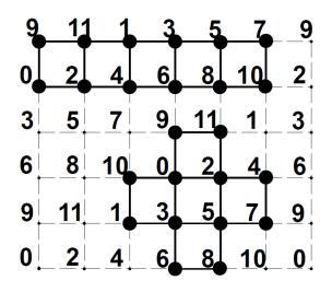
Figure 4. Accompanying example: two possible selections for [T].
Given a lattice L, we can split \(\mathbb{Z}^n\) into subsets with their induced subgraphs having different shapes depending on the choice of T. For example, \(L = \{\alpha_1(3,2) + \alpha_2(0,4); \alpha_i \in \mathbb{Z}, i = 1,2\}\) in \(\Lambda_2\) has \((\mathbb{Z}^n,+)/L = \mathbb{Z}_{12}\). The graph [T] might be either the cartesian product \(P_6 \square P_2\) or the closed neighborhood of a 2-cube \(Q_2 = P_2 \square P_2\), as shown in Figure 1.
Let D=(V,E) be an induced subgraph of \(\Lambda_n\). We are looking for a partition (tiling) of \(\Lambda_n\) into copies of D. We need to find a lattice L for the required selection of the set T with [T]=D. The following construction leads to the sought tiling of \(\Lambda_n\).
If there is an abelian group (G, +) of order |V| and elements \(g_1, \ldots, g_n\) of G such that the restriction of the epimorphism \(\Phi : \mathbb{Z}^n \to G\) defined by \(\Phi((a_1, \ldots, a_n)) = a_1 \Phi(e_1) + \ldots + a_n \Phi(e_n) = a_1 g_1 + \ldots + a_n g_n\) to V is a bijection then there is a partition of \(\Lambda_n\) into copies of D.
In other words, we need to find an abelian group G of order |V| and assign elements \(g_1, \ldots, g_n\) of G to the vertices \(e_1, \ldots, e_n\) of \(\Lambda_n\) such that \(\Phi((a_1, \ldots, a_n)) = a_1 \Phi(e_1) + \ldots + a_n \Phi(e_n) = a_1 \Phi(e_1) + \ldots + a_n \Phi(e_n)\)
\(a_1g_1+\ldots+a_ng_n\) is a bijection on V. Since the kernel of a group epimorphism \(\Phi:\mathbb{Z}^n\to G\) is a subgroup of \(\mathbb{Z}^n\), then the elements w of \(\mathbb{Z}^n\) for which \(\Phi(w)=0\) form a lattice L in \((\mathbb{Z}^n,+)\). In addition, \((\mathbb{Z}^n,+)/L=G\); also, V has exactly one element in each coset of \((\mathbb{Z}^n,+)/L\). Thus we can set T=V.
TABLE I
| \(\mathbb{Z}^3\) | \(| \stackrel{\to}{\Phi}\) | G | |||||||||||||
|---|---|---|---|---|---|---|---|---|---|---|---|---|---|---|---|
| ••• | ••• | 122 | 222 | ••• | ••• | ••• | ••• | ••• | 322 | 422 | ••• | ••• | ••• | ••• | |
| ••• | ••• | 112 | 212 | ••• | ••• | ••• | ••• | ••• | 212 | 312 | ••• | ••• | ••• | ••• | |
| ••• | ••• | 131 | 231 | ••• | ••• | ••• | ••• | ••• | ••• | 401 | 501 | ••• | ••• | ••• | ••• |
| ••• | 021 | 121 | 221 | 321 | ••• | ••• | ••• | 221 | 321 | 421 | 521 | ••• | ••• | ••• | |
| ••• | 011 | 111 | 211 | 311 | ••• | ••• | ••• | 111 | 211 | 311 | 411 | ••• | ••• | ••• | |
| ••• | 001 | 101 | 201 | 301 | ••• | ••• | ••• | 001 | 101 | 201 | 301 | ••• | ••• | ••• | |
| ••• | ••• | 120 | 220 | ••• | 420 | 520 | ••• | ••• | ••• | 320 | 420 | ••• | 020 | 120 | ••• |
| ••• | 010 | 110 | 210 | 310 | 410 | 510 | ••• | 110 | 210 | 310 | 410 | 510 | 010 | ••• | |
| 1-00 | 000 | 100 | 200 | 300 | 400 | ••• | ••• | |500| | 100 | 200 | 300 | 400 | ••• | ••• | |
| ••• | 01-0 | ••• | ••• | 31-0 | ••• | ••• | ••• | ••• | 520 | ••• | ••• | 220 | ••• | • • • | ••• |
| ••• | ••• | ••• | ••• | ••• | 531- | ••• | ••• | ••• | ••• | ••• | ••• | 102 | 202 | ••• | |
| ••• | ••• | ••• | ••• | 321- | 421- | 521- | 621- | ••• | ••• | ••• | 522 | 022 | 122 | 222 | |
| ••• | ••• | ••• | ••• | 311- | 511- | 611- | | | ••• | ••• | ••• | 412 | 012 | 112 | ||
| ••• | 001 | ••• | ••• | 301- | 501- | ••• | ••• | 002 | ••• | ••• | 302 | 402 | 502 | ••• | |
| ••• | ••• | ••• | ••• | ••• | 422 | 522 | ••• | ••• | ••• | ••• | ••• | ••• | 021 | 121 | ••• |
| ••• | ••• | ••• | ••• | ••• | 412 - | 512 - | ••• | ••• | ••• | ••• | ••• | ••• | 511 | 011 | ••• |
As mentioned, Corollary 2 of [2] can be modified as follows.
Proposition 5.1. Let \(1 \le t_i \in \mathbb{Z}\) and \(1 \le m_i \in \mathbb{Z}\). Let \(H_i\) be a finite subgraph of \(\Lambda_n\), for i=0,1. Let H be the disjoint union in \(\Lambda_n\) of \(m_0\) copies of \(H_0\) and \(m_1\) copies of \(H_1\). Let an induced supergraph \(H^*\) of H in \(\Lambda_n\) be such that a vertex v is in \(H^*\) if and only if there is just a copy H' of \(H_i\) that is a component of H with the least \(\rho(v,H') \le t_i\), for a fixed i=0,1 dependent only on v. Let D=(V,E) be a copy of \(H^*\) in \(\Lambda_n\) that contains vertices \(O,e_1,\ldots,e_n\). Then there is a lattice-like \((t_0,t_1)\)-RPDS\([H_0,H_1;m_0,m_1]\) if there exists an abelian group G of order |V| and a group epimorphism \(\Phi:\mathbb{Z}^n\to G\) such that the restriction of \(\Phi\) to V is a bijection.
6. PROOF OF THEOREM 4.1
If x < y in \(\mathbb{Z}\), then let \([x,y] = \{z \in \mathbb{Z}; x \le z \le y\}\). Consider the subset \(X \subset \mathbb{Z}^3\) of vertices of \(\Lambda_3\) whose coordinates are divisible by 3. Clearly, X is a lattice of \(\mathbb{Z}^3\). Each element of X is in a subset \(\tau_{x_1,x_2,x_3} = [3x_1,2+3x_1] \times [3x_2,2+3x_2] \times [3x_3,2+3x_3]\) of \(\mathbb{Z}^3\), with \(x_1,x_2,x_3 \in \mathbb{Z}\). Such a subset is a constellation of the lattice X and from now on will be called a 3-grenade.
TABLE II
0011- | 0110 0010 0110 | 1010 | 0011 | ||||||
|---|---|---|---|---|---|---|---|---|---|
| \(\mathbb{Z}^4\) | 1-001- | 0101- 0001- 01-01- | 1001- | 1-100 1-000 1-1-00 | 0100 0000 0100 | 1100 1000 1+00 | 1-001 | 0101 0001 0101 | 1001 |
001-1- | 1-01-0 | 011-0 001-0 01-10 | 101-0 | 001-1 | |||||
| \(\overline{\downarrow^{\Phi}}\) | |||||||||
| • | 1012 | 0010 | 2110 1010 0210 | 2010 | 1011 | ||||
| G | 5002 | \[\begin{array}{c} 1102 \\ 0002 \\ 5202 \end{array}\] | 1002 | 0100 5000 4200 | 1100 0000 5200 | \(2100 \\ 1000 \\ 0200\) | 5001 | \(1101 \\ 0001 \\ 5201\) | 1001 |
5022 | 4020 | 0120 5020 4220 | 0020 | 5021 |
A lattice-like 1-RPDS\([Q_2,Q_0;2,2]\) as claimed in Theorem 4.1 is composed by X and a subset Y defined as follows. We select in each 3-grenade \(\tau_{x_1,x_2,x_3}\) the 2-cube (or square) \(\sigma_{x_1,x_2,x_3}=[1+3x_1,2+3x_1]\times[1+3x_2,2+3x_2]\times\{1+\delta+3x_3\}\), where \(\delta\) is the rest of dividing \(x_1+x_2\) by 2. Then Y is given by the union of all squares \(\sigma_{x_1,x_2,x_3}\) with \(x_1,x_2,x_3\in\mathbb{Z}\). Theorem 4.1 is a direct corollary of the following lemma.
Lemma 6.1. \(X \cup Y\) is a lattice-like (1,1)-RPDS\([Q_2,Q_0;2,2]\) of \(\Lambda_3\). Its induced components are centers of the copies of respective spheres \(W_{3,2,1}^{\rho}\) and \(W_{3,0,1}^{\rho}\) in a specific tiling of \(\Lambda_3\).
Proof. We will construct the claimed RPDS[\(Q_2, Q_0; 2, 2\)] by applying Proposition 5.1. Let H be given by the union of \(\sigma_{0,0,0}\), \(\sigma_{1,0,-1}\), \(\{3e_1\}\) and \(\{O\}\). Let D=(V,E) be as in the statement of Proposition 5.1 in out present situation. The graph \(H^*\) is represented in Figure 2 with: (i) edges between vertices in each component of D in thick black trace, (ii) the remaining edges in \(H^*\) in thick dark-gray trace, (iii) the convex hulls of shown parts of 3-grenades in \(\mathbb{R}^3\) in light gray and (iv) dominating copies of \(Q_2\) in black.
TABLE III
| 1231 1131 | 2231 2131 | |||||||
|---|---|---|---|---|---|---|---|---|
| \(\mathbb{Z}^4\) | 1321 | 2321 | ||||||
| 1220 | 2220 | 0221 | 1221 | 2221 | 3221 | 1222 | 2222 | |
| 1120 | 2120 | 0121 | 1121 | 2121 | 3121 | 1122 | 2122 | |
| 1021 | 2021 | |||||||
| 1311 | 2311 | |||||||
| 1210 | 2210 | 0211 | 1211 | 2211 | 3211 | 1212 | 2212 | |
| 1110 | 2110 | 0111 | 1111 | 2111 | 3111 | 1112 | 2112 | |
| 1011 | 2011 | |||||||
| ••• | ••• | ••• | 1201 1101 | 2201 2101 | ••• | ••• | ||
| \(\downarrow^{\Phi}\) | 0201 5101 | 1201 0101 | ||||||
| G | 0021 | 1021 | ||||||
| 5220 | 0220 | 4221 | 5221 | 0221 | 1221 | 5222 | 0222 | |
| 4120 | 5120 | 3121 | 4121 | 5121 | 0121 | 4122 | 5122 | |
| 3021 | 4021 | |||||||
| 5011 | 0011 | |||||||
| 4210 | 5210 | 3211 | 4211 | 5211 | 0211 | 4212 | 5212 | |
| 3110 | 4110 | 2111 | 3111 | 4111 | 5111 | 3112 | 4112 | |
| 2011 | 3011 | |||||||
| 3201 2101 | 4201 3101 |
We place D=(V,E) in such a way that V comprises: (a) the vertices \(e_1+e_2+e_3\), \(2e_1+e_2+e_3\), \(e_1+2e_2+e_3\) and \(2e_1+2e_2+e_3\) of \(\sigma_{0,0,0}\); (b) \(4e_1+e_2-e_3\), \(5e_1+e_2-e_3\), \(4e_1+2e_2-e_3\) and \(5e_1+2e_2-e_3\) of \(\sigma_{1,0,-1}\); (c) \(3e_1\); (d) O. This yields a total of 10 vertices, to which we must add their 44 neighbors, namely, respectively: (a') \(e_1+e_2\), \(2e_1+e_2\), \(e_1+2e_2\), \(2e_1+2e_2\), \(e_1+e_2+2e_3\), \(2e_1+2e_2+2e_3\), \(2e_1+2e_2+2e_3\), \(2e_1+2e_2+2e_3\), \(2e_1+2e_2+2e_3\), \(2e_1+2e_2+2e_3\), \(2e_1+2e_2+2e_3\), \(2e_1+2e_2+2e_3\), \(2e_1+2e_2+2e_3\), \(2e_1+2e_2+2e_3\), \(2e_1+2e_2+2e_3\), \(2e_1+2e_2+2e_3\), \(2e_1+2e_2+2e_3\), \(2e_1+2e_2+2e_3\), \(2e_1+2e_2+2e_3\), \(2e_1+2e_2+2e_3\), \(2e_1+2e_2+2e_3\), \(2e_1+2e_2+2e_3\), \(2e_1+2e_2+2e_3\), \(2e_1+2e_2+2e_3\), \(2e_1+2e_2+2e_3\), \(2e_1+2e_2+2e_3\), \(2e_1+2e_2+2e_3\), \(2e_1+2e_2+2e_3\), \(2e_1+2e_2+2e_3\), \(2e_1+2e_2+2e_3\), \(2e_1+2e_2+2e_3\), \(2e_1+2e_2+2e_3\), \(2e_1+2e_2+2e_3\), \(2e_1+2e_2+2e_3\), \(2e_1+2e_2+2e_3\), \(2e_1+2e_2+2e_3\), \(2e_1+2e_2+2e_3\), \(2e_1+2e_2+2e_3\), \(2e_1+2e_2+2e_3\), \(2e_1+2e_2+2e_3\), \(2e_1+2e_2+2e_3\), \(2e_1+2e_2+2e_3\), \(2e_1+2e_2+2e_3\), \(2e_1+2e_2+2e_3\), \(2e_1+2e_2+2e_3\), \(2e_1+2e_2+2e_3\), \(2e_1+2e_2+2e_3\), \(2e_1+2e_2+2e_3\), \(2e_1+2e_2+2e_3\), \(2e_1+2e_2+2e_3\), \(2e_1+2e_2+2e_3\), \(2e_1+2e_2+2e_3\), \(2e_1+2e_2+2e_3\), \(2e_1+2e_2+2e_3\), \(2e_1+2e_2+2e_3\), \(2e_1+2e_2+2e_3\), \(2e_1+2e_2+2e_3\), \(2e_1+2e_2+2e_3\), \(2e_1+2e_2+2e_3\), \(2e_1+2e_2+2e_3\), \(2e_1+2e_2+2e_3\), \(2e_1+2e_2+2e_3\), \(2e_1+2e_2+2e_3\), \(2e_1+2e_2+2e_3\), \(2e_1+2e_2+2e_3\), \(2e_1+2e_2+2e_3\), \(2e_1+2e_2+2e_3\), \(2e_1+2e_2+2e_3\), \(2e_1+2e_2+2e_3\), \(2e_1+2e_2+2e_3\), \(2e_1+2e_2+2e_3\), \(2e_1+2e_2+2e_3\), \(2e_1+2e_2+2e_3\), \(2e_1+2e_2+2e_3\), \(2e_1+2e_2+2e_3\), \(2e_1+2e_2+2e_3\), \(2e_1+2e_2+2e_3\), \(2e_1+2e_2+2e_3\), \(2e_1+2e_2+2e_3\), \(2e_1+2e_2+2e_3\), \(2e_1+2e_2+2e_3\), \(2e_1+2e_2+2e_3\), \(2e_1+2e_2+2e_3\), \(2e_1+2e_2+2e_3\), \(2e_1+2e_2+2e_3\), \(2e_1+2e_2+2e_3\), \(2e_1+2e_2+2e_3\), \(2e_1+2e_2+2e_3\), \(2e_1+2e_2+2e_3\), \(2e_1+2e_2+2e_3\), \(2e_1+2e_2+2e_3\), \(2e_1+2e_2+2e_3\), \(2e_1+2e_2+2e_3\), \(2e_1+2e_2+2e_3\), \(2e_1+2e_2+2e\)
We need to show that the restriction of the mapping \(\Phi((a_1,\ldots,a_n))=\Phi(e_1)^{a_1}\circ\ldots\circ\Phi(e_n)^{a_n}=a_1g_1+\ldots+a_ng_n\) to V is a bijection. This can be verified by means of Table I, where elements of \(V\subset\mathbb{Z}^3\) are disposed on the left-hand side (in slices for constant \(x_3=2,1,0,-1,-2\)) and their images via \(\Phi\) in G accordingly on the right-hand side; parentheses and commas avoided both for the elements of V and for those of V, with V=000, V=010, V=010, V=010, V=0110, V=0110, V=0110, V=0111111111111111111111111111111111111
7. PROOF OF THEOREM 4.2
In order to extend the construction of Section 6, consider in \(\Lambda_n\) (n > 3) the subset \(X \subset \mathbb{Z}^n\) of vertices whose coordinates are divisible by 3. Clearly, X is a lattice of \(\mathbb{Z}^n\). Each element of X is in a subset \([3x_1, 2 + 3x_1] \times [3x_2, 2 + 3x_2] \times \cdots \times [3x_n, 2 + 3x_n]\) of \(\mathbb{Z}^n\), with \(x_1, x_2, \ldots, x_n \in \mathbb{Z}\). Such a subset is a constellation of the lattice X and from now on will be called an n-grenade.
A lattice-like (1,n-2)-RPDS\([Q_{n-1},Q_0;2,2]\) as claimed in Theorem 4.2 is composed by X and a subset Y as follows. We select in each n-grenade \(\tau_{x_1,x_2,\dots,x_n}\) the (n-1)-cube \(\sigma_{x_1,x_2,\dots,x_n}=[1+x_1,2+x_1]\times[1+x_2,2+x_2]\times\cdots\times[1+x_{n-1},2+x_{n-1}]\times\{1+\delta+x_n\}\), where \(\delta\) is the rest of dividing \(x_1+x_2+\cdots+x_{n-1}\) by 2. Then Y given by the union of all (n-1)-cubes \(\sigma_{x_1,x_2,\dots,x_n}\) with \(x_1,x_2,\dots,x_n\in\mathbb{Z}\). Theorem 4.2 is a direct corollary of the following lemma.
Lemma 7.1. \(X \cup Y\) is a lattice-like (1, n-2)-RPDS\([Q_{n-1}, Q_0; 2, 2]\) of \(\Lambda_n\). Its induced components are centers of the copies of respective spheres \(W_{n,n-1,1}^{\rho}\) and \(W_{n,0,n-2}^{\rho}\) in a specific tiling of \(\Lambda_n\).
Proof. We will construct the claimed (1, n-2)-RPDS\([Q_{n-1}, Q_0; 2, 2]\) by applying Proposition 5.1. Let H be given by the union of \(\sigma_{0,0,\dots,0,0}\), \(\sigma_{1,0,\dots,0,-1}\), \(\{3e_1\}\) and \(\{O\}\). We place the graph D=(V, E) isomorphic to \(H^*\) so that V comprises two copies of \(Q_{n-1}\) with vertices of the form: (a) \(\beta_1 e_1 + \beta_2 e_2 + \cdots + \beta_{n-1} e_{n-1} + e_n\) in \(\sigma_{0,0,\dots,0,0}\), where \(\beta_i \in \{1,2\}\) for \(1 \leq i < n\), and (b) \((3+\beta_1)e_1 + \beta_2e_2 + \cdots + \beta_{n-1}e_{n-1} - e_n\) in \(\sigma_{1,0,\dots,0,-1}\), and the isolated vertices (c) \(3e_1\) and (d) O. This yields a total of \(2^n + 2\) vertices, to which we must add their \(2 \times 3^n - 2^n - 2\) neighbors, namely the vertices of the forms, respectively: (a') \(\beta_1 e_1 + \beta_2 e_2 + \cdots + \beta_{n-1} e_{n-1} + e_n \pm e_n\), \(\beta_2 e_2 + \dots + \beta_{n-1} e_{n-1} + e_n, 3e_1 + \beta_2 e_2 + \dots + \beta_{n-1} e_{n-1} + e_n, \beta_1 e_1 + \beta_3 e_3 + \dots + \beta_{n-1} e_{n-1} + e_n,\)\(\beta_1 e_1 + 3e_2 + \beta_3 e_3 + \dots + \beta_{n-1} e_{n-1} + e_n, \dots, \beta_1 e_1 + \dots + \beta_{n-2} e_{n-2} + e_n, \beta_1 e_1 + \dots + \beta_{n-2} e_{n-2} + e_n\)\(3e_{n-1} + e_n\); (b') \((3 + \beta_1)e_1 + \beta_2e_2 + \cdots + \beta_{n-1}e_{n-1} - e_n \pm e_n\), \(3e_1 + \beta_2e_2 + \cdots + \beta_{n-1}e_{n-1} - e_n\), \(\text{[rumus tidak dapat ditampilkan dengan baik — lihat PDF asli]}\)\(\cdots + \beta_{n-1}e_{n-1} - e_n, \ldots, (3+\beta_1)e_1 + \cdots + \beta_{n-2}e_{n-2} - e_n, (3+\beta_1)e_1 + \cdots + \beta_{n-2}e_{n-2} + 3e_{n-1} - e_n;\)(c') \(3e_1\) added to any of \(\pm e_1, \ldots, \pm e_n\) and the sums of up to n-2 of \(\pm e_1, \ldots, \pm e_n\), namely \(3e_1 \pm e_1\), \(3e_1 \pm e_2, \ldots, 3e_1 \pm e_3 \pm e_4 \pm \cdots \pm e_n\); (d') \(\pm e_1, \ldots, \pm e_n\) and the sums of up to n-2 of \(\pm e_1\), \(\dots, \pm e_n\), namely \(\pm e_1 \pm e_2, \dots, \pm e_3 \pm e_4 \pm \dots \pm e_n\). Counting these items yields the following numbers.
Subtotal of vertices in (a') and (b'): \(2[2^n+2(n-1)2^{n-2}]=2^{n+1}+n2^n-2^n\). Subtotal of vertices in (c') and (d'): \(2\left[\sum_{i=1}^{n-2}2^i\binom{n}{i}\right]=2[(1+2)^n-2^n-n2^{n-1}-1]=2[3^n-2^n-n2^{n-1}-1]=2\times 3^n-2^{n+1}-n2^n-2\). Total of vertices: \(2^{n+1}+n2^n-2^n+2x3^n-2^{n+1}-n2^n-2=2\times 3^n-2^n-2\).
Thus, \(|V|=2\times 3^n\) and D contains O and \(e_i\), for \(i=1,\ldots,n\), as required by Proposition 5.1. We choose \(G=\mathbb{Z}_6\oplus(\mathbb{Z}_3)^{n-1}\). The element \(g_i\) of G that is assigned to the vertex \(e_i\), for \(i=1,2,\ldots,n\), is given by expressing it without parentheses or commas, as follows: \(\Phi(e_1)=10\cdots 0\), \(\Phi(e_2)=110\cdots 0\), \(\Phi(e_3)=1010\cdots 0\), ..., \(\Phi(e_{n-1})=10\cdots 010\), and \(\Phi(e_n)=0\cdots 01\). We need to show that the restriction of the mapping \(\Phi((a_1,\ldots,a_n))=\Phi(e_1)^{a_1}\circ\ldots\circ\Phi(e_n)^{a_n}=a_1g_1+\ldots+a_ng_n\) to V is a bijection. To help in visualizing the construction, we present tables for the case n=4. Table II shows the assignment \(\Phi\) restricted to the sphere \(W\rho_{4,0,2}\) around O=0000 (items (d) and (d')), with the corresponding values in G presented in the lower half of the table.
From Table II, a similar table is obtained for the sphere \(W_{4,0,2}^{\rho}\) around \(3e_1=3000\) (cases (c) and (c')) by adding 3 to the first entry of the 4-tuples in the upper half of the table, and adding 3 mod 6 to the first entry of the 4-tuples in the lower half. Table III shows the assignment \(\Phi\) restricted to the sphere \(W_{4,3,1}^{\rho}\) spanned by the vertices in items (a) and (a'), with the corresponding values in G presented in the lower half of the table.
From Table III, a similar table is obtained for the sphere \(W_{4,3,1}^{\rho}\) spanned by the vertices in items (b) and (b') by adding 3 to the first entry of the 4-tuples in the upper half of the table and modifying accordingly the last entry, i.e. \(1 \to (-1)\); \(0 \to (-2)\); \(2 \to 0\), and by adding 3 mod 6 to the first entry of the 4-tuples in the lower half and applying the permutation that exchanges the last entries 1 and 2, with null last entries kept fixed. By combining the four tables obtained, it can be seen that \(\Phi\) is indeed as required. These four tables, of which just two are displayed, will be denoted A, B, C, D, the same letters (capitalized now) corresponding to the lower-case ones used. We separate the first entry \(\alpha_1\) of an element \(\alpha = (\alpha_1, \alpha_2, \ldots, \alpha_n)\) of \(G = \mathbb{Z}_6 \oplus (\mathbb{Z}_3)^{n-1}\) from the remaining entries, considering for each of the resulting (n-1)-tuples \(\alpha' = (\alpha_2, \ldots, \alpha_n)\) in \(G' = (\mathbb{Z}_3)^{n-1}\) a corresponding terminal (n-1)-tuple \(\beta_2, \ldots, \beta_n\) in \(\mathbb{Z}^{n-1}\) of a pre-image n-tuple \(\beta = (\beta_1, \beta_2, \ldots, \beta_n)\) in \(\mathbb{Z}^n\) via \(\Phi\), in order to establish, for each terminal (n-1)-tuple \(\alpha'\), a correspondence from the first entries \(\alpha_1\) to the first entries \(\beta_1\), that can be grouped depending on the corresponding tables A, B, C, D.
In Table IV, for n=3 and 4, we show that this grouping depends on the tables A,B,C,D above, for the four rainbow spheres involved in V, in four corresponding columns. In each of these four columns we can see three sub-columns showing from left to right: the different possible values of \(\alpha_1 = \alpha_1^{\xi}\), (\(\xi = A < B < C < D\), without separating commas) that pre-fixed to the row-heading \(\alpha'\) yields a corresponding \(\alpha\); the corresponding values of \(\beta_1 = \beta_1^{\xi}\) (again without separating commas); and a uniquely corresponding \(\beta' = \beta_B'\).
In general, for any \(n \geq 3\) we find it is necessary to consider six cases of \(\alpha'\) as appearing in Table IV, namely:
(1) \(\alpha' \in \{1,2\}^{n-2} \times \{1\}\); here \(\beta_1^B \in \{0,1,2,3\}\), \(\beta_B' = \alpha'\) and \(\alpha_1^B = \beta_1^B + \alpha_2 + \dots + \alpha_{n-1} \in \mathbb{Z}_6\); also \(\beta_1^D \in \{4,5\}\), \(\beta_D' = \alpha' - (0,\dots,0,3)\) and \(\alpha_1^D = \beta_1^D + \alpha_2 + \dots + \alpha_{n-1} \in \mathbb{Z}_6\); moreover, nothing is contributed for \(\xi = A, C\).
TABLE IV
| \(\alpha'\) | \(\alpha_1^A\) | \(\beta_1^A\) | \(\beta'_A\) | \(\alpha_1^B\) | \(\beta_1^B\) | \(\beta_B'\) | \(\alpha_1^C\) | \(\beta_1^C\) | \(\beta_C'\) | \(\alpha_1^D\) | \(\beta_1^D\) | \(\beta_D'\) |
|---|---|---|---|---|---|---|---|---|---|---|---|---|
| 11 21 111 211 121 121 221 12 22 112 212 122 222 10 20 110 210 120 220 01 101 | 1 5 2 0 0 4 0 1 5 | 0 0 0 0 0 0 0 0 | 10 10 110 110 110 110 110 101 101 101 | 2345 3450 3450 4501 23 34 45 45 50 23 34 45 45 45 23 50 23 34 23 50 23 34 | \[\text{[rumus tidak dapat ditampilkan dengan baik — lihat PDF asli]}\] | 111 211 121 221 12 22 112 212 122 222 10 20 110 210 120 220 01 31 101 131 201 231 011 | 4 2 5 3 3 1 3 4 2 4 | 10 10 110 110 110 110 110 101 101 101 | 50 01 01 12 23 4501 5012 5012 0123 0123 1234 50 01 01 12 23 | 45 45 45 45 45 3450 3450 3450 3450 45 45 45 45 45 | 12- 22- 112- 212- 121- 222- 11- 11- 211- 121- 20- 110- 210- 120- 220- | |
| 021 | 5 | 0 | 01-1 | 50 34 | 12 12 | 311 021 | 2 | 3 | 01-1 | |||
| 02 | 0 | 0 | 01- | 01 | 12 | 321 | 3 | 3 | 01- | 12 | 45 | 31- |
| 102 | 1 | 0 | 101- | 4 | 3 | 101- | 45 23 50 | 45 45 45 | 0 13 01 | |||
| 202 | 5 | 0 | 1-01- | 2 | 3 | 1-01- | 34 01 | 45 45 45 | 231- 201- | |||
| 012 | 1 | 0 | 011- | 4 | 3 | 011 | \[\begin{bmatrix} 23 \\ 50 \end{bmatrix}\] | 45 45 | 31 | |||
| 022 | 5 | 0 | 01-1- | 2 | 3 | 01-1- | 34 01 | 45 | 32 02 | |||
| 00 000 100 200 010 020 001 002 | 501 501 012 450 012 450 501 501 | H01 H01 H01 H01 H01 H01 H01 | 00 000 100 100 100 010 010 001 001 | 234 234 345 123 345 123 234 234 | 234 234 234 234 234 234 234 234 | 00 000 100 100 100 010 010 001 001 | 01 | 10 | 021 |
(2) \(\alpha' \in \{1,2\}^{n-2} \times \{2\}\); here \(\beta_1^D \in \{3,4,5,0\}\), \(\beta_D' = \alpha' - (0,\dots,0,3)\) and \(\alpha_1^D = \beta_1^D + \alpha_2 + \dots + \alpha_{n-1} \in \mathbb{Z}_6\); also \(\beta_1^B \in \{1,2\}\), \(\beta_B' = \alpha'\) and \(\alpha_1^B = \beta_1^B + \alpha_2 + \dots + \alpha_{n-1} \in \mathbb{Z}_6\); moreover, nothing is contributed for \(\xi = A, C\). (3) \(\alpha' \in \{1,2\}^{n-2} \times \{0\}\); here \(\beta_1^A = 0\), \(\beta_1^B \in \{1,2\}\), \(\beta_1^C = 3\) and \(\beta_1^D \in \{4,5\}\); \(\beta_{\xi}' = \alpha'\), for
- \(\xi \in \{B,D\}\); for \(\xi \in \{A,C\}\), \(\beta' = \alpha''\), where \(\alpha''\) differs from \(\alpha'\) just in that each entry \(\gamma\) valued 2 in \(\alpha'\) is modified to \(\gamma' = -1\) in \(\alpha''\); for any other entry \(\gamma\) of \(\alpha'\), we set \(\gamma' = \gamma\); then \(\alpha_1^A\) is the sum mod 6 of the values \(\gamma'\) corresponding to the entries \(\gamma\) of \(\alpha'\), and \(\alpha_1^C = 3 + \alpha_1^A \mod 6\); if \(\delta\) is the sum of the entries of \(\alpha'\), then to each feasible \(\beta_1^\xi\) corresponds \(\alpha_1^\xi = \beta_1^\xi + \delta\), where \(\xi = B, D\).
- (4) \(\alpha'\) obtained from \(\alpha'' \in \{1,2\}^{n-2} \times \{1\}\) by changing one entry \(\neq \alpha_n\) to 0; here \(\beta_1^A = 0\), \(\beta_1^C = 3\) and \(\beta_1^B \in \{1,2\}\); \(\beta'_\xi\) is obtained from \(\alpha'\) as in item 3 above, for \(\xi = A, C\); for each of \(\beta_1^B = 1, 2\), there are two instances for \(\beta'_B\), namely \(\beta'_{B'} = \alpha'\) and \(\beta'_{B''}\) obtained from \(\alpha'\) by replacing each null entry by 3; then, to each feasible \(\beta_1^B\) corresponds \(\alpha_1^{B'} = \beta_1^B + \alpha_2 + \cdots + \alpha_{n-1} \in \mathbb{Z}_6\) and \(\alpha_1^{B''} = \alpha_1^{B'} + 3\) (mod 6), respectively for \(\beta'_{B'}\) and for \(\beta'_{B''}\); moreover, nothing is contributed for \(\xi = D\).
- (5) \(\alpha'\) obtained from \(\alpha''' \in \{1,2\}^{n-2} \times \{2\}\) by changing one entry \(\neq \alpha_n\) to 0; here \(\beta_1^A = 0\), \(\beta_1^C = 3\) and \(\beta_1^D \in \{4,5\}\); \(\beta'_{\xi}\) is obtained from \(\alpha'\) as in item 3 above, for \(\xi = A, C\); for each of \(\beta_1^D = 4, 5\), there are two instances for \(\beta'_D\), namely \(\beta'_{D'} = \alpha'\) and \(\beta'_{D''}\), obtained from \(\alpha'\) by replacing each null entry by 3; then, to each feasible \(\beta_1^D\) corresponds \(\alpha_1^{D'} = \beta_1^D + \alpha_2 + \cdots + \alpha_{n-1} \in \mathbb{Z}_6\) and \(\alpha_1^{D''} = \alpha_1^{D'} + 3\) (mod 6), respectively for \(\beta'_{D'}\) and for \(\beta'_{D''}\); moreover, nothing is contributed for \(\xi = B\).
- (6) \(\alpha'\) with at least two null entries; here \(\beta_1^A \in \{-1,0,1\}\) and \(\beta_1^C \in \{2,3,4\}\); \(\beta'_{\xi}\) is obtained from \(\alpha'\) as in item 3 above, for \(\xi = A, C\); to each \(\beta_1^{\xi}\) as above corresponds \(\alpha_1^{\xi} = \beta'_{\xi} + \alpha_2 + \cdots + \alpha_{n-1} \in \mathbb{Z}_6\); moreover, nothing is contributed for \(\xi = B, D\).
By combining these six cases, it is seen that the restriction of the additive-group epimorphism \(\Phi: \mathbb{Z}^6 \to G = \mathbb{Z}_6 \oplus (\mathbb{Z}_3)^{n-1}\) is effectively a bijection, for every \(n \geq 3\). Indeed, the cardinalities of those \(\alpha' \in (\mathbb{Z}_3)^{n-1}\) are respectively: (1) \(2^{n-2}\); (2) \(2^{n-2}\); (3) \(2^{n-2}\); (4) \((n-2)2^{n-3}\); (5) \((n-2)2^{n-3}\); and (6) \(2(3^n) - 3(2^{n-2}) - 2(n-2)2^{n-3}\). These cardinalities add up to \(|V| = 2(3^n) = |G|\), as required.
8. CONCLUSION AND OPEN PROBLEMS
After reviewing previous work on perfect dominating sets and perfect distance dominating sets, we continued here with the novel notion of rainbow distance in graph lattices. This was done in order to introduce rainbow perfect dominating sets or RPDSs in those graphs as well as in their quotient toroidal graphs. These are cartesian products of cycles, with possible applications to parallel computers.
Let \(0 < n \in \mathbb{Z}\). Two constructions of lattice-like RPDSs were presented in this work having their induced components C with:
- (i) vertex sets V(C) whose convex hulls are n-parallelotopes (resp., both (n-1)- and 0-cubes) and,
- (ii) each V(C) contained in a corresponding rainbow sphere centered at C with radius n (resp., radii 1 and n-2).
These rainbow spheres form a partition of \(\mathbb{Z}^n\), in each one of the two constructions. Such a partition can be projected into partitions of the quotient toroidal graphs.
We find it not clear that similar lattice RPDS results as in (i) above hold with r-parallelotopes, for 0 < r < n. So this is a source of open problems on the existence or nonexistence of such RPDSs.
It has to be seen whether the construction of Theorem 4.1 is unique or not. (A result in this vein was obtained in [14] to the effect that there is but one PDS in Λ3 inducing just square components). The same may be inquired for the constructions obtained in Theorem 4.2.
References
- [1] C.A. Araujo and I.J. Dejter, Lattice-like total perfect codes, Discuss. Math. Graph Theory 34 (2014), 57–74.
- [2] C.A. Araujo, I.J. Dejter and P. Horak, A generalization of Lee codes, Des. Codes Cryptogr. 70 (2014), 77–90.
- [3] D.W. Bange, A.E. Barkauskas and P.J. Slater, Efficient dominating sets in graphs, Discrete Appl. Math., eds. R.D. Ringeisen and F.S. Roberts, SIAM, Philadelphia, (1988), 189–199.
- [4] N. Biggs, Perfect codes in graphs, J. Combin. Theory Ser. B 15 (1973), 289–296.
- [5] J. Borges and I.J. Dejter, On perfect dominating sets in hypercubes and their complements, J. Combin. Math. Combin. Comput. 20 (1996), 161–173.
- [6] S. Buzaglo and T. Etzion, Tilings by (0.5, n)-crosses and perfect codes, SIAM J. Discrete Math. 27 (2013), 1067–1081.
- [7] R. Calderbank, ed., Different aspects of coding theory: AMS Short Course, January 2–3, 1995, San Francisco, California, AMS, Proc. Symp. Appl. Math. 50 1995.
- [8] S. Chakraborty, E. Fischer, A. Matsliah and R. Yuster, Hardness and algorithms for rainbow connection, J. Combin. Optim. 21 (2011), 330–347.
- [9] G. Chartrand, G.L. Johns, K.A. McKeon and P. Zhang, Rainbow connection in graphs, Math. Bohem. 133 (2008), 85–98.
- [10] G. Chartrand, F. Okamoto and P. Zhang, Rainbow trees in graphs and generalized connectivity, Networks 55 (2010), 360–367.
- [11] G. Cohen, I. Honkala, S. Litsyn and A. Lobstein, Covering codes, North-Holland, Amsterdam 1997.
- [12] I.J. Dejter, Perfect domination in regular grid graphs, Australas. J. Combin. 42 (2008), 99– 114.
- [13] I.J. Dejter and A.A. Delgado, Perfect domination in rectangular grid graphs, J. Combin. Math. Combin. Comput. 70 (2009), 177–196.
- [14] I.J. Dejter, L.R. Fuentes and C.A. Araujo, There is but one PDS in Z 3 inducing just square components, Bull. Inst. Combin. Appl. 82 (2018), 30–41.
- [15] I.J. Dejter and J. Pujol, Perfect domination and symmetry in hypercubes, Congr. Num. 111 (1995), 18–32.
- [16] I.J. Dejter and P. Weichsel, Twisted perfect dominating subgraphs of hypercubes, Congr. Numer. 94 (1993), 67–78.
- [17] M.M. Deza and E. Deza, Encyclopedia of distances, Springer-Verlag, 2014;
- [18] P. Dorbec and M. Mollard, Perfect codes in cartesian products of 2-paths and infinite paths, Electron. J. Combin. 12 (2005), p. ♯R65.
- [19] T. Etzion, Product constructions for perfect Lee codes, IEEE Trans in Inform. Theory 57 (2011), 7473–7481.
- [20] T. Etzion, Tilings with generalized Lee spheres, in: J.-S. No et al., eds., Mathematical Properties of Sequences and other Combinatorial Structures, Springer, 726 (2003), 181–198.
- [21] M.R. Fellows and M.N. Hoover, Perfect domination, Australas. J. Combin. 3 (1991), 141– 150.
- [22] H. Gavlas and K. Schultz, Efficient open domination in graphs, Electron. Notes in Discrete Math. 11 (2002), 681–691.
- [23] T.W. Haynes, S.T. Hedetniemi and P.J. Slater, Fundamentals of domination in graphs, M. Dekker Inc., 1998.
- [24] P. Horak and B.F. AlBdaiwi, Diameter perfect Lee codes, IEEE Trans. Inform. Theory 58 (2012), 5490–5499.
- [25] W.F. Klostermeyer, A taxonomy of perfect domination, J. Discrete Math. Sci. Cryptogr. 18 (2015), 105–116.
- [26] W.F. Klostermeyer and J.L. Goldwasser, Total perfect codes in grid graphs, Bull. Inst. Comb. Appl. 46 (2006) 61–68.
- [27] M. Krivelevich and R. Yuster, The rainbow connection of a graph is (at most) reciprocal to its minimum degree, J. Graph Theory 63 (2010), 185–191.
- [28] X. Li, Y. Shi and Y. Sun, Rainbow connections of graphs: a survey, Graphs Combin. 29 (2013), 1–38.
- [29] X. Li and Y. Sun, Rainbow connections of graphs, Springer, 2012, ISBN 978-1-4614-3119-0.
- [30] M. Livingston and Q.F. Stout, Perfect dominating sets, Congr. Numer. 79 (1990), 187–203.
- [31] P.R.J. Osterg ¨ ard and W.D. Weakley, Constructing covering codes with given automorphism, ˚ Des. Codes Cryptogr. 16 (1999), 65–73.
- [32] P.M. Weichsel, Dominating sets in n-cubes, J. Graph Theory 18 (1994), 479–488.