Marvin Mineia , Howard Skogmanb
aPacific Missile Range Facility, Department of Navy, Barking Sands, HI 96752 bDepartment of Mathematics, College at Brockport, SUNY, Brockport, NY 14420
marvin.minei@navy.mil, hskogman@brockport.edu
We give a new construction of Ramanujan graphs using a generalized type of covering graph called a weighted covering graph. For a given prime p the basic construction produces bipartite Ramanujan graphs with 4p vertices and degrees 2N where roughly p+1− √ 2p < N ≤ p. We then give generalizations to produce Ramanujan graphs of other sizes and degrees as well as general results about base graphs which have weighted covers that satisfy their Ramanujan bounds. To do the construction, we define weighted covering graphs and distinguish a subclass of Galois weighted covers that allows for block diagonalization of the adjacency matrix. The specific construction allows for easy computation of the resulting blocks. The Gershgorin Circle Theorem is then used to compute the Ramanujan bounds on the spectra.
Keywords: Ramanujan graphs, covering graphs, weighted graphs, Galois covers, block diagonalization, graph spectra Mathematics Subject Classification : 05C25, 05C50, 05C76 DOI: 10.5614/ejgta.2018.6.1.9
1. Introduction
In this paper, we construct families of Ramanujan graphs using results from standard weighted covering graph theory. Ramanujan graphs are an optimal type of expander graphs and have been studied by many authors. For example, see [10], [7, 18], and [11, 12]. Our construction relies on realizing the graphs as a special type of covering graph called weighted covering graphs which
Received: 18 July 2016, Revised: 3 February 2018, Accepted: 25 February 2018.
generalize standard covering graphs for simple graphs. Weighted covering graphs are similar in structure to multi-edged covering graphs studied in [2, 4].
Covering graphs and digraphs have been well studied especially with respect to the zeta and L-functions. See [2, 4, 8, 14] among others. While authors have considered zeta functions of both weighted and standard covering graphs, the definitions we present here are different in the use of weights. The edge weights of the base graph are allowed to "split" up to the covering graph such that the sum of the edge weights of the pre-images under the projection map equals the edge weights of its image. To create our Ramanujan graphs as covering graphs, we look at weighted covering graphs whose edge weights are all 1.
We outline our work below. In Section 2, we begin by defining weighted covering graphs and prove some basic properties about these graphs. We then define a subclass of these graphs called weighted Galois covers for which we use block diagonalization techniques to study their adjacency matrices.
In Section 3, we construct a weighted Galois cover as a function of an integer N where N is the edge weight of the base graph. We then prove that our Galois cover satisfies its Ramanujan bound for sufficiently large N. Our proof involves explicitly constructing a block diagonalized form of its adjacency matrix. We then use a lemma on the absolute value of sums of distinct roots of unity along with the Gershgorin Circle Theorem to provide conditions that guarantee Ramanujan graphs. Once we have this initial family of Galois covers, we generalize its construction to produce a larger family of randomly generated covers that satisfy their Ramanujan bounds. Our Galois covers are produced as weighted covering graphs over the complete bipartite base graph with 4 vertices K2,2.
In Section 4, we consider other weighted base graphs and prove a general theorem about weighted base graphs with Galois covers that are also Ramanujan graphs. We conclude with further possible constructions of this type and potential questions for future study. We note that although we are investigating questions related to the spectrum of the adjacency matrix of a covering graph, we can also use these techniques to investigate Laplacian matrices of graphs and other matrices associated with graphs.
2. Basic Definitions and Properties of Weighted Covering Graphs
Let X be an undirected graph with weighted edges, no multiple edges, and no self-loops. Define the vertices of X as V (X), the edges of X as E(X), and the weight function wX : E(X) → R. We assume that if x1 and x2 are adjacent vertices of X, denoted x1 ∼ x2, then wX (x1, x2) > 0. We extend wX to all vertex pairs (x1, x2) of X by wX (x1, x2) = 0 if x1 6∼ x2. Several publications on covering graph theory have dealt with both the covering and base graphs having only unweighted edges. See [1, 5, 6, 8, 13, 15, 16, 17]. We refer to this as standard unweighted covering graph theory. In the standard unweighted definition, the cover is assumed to be locally isomorphic to the base graph. To extend this to weighted graphs, we replace the usual local bijection requirement on the vertices with locally equivalent sums of edge weights. In our work below, we use the usual graph theory definitions of neighbors, adjacency, and connectedness. For a vertex v, let N(v) be the set of neighbors of v. In other words, N(v) = {u | v ∼ u}.
Definition 1. Let X and Y be two undirected connected weighted graphs with no multiple edges and no self-loops. Then Y is a weighted covering graph of the weighted base graph X if there is a
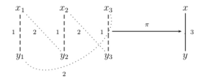
Figure 1. Example of a weighted covering graph
projection map \(\pi: V(Y) \to V(X)\) such that the following are true.
- 1. \(\pi\) is surjective and preserves adjacency.
- 2. For all \(x \in V(X)\) and \(y \in \pi^{-1}(x)\), the neighbors of y are mapped surjectively onto the neighbors of x. Thus, \(\pi \mid_{N(y)} \to N(x)\) is surjective for each y.
- 3. Let \(y \in V(Y)\) and \(x = \pi(y)\) in X. For each neighbor of x, \(n_x \in N(x)\),
\[\sum_{v \in \pi^{-1}(n_x)} w(y, v) = w(x, n_x) \tag{1}\]
Throughout the remainder of this paper, we refer to covering and base graphs as covers and bases, respectively.
In standard unweighted covering graph theory, Condition 3 above is replaced by requiring \(\pi\) to be an injection on each neighborhood of Y. In the context of weighted covers, Condition 3 requires that an edge weight in X equals the sum of the edge weights of its preimages with respect to \(\pi\) in Y. These two concepts are equivalent in the case of unweighted X and Y. Thus, the definition above generalizes the standard unweighted definitions.
In the case the edge weight function for X is integer valued, we may view Y as a cover for a multi-edged base X where each edge of X has weight 1. To define a cover for a graph with a multi-edged base it is necessary to extend the projection map \(\pi\) onto the edge sets as well. This in turn makes all of the arguments involving the projection map more technical and cumbersome. The edge weighted version allows for simpler arguments at the cost of a more subtle definition for Galois covers presented below.
Figure 1 is an example of a cover Y over a weighted base X. Vertices \(x,y \in V(X)\) with w(x,y)=3. The projection map \(\pi:V(Y)\to V(X)\) removes the subscripts of V(Y). The dashed edges in Y have weight 1. The dotted edges in Y have weight 2.
We present standard structural results which allow us to define subsets of V(Y) called sheets. We say a graph is finite if it has finitely many vertices.
Lemma 2.1. Let Y be a finite weighted cover of X with projection map \(\pi\). Let \((x_1, x_2)\) be an edge in E(X). Then \(|\pi^{-1}(x_1)| = |\pi^{-1}(x_2)|\).
Proof. Assume |π −1 (x1)| = k. From Condition 3, we have
\[\sum_{u \in \pi^{-1}(x_1)} \sum_{v \in \pi^{-1}(x_2)} w(u, v) = kw(x_1, x_2).\]
Beginning with the assumption that |π −1 (x2)| = m, we end with the same sum as the above equaling mw (x1, x2). Since w (x1, x2) > 0 as x1 ∼ x2, we have k = m.
Since we are assuming all of our graphs are connected, we can inductively follow a spanning tree in the base graph to argue all vertices in the base graph have the same number of preimages.
Theorem 2.1. Let Y be a finite weighted cover of X. Then |π −1 (x1)| = |π −1 (x2)| for all x1, x2 ∈ V (X).
The above theorem allows us to partition the vertices of Y into subsets or sheets consisting of unique preimages of all vertices in X under the projection map. More precisely, we partition V (Y ) into disjoint sheets S0, S1, . . . , Sd−1 where each Si contains exactly one element from each π −1 (x0), π−1 (x1), . . . , π−1 (xn−1) and V (X) = {x0, x1, . . . , xn−1}. This definition and the common cardinality of Theorem 2.1 gives us the number of sheets of a weighted cover.
For the purposes of analyzing the spectrum of the adjacency matrix of Y , we require more structure in the cover so that its adjacency matrix can be put in block diagonalized form. The structure will allow us to use a particular set of sheets to construct this block diagonalization form. Below we present the required structure on Y and this sheet construction. The structure will also give a canonical way to label the sheets. Following standard unweighted covering graph theory we define an appropriate notion of a weighted Galois covering graph.
To begin we define the automorphisms of Y over X in the context of weighted covers by requiring that the maps preserve edge weights as well.
Definition 2. Let Y be a weighted cover of X with projection map π. We say a function α : V (Y ) → V (Y ) is an automorphism of Y over X if:
- (1) α is a bijection that preserves both adjacency and non-adjacency,
- (2) For all y ∈ V (Y ), π(α(y)) = π(y). Thus, α preserves the projection map.
- (3) For all y1, y2 ∈ V (Y ), w (α (y1), α (y2)) = w (y1, y2). Thus, α preserves edge weights. Denote the set of automorphisms of Y over X as Aut(Y/X).
Definition 3. Let Y be a finite weighted cover of X where Y has d sheets. Then Y is a weighted Galois cover of X if there exists a subgroup G ⊂ Aut(Y/X) such that |G| = d and the nonidentity elements of G have no fixed vertices. We call G a Galois group of Y over X and denote such a subgroup as Gal(Y/X).
Some remarks are required about the above definition. In the case of unweighted covering graphs, it can be shown that non-identity automorphisms of the cover have no fixed vertices. Thus the size of Aut(Y/X) is bounded by the number of sheets of Y . In this case we say the cover is Galois if it has the maximal number of automorphisms as a cover of its base graph. However for weighted covering graphs, it is possible to see the appearance of "extra" automorphisms of the
cover. For example assume X is a single edge (u, v) with weight 3 and Y is the cover with vertices ui and vi for i = 0, 1, 2. The projection map π : Y → X maps ui to u and vi to v. Connect each ui to each vj by an edge of weight 1 so that Y is isomorphic to the complete bipartite graph K3,3. It is easy to see Aut(Y/X) = S3 × S3. However for purposes of analyzing the spectrum, we select a Galois subgroup such as Gal(Y/X) = {id, α1, α2} where αk (ui) = ui+k mod 3 and αk (vi) = vi+k mod 3 for k = 1, 2. In this case, there is a choice in the specific subgroup chosen for the Galois group but any such subgroup is sufficient to give extra structure to the adjacency matrix of the cover. We could equivalently require the Galois group to act freely on V (Y ) such that the quotient graph Y/Gal(Y/X) is isomorphic to X as in [14]. In general, determining necessary and sufficient conditions for the existence of these "extra" automorphisms of a weighted cover seems very subtle. We note that in the multi-edge version of these covering graphs the projection maps are required to be local isomorphisms at each vertex in the cover. Thus the number of automorphisms of the cover would be bounded by the number of sheets and the Galois definition would be more natural.
The importance of the definition of a weighted Galois cover is that it forces structure on the adjacency matrix AY of Y . It also gives a canonical way to label the sheets of the cover and forces a simpler block form for AY .
Let Y be a weighted d-sheeted Galois cover of X with Galois group G = Gal(Y/X), |G| = d, with projection map π : Y → X. Let X be composed of the vertices V (X) = {x0, x1, . . . , xm−1} and T an unweighted spanning tree of X. Define y (id) 0 to be any preimage of x0 under π. We label the sheets of Y by its Galois group elements. We begin by determining an identity sheet of Y . Since π is locally surjective we take a preimage Sid of T under π that contains y (id) 0 such that Sid ∼= T ignoring edge weights. We label the vertices in Sid as {y (id) i | π(y (id) i ) = xi , for each i = 0, 1, ..., m − 1}. The other sheets are now defined as the images of the identity sheet under the action of the Galois group. In particular, we let Sg = g (Sid) for g ∈ G. Extend the above notation by letting g y (id) i = y (g) i for each i and g. The definition of a weighted Galois cover now gives the following.
Lemma 2.2. Let Y be a weighted Galois cover of X with sheets Sg for g ∈ Gal(Y/X) defined as above. These sheets partition the vertices on Y . In particular, any two sheets are disjoint.
Proof. Assume g, h ∈ Gal(Y/X) and let vertex v ∈ Sg∩Sh. Since Sid contains a unique preimage of each vertex in X and both g and h preserve π, there is a vertex y (id) i such that g y (id) i = h y (id) i = v. Hence y (id) i = g −1 h y (id) i . Since g −1 ◦ h has a fixed vertex, it must be the identity. Hence g = h and Sg = Sh. The sheets cover V (Y ) by a simple counting argument and the lemma follows.
In order to simplify the adjacency matrix AY for Y , we set some notation. For each g ∈ G, define the m × m matrix A (g) with entries
\[\left(A\left(g\right)\right)_{i,j} = w\left(y_{i}^{\left(id\right)}, g\left(y_{j}^{\left(id\right)}\right)\right) = w\left(y_{i}^{\left(id\right)}, y_{j}^{\left(g\right)}\right)\]
where \(w \ge 0\) is the weight of the edge from \(y_i^{(id)}\) to \(g(y_j^{(id)})\). Loosely speaking, A(g) records the weights of the edges that originate at the vertices of sheet \(S_{id}\) and terminate at the vertices of the sheet \(S_g\). With this notation we can now describe the required structure in the adjacency matrix which motivates the definition of a weighted Galois cover.
Theorem 2.2. Assume as above that Y is a d-sheeted weighted Galois cover of X with Galois group \(G = \{g_0, g_1, \dots, g_{d-1}\}\) where \(g_0\) is the identity element of G. Then the adjacency matrix \(A_Y\) for Y can be written in the following form.
\[A_{Y} = \begin{pmatrix} A(g_{0}) & A(g_{1}) & A(g_{2}) & \dots & A(g_{d-1}) \\ A(g_{1}^{-1}) & A(g_{0}) & A(g_{1}^{-1}g_{2}) & \dots & A(g_{1}^{-1}g_{d-1}) \\ A(g_{2}^{-1}) & A(g_{2}^{-1}g_{1}) & A(g_{0}) & \dots & A(g_{2}^{-1}g_{d-1}) \\ \vdots & & & & \\ A(g_{d-1}^{-1}) & A(g_{d-1}^{-1}g_{1}) & A(g_{d-1}^{-1}g_{2}) & \dots & A(g_{0}) \end{pmatrix}\]
Proof. We label the vertices of Y in sheets \(S_q\) as above. For \(g_a, g_b \in G\) define the \(m \times m\) matrix
\[(A(g_a, g_b))_{i,j} = w\left(g_a\left(y_i^{(id)}\right), g_b\left(y_j^{(id)}\right)\right) = w\left(y_i^{(g_a)}, y_j^{(g_b)}\right).\]
Thus \(A(g_a, g_b)\) records the edges which contain one vertex of sheet \(S_{g_a}\) and one vertex of sheet \(S_{g_b}\). If we order the vertices of Y by its sheets, this matrix will represent the \((g_a, g_b)\) block of \(A_Y\). Now we note that since automorphisms preserve edge weights we have that
\[w\left(g_a\left(y_i^{(id)}\right), g_b\left(y_j^{(id)}\right)\right) = w\left(y_i^{(id)}, g_a^{-1}\left(g_b\left(y_j^{(id)}\right)\right)\right) = w\left(y_i^{(id)}, y_j^{(g_a^{-1}g_b)}\right).\]
Hence \(A(g_a, g_b) = A(g_a^{-1}g_b)\).
Example. Let \(X = K_{2,2}(3)\) be the complete bipartite graph with 2 vertices in each partition and every edge has weight 3. Let Y be the cover of X with Galois group \(G \approx \mathbb{Z}/5\mathbb{Z} = \{0, 1, 2, 3, 4\}\). Thus our theorem gives us
\[A_Y = \begin{pmatrix} A(0) & A(1) & A(2) & A(3) & A(4) \\ A(4) & A(0) & A(1) & A(2) & A(3) \\ A(3) & A(4) & A(0) & A(1) & A(2) \\ A(2) & A(3) & A(4) & A(0) & A(1) \\ A(1) & A(2) & A(3) & A(4) & A(0) \end{pmatrix}\]
where each A(i) is a \(4 \times 4\) matrix with non-negative entries and
\[\begin{pmatrix} 0 & 3 & 0 & 3 \\ 3 & 0 & 3 & 0 \\ 0 & 3 & 0 & 3 \\ 3 & 0 & 3 & 0 \end{pmatrix} = A(0) + A(1) + A(2) + A(3) + A(4).\]
The left hand side of the equality is the adjacency matrix \(A_X\) of X. We are free to define the entries of A(i) in a manner of our choice provided we satisfy the above sum. Since we are primarily concerned with constructing undirected graphs with no self-loops and no multiple edges, we can set
\[A(0) = \begin{pmatrix} 0 & 1 & 0 & 1 \\ 1 & 0 & 1 & 0 \\ 0 & 1 & 0 & 1 \\ 1 & 0 & 1 & 0 \end{pmatrix}, A(1) = \begin{pmatrix} 0 & 1 & 0 & 0 \\ 0 & 0 & 0 & 0 \\ 0 & 1 & 0 & 1 \\ 1 & 0 & 0 & 0 \end{pmatrix}\] and \[A(2) = \begin{pmatrix} 0 & 0 & 0 & 1 \\ 1 & 0 & 0 & 0 \\ 0 & 1 & 0 & 1 \\ 0 & 0 & 0 & 0 \end{pmatrix}\]
and \(A(3) = A(2)^{Tr}\), \(A(4) = A(1)^{Tr}\). The result is an undirected, connected, 6-regular graph Y realized as a weighted Galois cover of \(K_{2,2}\) with edge weights equal to 3 and Galois group \(\mathbb{Z}/5\mathbb{Z}\).
3. Ramanujan Graphs Constructed as Weighted Covers
In this section we construct finite families of Ramanujan graphs as Galois covers of bases with constant integral edge weights. We begin with a specific Ramanujan construction that allows for simple analysis of the resulting spectrum then argue that the construction can be generalized to produce more general Ramanujan graphs. We then consider various generalizations and consequences for further constructions. To begin we first record the definition of a regular Ramanujan graph. We define a simple graph as an undirected graph with no multiple edges and no self-loops.
Definition 4. Let X be a k-regular simple graph where Spec(X) is the set of eigenvalues of the adjacency matrix of X. Let \(\lambda = max\{|\mu| : \mu \in Spec(X), |\mu| \neq k\}\). Then X is a Ramanujan graph if \(\lambda \leq 2\sqrt{k-1}\).
As mentioned in the introduction, such graphs are optimal expander graphs and have many applications. Simple examples include complete graphs and complete bipartite graphs but not many other families of examples are known. See [11, 12] which present the best recent results. We give a new simple method for constructing Ramanujan graphs with fixed number of vertices and varying degree and note that the construction can be adjusted to fix the degree and vary the number of vertices.
Many of the graphs to follow have edge weights all with the same value. If a graph has edge weights all equal to a single value N then we say the graph has edge weights N.
3.1. Basic Construction
The outline of the basic construction of our Ramanujan graph is as follows. We fix the base graph to be bipartite graph \(K_{2,2}\) with edge weights \(N \in \mathbb{Z}^+\) and Galois group \(\mathbb{Z}/p\mathbb{Z}\) for prime p. We consider Galois covers of X with a particular form as a function of N. These specializations give the adjacency matrix for Y a simple form. We then use a block diagonalization theorem to block diagonalize the adjacency matrix of Y. The Gershgorin Circle Theorem is used to evaluate
the entries of these blocks. The result is a bound on the eigenvalues of the blocks as a function of N. Finally the values of N are chosen to ensure the graphs satisfy the Ramanujan bound.
We let \(X = K_{2,2}(N)\) denote the bipartite graph with edge weights N and partition its vertices as \(\{x_0, x_2\}\) and \(\{x_1, x_3\}\). Hence the adjacency matrix of X is
\[A_X = \left(\begin{array}{cccc} 0 & N & 0 & N \\ N & 0 & N & 0 \\ 0 & N & 0 & N \\ N & 0 & N & 0 \end{array}\right).\]
Note that since the eigenvalues of \(K_{2,2}\) are \(\pm 2\) and 0 with multiplicity 2, the eigenvalues of \(K_{2,2}(N)\) are \(\pm 2N\) and 0 with multiplicity 2.
For simplicity we fix a prime p > N and consider a Galois cover Y of X with Galois group \(G(Y/X) = \mathbb{Z}/p\mathbb{Z}\). We define a particular cover Y whose adjacency matrix \(A_Y\) has the following form. For each \(k \in Gal(Y/X) \approx \mathbb{Z}/p\mathbb{Z}\), define the entries of matrix A(k) as follows.
\[A(k) = \begin{pmatrix} 0 & a_{0,1}^{(k)} & 0 & a_{0,3}^{(k)} \\ a_{1,0}^{(k)} & 0 & a_{1,2}^{(k)} & 0 \\ 0 & a_{2,1}^{(k)} & 0 & a_{2,3}^{(k)} \\ a_{3,0}^{(k)} & 0 & a_{3,2}^{(k)} & 0 \end{pmatrix}\]
where
\[\text{[rumus tidak dapat ditampilkan dengan baik — lihat PDF asli]}\]
These matrices compose \(A_Y\) as described in Theorem 2.2. Define B as the adjacency matrix for \(K_{2,2}\), C the matrix whose upper triangular part is the same as B but with 0 below its diagonal, \(D = C^t\), and \(\mathbb O\) the \(4 \times 4\) zero matrix. Then the first block row of \(A_Y\) has the form \((B \ C \ C \ C \ \dots \ \mathbb O \ \mathbb O \ \dots \ D \ D \ D \ \dots)\) if N < p/2 and \((B \ C \ C \ C \ \dots \ B \ B \ \dots \ D \ D \ D \ \dots)\) otherwise. Note that Y is an undirected graph with edge weights 1. Also Y has no self-loops and no multiple edges where the degree of each vertex is 2N. Since the Galois group is \(\mathbb Z/p\mathbb Z\), we can write \((A_Y)_{i,j}\) as a \(4 \times 4\) block where \((A_Y)_{i,i} = B\) and \((A_Y)_{i,j} = (A_Y)_{0,j-i} = A(j-i)\) for \(i \neq j\) and i,j taken modulo p.
We now show that for N large enough, Y is a Ramanujan graph.
Theorem 3.1. Let \(X = K_{2,2}(N)\) be the bipartite graph with edge weights \(N \in \mathbb{Z}^+\), p prime with p > N, and Y the Galois cover of base X constructed above. Let
\[\alpha_p = \frac{p^2}{p^2 - \pi^2/3!}.\]
Then Y is a Ramanujan graph for all N such that
\[p + \frac{1 - \sqrt{(2p-1)\alpha_p^2 + 1}}{\alpha_p^2} < N \le p.\] (2)
Note that \(\alpha_p > 0\) for all primes p. Also \(\alpha_p \to 1\) as \(p \to \infty\). Thus asymptotically we need N greater than \(p+1-\sqrt{2p}\). Note that in the construction we are taking p as fixed and letting N vary. However we can fix N and let p vary to satisfy the bound in the theorem to get families of Ramanujan graphs with fixed degree 2N. Although each family will be finite in size, the size of the families goes to infinity as N increases to infinity.
To prove Theorem 3.1, we use a generalization of the block diagonalization theorem in [13]. The proof of the theorem relies on decomposing the right regular representation into irreducible components. The entries of the adjacency matrix play no role in the theorem. Thus the proof given in [13] can be generalized to show the following result.
Definition 5. Let \(A = (a_{i,j})\) and B be matrices. Then the tensor product of A and B, \(A \otimes B\), is
\[A \otimes B = \left(\begin{array}{ccc} a_{1,1}B & a_{1,2}B & \cdots \\ a_{2,1}B & a_{2,2}B & \cdots \\ \vdots & \vdots & \ddots \end{array}\right).\]
Theorem 3.2. [13] Let Y be a d-sheeted weighted Galois cover of X with \(Gal(Y/X) = \{g_1, g_2, \dots, g_d\}\). The adjacency matrix for Y can be block diagonalized into blocks of the form
\[M_{\pi} = \sum_{g \in Gal(Y/X)} d_{\pi}\pi(g) \otimes A(g), \tag{3}\]
where \(\pi\) runs through the irreducible representations of Gal(Y/X), \(d_{\pi}\) is the degree of the representation \(\pi\), and the matrices A(q) described in Theorem 2.2.
We are ready to prove Theorem 3.1.
Proof. (to Theorem 3.1) In the construction we have \(Gal(Y/X) = \mathbb{Z}/p\mathbb{Z}\). Hence all of the representations are the one-dimensional characters \(\chi_k(g) = exp\left(2\pi i g k/p\right)\) for \(k \mod p\). Applying our block diagonalization theorem above with \(M_{\chi_k} = M_k\) denoting the k-th \(4 \times 4\) diagonal block, we have
\[M_k = \sum_{j \bmod p} \chi_k(j) A(j).\]
Due to the way we created Y, each \(M_k\) has the form
\[M_k = \begin{pmatrix} 0 & a_k & 0 & a_k \\ b_k & 0 & a_k & 0 \\ 0 & b_k & 0 & a_k \\ b_k & 0 & b_k & 0, \end{pmatrix}\]
where \(a_k\) and \(b_k\) are sums of roots of unity. We see that \(a_0 = b_0 = N\) and in general, the \(a_k\) and \(b_k\) have the form
\[a_k = \sum_{j=0}^{N-1} exp(2\pi i j k/p), \ b_k = \sum_{j=0}^{N-1} exp(-2\pi i j k/p),\]
for \(k \mod p\). There is a formula for such sums. Thus
\[a_k = \frac{\sin(\pi N k/p)}{\sin(\pi k/p)} e^{\frac{\pi i(N-1)k}{p}}, \ b_k = -\bar{a}_k,\]
since sin(-x) = -sin(x).
We look for conditions on N in order that \(A_Y\) satisfies the Ramanujan bound. In particular if \(\lambda\) is an eigenvalue of \(A_Y\) with \(\lambda \neq \pm 2N\) we require \(|\lambda| \leq 2\sqrt{2N-1}\). Note that \(M_0 = A_X\) which has eigenvalues \(\pm 2N\) and 0. For the eigenvalues of the other \(M_k\)s, we use the Gershgorin Circle Theorem which says that the eigenvalues of \(M_k\) are bounded by \(2|a_k| = 2|b_k|\). Thus we seek to bound \(|a_k|\). In particular we seek conditions on N such that \(2\left|\frac{\sin(\pi N k/p)}{\sin(\pi k/p)}\right| \leq 2\sqrt{2N-1}\) for all \(k=1,2,\ldots,p-1\).
We claim that if the inequality is true for k=1 then it is true for all other k. In fact we prove a more general result about sums of distinct p-th roots of unity and provide an upper bound on the absolute value of the sum of r distinct p-th roots of unity.
Lemma 3.1. Let p be a positive integer and \(S_{r,p}\) a sum of any r distinct p-th roots of unity where 0 < r < p. Then
\[|S_{r,p}| \le \left| \sum_{j=0}^{r-1} e^{2\pi i j/p} \right|.\]
More generally the absolute value of \(S_{r,p}\) is bounded by the absolute value of the sum of any r consecutive p-th roots of unity.
Proof. The lemma follows from noting the length of a sum of vectors is the sum of their projections onto the resulting sum. More precisely, assume \(z_1, z_2, ..., z_k\) are the roots of unity where we denote each \(z_j = e^{i\theta_j}\). Let \(v = \sum_i z_j = re^{i\phi}\) with r > 0. Then
\[|v|^2 = v \cdot v = \left(\sum_{j=1}^k z_j\right) re^{-i\phi} = r^2.\]
Hence we have
\[r = \sum_{j=1}^{k} e^{i(\theta_j - \phi)}.\]
Since r is real the sine terms vanish and
\[r = \sum_{j=1}^{k} \cos(\theta_j - \phi).\]
Thus to maximize r we need to maximize each of the individual cosine terms by taking the roots of unity as close as possible to the resultant vector and the result follows.
We note that the above argument can easily be generalized to a finite number of repetitions in the sum. In particular if we allow up to t repeating p-th roots of unity in our sum of r roots, the absolute value is bounded by t times the absolute value of the sum of the first \(\lceil \frac{r}{t} \rceil p\)-th roots of unity. This result would allow us to extend these techniques to more general finite abelian Galois groups.
Returning to the proof of Theorem 3.1, Lemma 3.1 allows us to assume k=1. Thus we want a bound on
\[\left| \frac{\sin(\pi N/p)}{\sin(\pi/p)} \right|.\]
We note \(sin\left(x\right) < x\) for all x > 0 and \(sin\left(\pi/p\right) > \frac{\pi}{p} - \frac{\pi^3}{p^3 3!}\). Further \(|sin\left(\pi x\right)| = |sin\left(\pi\left(1x\right)\right)|\). Hence
\[\left|\frac{\sin\left(\pi N/p\right)}{\sin(\pi/p)}\right| = \left|\frac{\sin\left(\pi\left(p-N\right)/p\right)}{\sin(\pi/p)}\right| < \frac{\pi\left(p-N\right)/p}{\pi/p - \pi^3/\left(p^3 3!\right)} = \frac{\left(p-N\right)p^2}{p^2 - \pi^2/3!}.\]
Let \(\alpha_p = \frac{p^2}{p^2 - \pi^2/3!}\). Thus the Ramanujan bound becomes
\[(p-N)\,\alpha_p \le \sqrt{2N-1}.\]
Solving the inequality we get the bound on N,
\[N \ge p + \frac{1 - \sqrt{\left(2p - 1\right)\alpha_p^2 + 1}}{\alpha_p^2}.\]
Letting p go to infinity and thus \(\alpha_p \to 1\), we have
\[N \ge p + 1 - \sqrt{2p}.\]
Hence for all \(N \geq p + \frac{1 - \sqrt{(2p-1)\alpha_p^2 + 1}}{\alpha_p^2}\), the Gershgorin radii of the blocks corresponding to the non-trivial characters are less than the Ramanujan bound. Hence the construction yields a Ramanujan graph. Note that \(N \leq p\) to avoid edge weights other than 0 and 1 in the adjacency matrix of the cover.
3.2. Numerical Results
We present computational data to illustrate the lower bound of Theorem 3.1. For fixed p, let \(N_T\) be our theoretical lower bound on N,
\[N_T = p + \frac{1 - \sqrt{(2p-1)\,\alpha_p^2 + 1}}{\alpha_p^2},\]
where \(\alpha_p=p^2/\left(p^2-\pi^2/3!\right)\). For each N, define \(\lambda_2\) as the second largest eigenvalue of the resulting cover and the Ramanujan bound as \(RAM=2\sqrt{2N-1}\). Let GERSH be the Gershgorin bound on \(\lambda_2\) which is twice the bound in Lemma 3.1.
| N | 85 | 86 | 87 | 88 | 89 | 90 |
|---|---|---|---|---|---|---|
| \(\lambda_2\) | 29.63 | 28.03 | 26.39 | 24.70 | 22.97 | 21.20 |
| RAM | 26 | 26.15 | 26.30 | 26.45 | 26.60 | 26.75 |
| GERSH | 30.70 | 28.93 | 27.13 | 25.30 | 23.45 | 21.58 |
Figure 2. Computational data for p = 101
| N | 1172 | 1173 | 1174 | 1175 | 1176 | 1177 |
|---|---|---|---|---|---|---|
| \(\lambda_2\) | 101.48 | 99.51 | 97.54 | 95.56 | 93.59 | 91.61 |
| RAM | 96.80 | 96.85 | 96.89 | 96.93 | 96.97 | 97.01 |
| GERSH | 101.71 | 99.73 | 97.74 | 95.76 | 93.77 | 91.79 |
Figure 3. Computational data for p = 1223
For p=101, we compute \(N_T=87.71\). Table 2 presents \(\lambda_2\), RAM, and GERSH for N near \(N_T\).
For p=1223, we compute \(N_T=1174.52\). Table 3.2 presents \(\lambda_2\), RAM, and GERSH for N near \(N_T\).
Note that the data shows our bounds on N appearing in Theorem 3.1 are sharp for p=101 and 1223. We also note that the bounds of \(\lambda_2\) arising from the Gershgorin bound appear quite sharp also.
3.3. Generalizing the Construction
A question to ask is: To what extent can the above calculations be generalized to produce more Ramanujan graphs as weighted Galois covers? Although our cover construction is special it is possible to construct other families of Ramanujan graphs. In particular we show that given a Galois cover Y of \(K_{2,2}(N)\) with N as in the above theorem and Galois group \(\mathbb{Z}/p\mathbb{Z}\), Y is also a Ramanujan graph.
Theorem 3.3. Let Y be a simple weighted Galois cover with edge weights 1 over base \(X = K_{2,2}(N)\) where \(N \geq p + \frac{1 - \sqrt{(2p-1)\alpha_p^2 + 1}}{\alpha_p^2}\), and \(Gal(Y/X) = \mathbb{Z}/p\mathbb{Z}\) with p prime. Then Y is a Ramanujan graph.
Proof. Suppose Y is a weighted Galois cover of \(X = K_{2,2}(N)\) and \(Gal(Y/X) = \mathbb{Z}/p\mathbb{Z}\) for prime p, whose edge weights are all 1. As above we select one pre-image of every vertex in the base graph as our initial sheet \(S_{id}\). Define the other sheets S(g) as the images of \(S_{id}\) under the action of \(g \in Gal(Y/X)\). Since Y is a Galois cover, by Theorem 2.2 we can write the adjacency matrix of Y in blocks A(g). Since all of the non-zero edge weights of Y are Y, the entries of each of the Y matrices are in Y using the block diagonalization theorem we have that Y can be block diagonalized into blocks of the form
\[M_{\chi} = \sum_{g \in Gal(Y/X)} \chi(g) \otimes A(g)\]
where χ is a character modulo p. As above M0 = AX and thus has eigenvalues 0, ±2N. For each of the non-trivial characters χ, the entries of Mχ are either zero or a sum of N distinct p-th roots of unity. Thus by Lemma 3.1 each of the non-zero entries is bounded by the norm of the sum of the first N p-th roots of unity. Hence the Gershgorin bounds arising for Y are bounded by those arising in our construction above. Thus the same lower bound on N ensures that Y is a Ramanujan graph.
Note that generalizing the techniques from standard unweighted covering graph theory found in [1, 5, 6], we can explicitly write down all of these graphs.
4. Further Generalizations and Questions
First note that the Galois groups chosen above are done mostly for simplicity. We could look at more general finite abelian groups without added complications. The main difference is the bounds arising from Lemma 3.1 change since we may not have a sum of distinct roots of unity. More general Galois groups make calculating the blocks for the adjacency matrix of the cover a more difficult task.
Begin with a d-regular base graph X with edge weights 1. Let X(N) be the weighted version of X where all of the edge weights are N. Let Y be a graph with edge weights 1 where Y is a weighted Galois cover of X(N). Regardless of the Galois group, the block diagonal of AY corresponding to the trivial representation is AX(N) . Thus Spec(X(N)) = N ∗ Spec(X) ⊆ Spec(Y ). Let λX(N) and λY be second largest eigenvalues in absolute value of AX(N) and AY , respectively. Then λY ≥ λX(N) = NλX. In order for Y to be a Ramanujan graph we require
\[N\lambda_X \le \lambda_Y \le 2\sqrt{dN - 1} \tag{4}\]
or
\[\lambda_X \le 2\sqrt{\frac{d}{N} - \frac{1}{N^2}}. (5)\]
Thus X must satisfy an even stronger condition than the Ramanujan condition on Y if Y is to be a Ramanujan graph. The bound above forces conditions on the base graph and the weights of its edges. In particular we have the following.
Theorem 4.1. Let Y be a weighted Galois cover of the weighted graph X(N) for some connected d-regular graph X and edge weight N ∈ Z +, such that Y is a Ramanujan graph. Then
\[\lambda_X \le 2\frac{\sqrt{dN-1}}{N} = 2\sqrt{\frac{d}{N} - \frac{1}{N^2}}.\tag{6}\]
If λX 6= 0 then
\[N \le \frac{2d + 2\sqrt{d^2 - \lambda_X^2}}{\lambda_X^2}. (7)\]
This explains the choice of the complete bipartite graph as a basis for our construction since λK2,2 = 0 and thus λK2,2(N) = 0. Since the complete regular bipartite graphs all have λKm,m = 0, they represent a family of potential base graphs for Ramanujan graphs Y . If we let our base graph be X(N) = Km,m(N), we get the following general theorem.
Theorem 4.2. Let X = Km,m with edge weights N ∈ Z +, p prime with p > N, and αp as above. Let Y be a Galois cover of X constructed as in Theorem 3.1 or 3.3. Then Y is a Ramanujan graph if
\[p + \frac{2 - 2\sqrt{(mp - 1)\alpha_p^2 + \frac{4}{m^2}}}{m\alpha_p^2} \le N \le p.\] (8)
This allows us to create families of Ramanujan graphs with 2mp vertices for a prime p and degrees ranging over a shorter range.
Another reasonable choice of base graph is the complete graphs Km since λKm = 1. Applying Theorem 4.1 gives the following.
Corollary 4.1. Let Y be a graph with weighted edges 1 and Y a Galois cover of X = Km(N). If Y is a Ramanujan graph then
\[N \le 2(m-1) + 2\sqrt{((m-1)^2 - 1)}.\]
4.1. Further Questions
From a constructivist point of view, Theorem 4.1 gives explicit conditions for potential weighted base graphs and potential weights from which to try and construct Ramanujan covers. One direction for future study is to try and generalize the constructions given here to other families of base graphs. Another direction is to vary the Galois group. We outlined above how to generalize the argument above to finite abelian Galois groups but it would be interesting to understand the nonabelian case as well. The specific construction above was chosen primarily for ease of calculation. It would be interesting to investigate more clever ways of assigning the edges between the sheets to try and minimize the resulting character sums. Another possible construction involves base graphs with non-constant edge weight. Finally, zeta functions and L-functions have been well studied in the case of weighted graphs and as covering graphs. See [2, 8, 14, 15, 16, 17]. A natural question to ask is how properties of the natural zeta and L-functions arising from these weighted covering graphs compare to those in the above cases.
Acknowledgement
The authors thank the referee for comments that helped the clarity of this paper.
References
[1] Y. Bilu and N. Linial, Lifts, Discrepancy and Nearly Optimal Spectral Gap, Combinatorica 26 (5) (2006), 495–519.
- [2] Y-B. Choi, J-H Kwak, Y-S Park and I. Sato, Bartholdi Zeta and L-functions of Weighted Digraphs Their Coverings and Products, Advances in Math. 213 (2007), 865–886.
- [3] S. Corry, Harmonic Galois theory for Finite Graphs, in "Galois-Teichmuller Theory and ¨ Arithmetic Geometry", Advanced Studies in Pure Math. 63 (2012), 121–140.
- [4] A. Deng, I. Sato and Y. Wu, Homomorphisms, Representations, and Characteristic Polynomials in Digraphs, Linear Algebra Appl. 423 (2007), 386–407.
- [5] J. Gross and T. Tucker, Generating All Graph Coverings by Permutation Voltage Assignments, Discrete Math. 18 (1977), 273–283.
- [6] J. Gross and T. Tucker, Topological Graph Theory, Wiley, (1987).
- [7] S. Hoory, N. Linial and A. Widgerson, Expander Graphs and Their Applications, Bull. Amer. Math. Soc. 34 (4) (2006), 439–561.
- [8] M. Horton, H. Stark and A. Terras, Zeta Functions of Weighted Graphs and Covering Graphs, in Analysis on Graphs, Proc. Symp. Pure Math. 77 (2008).
- [9] T. Kaufman and A. Lubotzky, Edge Transitive Ramanujan Graphs and Symmetric LPDC Good Codes, STOC '12, (2012), 359–366.
- [10] A. Lubotzky, R. Phillips and P. Sarnak, Ramanujan Graphs, Combinatorica 8(3) (1988), 261– 277.
- [11] A. Marcus, D. Spielman and N. Srivastava, Interlacing Families I: Bipartite Ramanujan Graphs of All Degrees, Ann. of Math. 182 (1) (2015), 307–325.
- [12] A. Marcus, D. Spielman and N. Srivastava, Interlacing Families IV: Bipartite Ramanujan Graphs of All Sizes, FOCS (2015).
- [13] M. Minei and H. Skogman, Block Diagonalization Method for the Covering Graph, Ars Combin. 92 (2009), 321–352.
- [14] I. Sato, Weighted Zeta Functions of Graph Coverings, Electron. J. Combin. 13 (2006)
- [15] H. Stark and A. Terras, Zeta functions of Finite Graphs and Coverings, Adv. Math. 121 (1996), 124–165.
- [16] H. Stark and A. Terras, Zeta functions of Finite Graphs and Coverings, Pt. II, Adv. Math. 5 (2000), 132–195.
- [17] H. Stark and A. Terras, Zeta functions of Finite Graphs and Coverings, Pt. III, Adv. Math. 208 (1) (2007), 467–489.
- [18] A. Valette, Graphes de Ramanujan et Applications, Asterisque 245 (1997), 247–276.