Fendy Septyanto, Kiki A. Sugeng

Departments of Mathematics, Faculty of Mathematics and Natural Sciences, Universitas Indonesia, Depok - Indonesia

fendy.septyanto41@sci.ui.ac.id, kiki@sci.ui.ac.id

Let G be a graph with an edge k-coloring γ : E(G) → {1, . . . , k} (not necessarily proper). A path is called a rainbow path if all of its edges have different colors. The map γ is called a rainbow coloring if any two vertices can be connected by a rainbow path. The map γ is called a strong rainbow coloring if any two vertices can be connected by a rainbow geodesic. The smallest k for which there is a rainbow k-coloring (resp. strong rainbow k-coloring) on G is called the rainbow connection number (resp. strong rainbow connection number) of G, denoted rc(G) (resp. src(G)). In this paper we generalize the notion of "color codes" that was originally used by Chartrand et al. in their study of the rc and src of complete bipartite graphs, so that it now applies to any connected graph. Using color codes, we prove a new class of lower bounds depending on the existence of sets with common neighbours. Tight examples are discussed, involving the amalgamation of complete graphs, generalized wheel graphs, and a special class of sequential join of graphs.

Keywords: clique, color code, common neighborhood, independence, rainbow connection

Mathematics Subject Classification : 05C15

DOI: 10.5614/ejgta.2018.6.2.14

1. Introduction

In 2008, Chartrand et al. introduced rainbow colorings, as a way to strengthen connectedness. A coloring on a graph G refers to any map γ : E(G) → {1, . . . , k}, which is also called edge-

Received: 5 October 2017, Revised: 19 August 2018, Accepted: 17 September 2018.

coloring or k-coloring. We write x = y to say \(xy \in E(G)\) and \(\gamma(xy) = i\). A path

\[v_1^{c_1} v_2^{c_2} \cdots v_n^{c_{n-1}} v_n \tag{1.1}\]

with color sequence \(c_1, c_2, \dots, c_{n-1}\) is said to be a rainbow path if all of its edges have different colors. A coloring is called a rainbow coloring if any two vertices can be connected by a rainbow path. A trivial way to produce a rainbow coloring on any connected graph is using |E(G)| colors to give each individual edge its own color. This may not be efficient, e.g. two colors are enough to rainbow-color \(C_4\) (put 1 and 2 alternately). The smallest k for which there is a rainbow k-coloring on G is called the rainbow connection number of G, denoted by rc(G).

These notions can be developed further by considering the notion of a geodesic, which is a shortest path between two vertices x, y in a graph G. The distance \(d_G(x, y)\) is defined as the length of any such shortest path. The diameter of G, denoted by diam(G), is defined as the largest distance between pairs of vertices of G. A coloring is called a strong rainbow coloring if any two vertices can be connected by a rainbow geodesic. The smallest k for which there is a strong rainbow k-coloring on G is called the strong rainbow connection number of G, denoted by src(G).

Chartrand et al. [1] noted the following chain,

\[diam(G) \le rc(G) \le src(G) \le |E(G)|. \tag{1.2}\]

Some equality cases are known. The complete graphs are the only graphs whose rc and src are equal to 1, and trees are the only graphs whose rc and src are equal to the number of edges in those graphs (see [1]). However, it remains open to characterize when rc(G) = diam(G).

Li and Sun [5] tightened the upper bound to \(src(G) \leq |E(G)| - 2t\), where t is the number of edge-disjoint triangles. Schiermeyer [7] observed a different lower bound \(rc(G) \geq n_1(G)\), where \(n_1\) is the number of vertices of degree one. The reader is referred to [6] for a more detailed survey.

In this paper, we prove some lower bounds based on the presence of sets with common neighbours. For a non-empty \(Q \subseteq V(G)\), its common neighborhood is denoted

\[CN(Q) = \bigcap_{v \in Q} N(v) \tag{1.3}\]

A new graph \(Q^*\) (called the CN-graph of Q) is defined with \(V(Q^*) = Q\) such that \(v, w \in Q\) are adjacent in \(Q^*\) if and only if they are already adjacent in G, or \(CN(v, w) \neq CN(Q)\). In Section 2.1 we prove that if \(CN(Q) \neq \emptyset\) then

\[src(G) \ge \max \left\{ \beta_0(Q^*), \frac{|Q|}{\omega(Q^*)} \right\}^{\frac{1}{|CN(Q)|}}\] \[(1.4)\]

where \(\beta_0\) is the vertex-independence number, and \(\omega\) is the clique number. These parameters are described e.g. in [4]. We also prove a version of (1.4) for multiple sets. In Section 2.2 we prove similar bounds for rc. In Section 2.3 we discuss some miscellaneous bounds that will be useful in our discussion of tight examples involving the amalgamation of complete graphs, generalized wheel graphs, and a class of sequential join.

We use color codes. This notion was used in [1] as a tool to study the rc and src of complete bipartite graphs. Now we adapt it to any connected graph. Given a coloring γ : E(G) → {1, . . . , k} (not necessarily rainbow) and a non-empty set Q ⊆ V (G) with non-empty common neighborhood CN(Q) = {t1, . . . , tb}, we define the color code of a vertex v ∈ Q as follows,

\[code(v) = (\gamma(vt_1), \gamma(vt_2), \cdots, \gamma(vt_b)). \tag{1.5}\]

The tuple code(v) depends on the set Q that we consider v a member of, as illustrated in Figure 1.

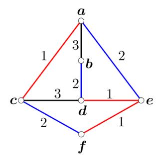
Figure 1. If we consider a ∈ {a, d}, code(a) is a 3-tuple. It is a 2-tuple if we consider a ∈ {a, d, f}.

To avoid ambiguity, we also refer to the tuple (γ(vt1), γ(vt2), · · · , γ(vtb)) as the code of v with respect to {t1, . . . , tb}. Let code(Q) = {code(v)|v ∈ Q}. Since every code is a b-tuple, we have

\[|code(Q)| \le k^b. \tag{1.6}\]

Lemma 1.1. Let γ be a coloring on G, and Q ⊆ V (G) with CN(Q) 6= ∅. Then there is a rainbow geodesic between two non-adjacent vertices in Q^∗ if and only if their color codes are different.

Proof. Let v, w ∈ Q but vw 6∈ E(Q^∗ ). Any v−w geodesic has the form v−t−w with t ∈ CN(Q). So there is a rainbow v−w geodesic if and only if there is a t ∈ CN(Q) with γ(vt) 6= γ(wt).

A set is called co-neighboring if any two of its vertices have precisely the same (non-empty) neighborhood. An independent set has any two of its vertices non-adjacent.

Lemma 1.2. Let γ be a coloring on G, Q ⊆ V (G) co-neighboring, and CN(Q) independent. If v, w ∈ Q and code(v) = code(w), then the length of any rainbow path between them is at least 4.

Proof. Since Q is co-neighboring, vw 6∈ E(G) and N(v) = N(w) = CN(Q). So vw 6∈ E(Q^∗ ). By Lemma 1.1 there are no rainbow v−w geodesics. Let L : v−x− · · · −y−w be a rainbow path with x ∈ N(v) and y ∈ N(w). Then x, y ∈ CN(Q) and x 6= y (since L is not geodesic). So, the length of L is at least 2 + dG(x, y) ≥ 4 because x, y are non-adjacent.

Lemma 1.3. Let γ be a coloring on G, and Q ⊆ V (G) with CN(Q) 6= ∅. If

\[|code(Q)| < \max\left\{\beta_0(Q^*), \frac{|Q|}{\omega(Q^*)}\right\},\tag{1.7}\]

then there are non-adjacent vertices in Q^∗ with the same color code.

Proof. Let b = |CN(Q)|. If |code(Q)| < β0(Q^∗ ), then let X ⊆ Q be an independent set in Q^∗ with |X| = β0(Q^∗ ); since |X| > |code(Q)|, some two v, w ∈ X have the same code.

If |code(Q)| < |Q| ω(Q∗) , then |code(Q)|ω(Q^∗ ) < |Q| so at least ω(Q^∗ ) + 1 vertices in Q have the same code; if X is a set of such vertices, then some v, w ∈ X are non-adjacent in Q^∗ .

Later we deal with multiple subsets. The problem is how to compare the codes in different subsets. Let us call two disjoint sets Q1, Q² ⊆ V (G) CN-bridged if for every v ∈ Q¹ and w ∈ Q² we have v and w non-adjacent in G, and any geodesic between them has the form v−x− · · · −y−w with x ∈ CN(Q1) and y ∈ CN(Q2). A diagonal tuple has the form (i, i, . . . , i).

Lemma 1.4. Let Q1, . . . , Q^p ⊆ V (G) with p ≥ 2 and |CN(Qi)| = b for all i ∈ {1, . . . , p}, and let γ be a k-coloring on G. Suppose there is a natural number r that satisfies the following condition,

\[r \le k \le \sqrt[b]{\frac{1}{p} \left(r - 1 + \sum_{i=1}^{p} \max\left\{\beta_0(Q_i^*), \frac{|Q_i|}{\omega(Q_i^*)}\right\}\right)}.\] (1.8)

Then one of the following must hold:

• (1) For some i ∈ {1, . . . , p}, there are non-adjacent vertices in Q^{∗ i} with the same code.
• (2) For some i, j ∈ {1, . . . , p} with i 6= j, there is a diagonal tuple in code(Qi) ∩ code(Q^j ).

Proof. Suppose (1) fails to hold. Let A and B be the set of diagonal and non-diagonal b-tuples of numbers from {1, . . . , k}, respectively. Then |A| = k and |B| = k ^b − k. We need to show code(Qi) ∩ code(Q^j ) ∩ A 6= ∅ for some i 6= j. Assuming otherwise, for all i 6= j we have

\[0 = |code(Q_i) \cap code(Q_j) \cap A| \geq |code(Q_i) \cap A| + |code(Q_i) \cap A| - |A|\]
\[\geq |code(Q_i)| - |B| + |code(Q_j)| - |B| - |A|\]
\[= |code(Q_i)| + |code(Q_j)| - 2k^b + k\]

so 2k ^b − k ≥ |code(Qi)| + |code(Q^j )|. Summed up, p 2 (2k ^b − k) ≥ (p − 1)P^{p i}=1 |code(Qi)|. Hence

\[k^b - \frac{1}{p} \sum_{i=1}^p |code(Q_i)| \ge \frac{k}{2} \ge \frac{r}{2}.\] (1.9)

Since (1) fails, we have ^|code(Qi)| ≥ max β0(Q^∗ i ), |Qi| ω(Q^∗ i ) for 1 ≤ i ≤ p by Lemma 1.3. So

\[\frac{r}{2} \le k^b - \frac{1}{p} \sum_{i=1}^p |code(Q_i)| \le k^b - \frac{1}{p} \sum_{i=1}^p \max \left\{ \beta_0(Q_i^*), \frac{|Q_i|}{\omega(Q_i^*)} \right\} \le \frac{r-1}{p}\] (1.10)

where the rightmost inequality in (1.10) follows from the rightmost inequality in the hypothesis (1.8). Since p ≥ 2, we get ^{r 2} ≤ r−1 ^p ≤ r−1 2 , a contradiction.

2. Main Results

2.1. Lower bounds for src

Theorem 2.1. Let G be a connected graph and \(Q \subseteq V(G)\) with \(CN(Q) \neq \emptyset\). Then

\[src(G) \ge \max \left\{ \beta_0(Q^*), \frac{|Q|}{\omega(Q^*)} \right\}^{\frac{1}{|CN(Q)|}}.\] (2.1)

Proof. Let b = |CN(Q)|. Suppose \(src(G) \le k\), where \(k = \left\lceil \sqrt[b]{\max\left\{\beta_0(Q^*), \frac{|Q|}{\omega(Q^*)}\right\}} \right\rceil - 1\) Under a strong rainbow k-coloring on G, we have \(|code(Q)| \le k^b < \max\left\{\beta_0(Q^*), \frac{|Q|}{\omega(Q^*)}\right\}\). So Lemma 1.3 applies, and we get a contradiction with Lemma 1.1.

If we have several subsets \(Q_1, \ldots, Q_p \subseteq V(G)\), then an application of Theorem 2.1 to each individual set gives p lower bounds, which can be averaged to

\[src(G) \ge \frac{1}{p} \sum_{i=1}^{p} \sqrt[b]{\max\left\{\beta_0(Q_i^*), \frac{|Q_i|}{\omega(Q_i^*)}\right\}}.\] (2.2)

The following is a better bound that incorporates all the subsets simultaneously, under the additional assumption that the sets are pairwise CN-bridged. Moreover, the bound can also make use of a previously known lower bound for src and possibly improve it to a sharper bound.

Theorem 2.2. Let G be a connected graph, \(p \ge 2\), and \(Q_1, \ldots, Q_p \subseteq V(G)\) be pairwise CN-bridged sets with \(|CN(Q_i)| = b > 0\) for \(1 \le i \le p\). If \(src(G) \ge r\) for some \(r \in \mathbb{N}\), then

\[src(G) \ge 1 + \left| \sqrt[b]{\frac{1}{p} \left( r - 1 + \sum_{i=1}^{p} \max \left\{ \beta_0(Q_i^*), \frac{|Q_i|}{\omega(Q_i^*)} \right\} \right)} \right|.\] (2.3)

Proof. Suppose \(src(G) \leq k\), where k is the right hand side minus 1. Let \(\gamma\) be a strong rainbow k-coloring on G. Note that (1.8) holds, so one of the options (1) or (2) in Lemma 1.4 holds. If (1) holds, Lemma 1.1 is contradicted. So (2) holds. Let \(v \in Q_i\) and \(w \in Q_j\) have the same diagonal tuple as their code. By CN-bridging, any v-w geodesic has the form \(v-x-\cdots-y-w\) with \(x \in CN(Q_i)\) and \(y \in CN(Q_j)\). But \(\gamma(vx) = \gamma(wy)\), so this geodesic is not rainbow. \(\square\)

Remark 2.1. Even if we start with the trivial estimate r=1, this is already stronger than the average bound (2.2), due to Jensen's inequality for the concave function \(f(x) = \sqrt[b]{x}\) on \(x \ge 0\) and the fact that \(1 + \lfloor x \rfloor > x\).

2.2. Lower bounds for rc

We consider analogous version of the previous bounds for rainbow connection number.

Theorem 2.3. Let G be a connected graph and \(Q \subseteq V(G)\) a co-neighboring set, with CN(Q) independent. Then

\[rc(G) \ge \min\left\{4, |Q|^{\frac{1}{|CN(Q)|}}\right\}. \tag{2.4}\]

Proof. Let b = |CN(Q)|. Suppose \(rc(G) \le k\), where \(k = \min\{3, \lceil \sqrt[b]{|Q|} \rceil - 1\}\). Then there is a rainbow k-coloring \(\gamma\) on G. Since \(|code(Q)| \le k^b < |Q|\), some two \(v, w \in Q\) have the same code. This contradicts Lemma 1.2, since \(k \le 3\).

Two sets \(Q_1, Q_2\) are called adjacent if some vertex in \(Q_1\) is adjacent to some vertex in \(Q_2\).

Theorem 2.4. Let G be a connected graph, \(p \geq 2\), and \(Q_1, \ldots, Q_p \subseteq V(G)\) be co-neighboring pairwise non-adjacent sets, with \(|CN(Q_i)| = b > 0\) and \(CN(Q_i)\) independent for \(1 \leq i \leq p\). Let \(rc(G) \geq r\) for some \(r \in \mathbb{N}\). Then

\[rc(G) \ge \min\left\{4, \ 1 + \left\lfloor \sqrt[b]{\frac{1}{p}\left(r - 1 + \sum_{i=1}^{p} |Q_i|\right)} \right\rfloor\right\}. \tag{2.5}\]

Proof. Suppose \(rc(G) \le k\), where is the right hand side minus 1. Let \(\gamma\) be a rainbow k-coloring on G. Note that (1.8) holds, so one of the options (1) or (2) in Lemma 1.4 holds. If (1) holds, Lemma 1.2 is contradicted because \(k \le 3\). So (2) holds. Let \(v \in Q_i\) and \(w \in Q_j\) have the same diagonal tuple as their code, with \(i \ne j\). In any path \(v-x-\cdots-y-w\), we have \(x \in N(v) = CN(Q_i)\) and \(y \in N(w) = CN(Q_j)\) since \(Q_i\) and \(Q_j\) are co-neighboring sets. Since v, w are non-adjacent, the length of this path is at least two. But \(\gamma(vx) = u = \gamma(wy)\), so the path is not rainbow.

2.3. Miscellaneous Bounds

Now we prove some additional bounds that will be useful in our discussion in Section 3. We call G an s-strong graph if G is connected and every rainbow s-coloring on G is strong rainbow. For example, any connected graph is 1-strong, and any tree is s-strong for every \(s \in \mathbb{N}\).

Theorem 2.5. Let G be an s-strong graph. Then

\[rc(G) \ge \min\{s+1, src(G)\}\tag{2.6}\]

with equality if and only if \(rc(G) \leq s + 1\).

Proof. Suppose \(rc(G) \le k\), where \(k = \min\{s, src(G) - 1\}\). Then there is a rainbow k-coloring \(\gamma\) on G. Since \(k \le s\), \(\gamma\) is a strong rainbow coloring. This contradicts k < src(G).

If equality occurs, then \(rc(G) = \min\{s+1, src(G)\} \le s+1\). Conversely, if \(rc(G) \le s+1\), since \(rc(G) \le src(G)\) then we have \(rc(G) \le \min\{s+1, src(G)\}\), so equality occurs. \(\square\)

Later we need 2-strong and 3-strong graphs.

Theorem 2.6. Any connected graph is 2-strong. Therefore,

\[rc(G) \ge \min\{3, src(G)\}\tag{2.7}\]

for any connected graph G, with equality if and only if rc(G) ≤ 3.

Proof. Any path of length two between non-adjacent vertices must be a geodesic. So, any rainbow 2-coloring is strong rainbow.

Theorem 2.7. Any connected (C3, C5)-free graph is 3-strong. Therefore, if G is connected and (C3, C5)-free (for example when G is bipartite) then

\[rc(G) \ge \min\{4, src(G)\}\tag{2.8}\]

with equality if and only if rc(G) ≤ 4.

Proof. Suppose there is a rainbow 3-coloring on G that is not strong rainbow. Let v, w ∈ V (G) be non-adjacent vertices without any rainbow geodesics. Let L be a rainbow v−w path. If the length of L is two or dG(v, w) = 3, then L will be a geodesic. So the length of L is three and dG(v, w) = 2. Suppose L : v−x1−x2−w, and let v−x3−w be a geodesic. If x³ ∈ {x1, x2}, then G contains a C3. If x³ 6∈ {x1, x2}, then G contains a C5.

3. Tight Examples

Our examples involve the notion of graph join. Recall that the join of two graphs A and B is a new graph obtained from their disjoint union by adding a new edge between every vertex of A and every vertex of B. The resulting graph is denoted by A + B. For example, the complete bipartite graph Ks,t is a join K^s + K^t of two edgeless graphs.

In the case of a graph join, the CN-graph construction becomes the well-known construction of graph square. Recall that the square graph of a graph A, denoted by A² , is a new graph with the same vertex-set as A, but with edge-set E(A² ) = {vw : 1 ≤ dA(v, w) ≤ 2}.

Lemma 3.1. Let A and B graphs, and G = A + B. If Q = V (A), then Q^∗ = A² .

Proof. Let vw ∈ E(Q^∗ ). Then vw ∈ E(G) or CN(v, w) 6= CN(Q). If vw ∈ E(G) then vw ∈ E(A) ⊆ E(A² ). If CN(v, w) 6= CN(Q), there is x ∈ CN(v, w) with x 6∈ CN(Q) = V (B), so x ∈ V (A) and dA(v, w) ≤ 2.

Conversely, let vw ∈ E(A² ). If dA(v, w) = 1 then vw ∈ E(A) ⊆ E(Q^∗ ). If dA(v, w) = 2, there is a path v−x−w with x ∈ V (A), so x ∈ CN(v, w) but x 6∈ V (B) = CN(Q).

3.1. Amalgamation of Complete Graphs

Our first example is one in which the \(\beta_0\) lower bound in Theorem 2.1 is stronger than the \(\omega\) lower bound. The amalgamation of (disjoint) complete graphs \(K_{m_1}, \ldots, K_{m_t}\), denoted by

\[Amal(K_{m_1}, \dots, K_{m_t}) \tag{3.1}\]

is a new graph obtained by choosing one vertex from each \(K_{m_i}\) and identifying those vertices as a single vertex (called the central vertex). The rainbow connection number of \(\text{Amal}(K_{m_1}, \ldots, K_{m_t})\) when \(m_1 = \cdots = m_t \geq 3\) was studied by Fitriani and Salman [2]. Now we settle the general case.

Theorem 3.1. If \(m_1, \ldots, m_t, t \geq 2\) and u is the number of \(i \in \{1, \ldots, t\}\) with \(m_i = 2\), then

(1) \(src(Amal(K_{m_1}, ..., K_{m_t})) = t.\)

(2) \[rc(Amal(K_{m_1}, \ldots, K_{m_t})) = \begin{cases} 2, & \text{if } t = 2, \\ \max\{3, u\} & \text{otherwise.} \end{cases}\]

Proof. Let \(G = \text{Amal}(K_{m_1}, \dots, K_{m_t})\). Note that

\[G = \left(\bigcup_{i=1}^{t} K_{m_i - 1}\right) + K_1. \tag{3.2}\]

Let \(A = \bigcup_{i=1}^t K_{m_i-1}\) and Q = V(A). By Lemma 3.1, \(Q^* = A^2 = A\) because there is no edge in A between \(K_{m_i-1}\) and \(K_{m_j-1}\) for all \(i \neq j\). So \(\beta_0(Q^*) = t\) and \(\omega(Q^*) = \max\{m_1, \ldots, m_t\}\). By the \(\beta_0\) lower bound in Theorem 2.1, we have \(src(G) \geq t\). A strong rainbow t-coloring on G is easily constructed by giving \(\gamma(e) = i\) if \(e \in E(K_{m_i})\). Therefore src(G) = t.

It remains to compute the rc. Since G is not a complete graph, \(rc(G) \geq 2\). If t=2, then \(rc(G) \leq src(G) = t = 2\) and so rc(G) = 2. If \(t \geq 3\) and u=t, then G is a tree and \(rc(G) = |E(G)| = u = \max\{3, u\}\).

Now let \(t \geq 3\) and u < t. By Theorem 2.6, \(rc(G) \geq \min\{3, t\} = 3\). By Schiermeyer's lower bound, \(rc(G) \geq n_1(G) = u\). So \(rc(G) \geq \max\{3, u\}\). A rainbow \(\max\{3, u\}\)-coloring \(\gamma\) on G can be produced as follows. First, give all u vertices of degree 1 in G different colors. For all i such that \(m_i \geq 3\), put \(\gamma(e) = 3\) for all \(e \in E(K_{m_i-1})\), put color 1 on half the edges from \(K_{m_i-1}\) to \(K_1\), and put color 2 on the remaining edges from \(K_{m_i-1}\) to \(K_1\). This way, any two non-adjacent vertices in \(K_1\) can be connected by a rainbow path whose color sequence is \(K_1\), or \(K_1\), or \(K_1\), or \(K_1\), or \(K_1\), or \(K_1\), or \(K_1\), or \(K_1\), or \(K_1\), or \(K_1\), or \(K_1\), or \(K_1\), or \(K_1\), or \(K_1\), or \(K_1\), or \(K_1\), or \(K_1\), or \(K_1\), or \(K_1\), or \(K_1\), or \(K_1\), or \(K_1\), or \(K_1\), or \(K_1\), or \(K_1\), or \(K_1\), or \(K_1\), or \(K_1\), or \(K_1\), or \(K_1\), or \(K_1\), or \(K_1\), or \(K_1\), or \(K_1\), or \(K_1\), or \(K_1\), or \(K_1\), or \(K_1\), or \(K_1\), or \(K_1\), or \(K_1\), or \(K_1\), or \(K_1\), or \(K_1\), or \(K_1\), or \(K_1\), or \(K_1\), or \(K_1\), or \(K_1\), or \(K_1\), or \(K_1\), or \(K_1\), or \(K_1\), or \(K_1\), or \(K_1\), or \(K_1\), or \(K_1\), or \(K_1\), or \(K_1\), or \(K_1\), or \(K_1\), or \(K_1\), or \(K_1\), or \(K_1\), or \(K_1\), or \(K_1\), or \(K_1\), or \(K_1\), or \(K_1\), or \(K_1\), or \(K_1\), or \(K_1\), or \(K_1\), or \(K_1\), or \(K_1\), or \(K_1\), or \(K_1\), or \(K_1\), or \(K_1\), or \(K_1\), or \(K_1\), or \(K_1\), or \(K_1\), or \(K_1\), or \(K_1\), or \(K_1\), or \(K_1\), or \(K_1\), or \(K_1\), or \(K_1\), or \(K_1\), or \(K_1\), or \(K_1\), or \(K_1\), or \(K_1\), or \(K_1\), or \(K_1\), or \(K_1\), or \(K_1\), or \(K_1\), or \(K_1\), or \(K_1\), or \(K_1\), or \(K_1\), or \(K_1\), or \(K_1\), or \(K_1\), or \(K_1\), or \(K_1\), or \(K_1\), or \(K_1\), or \(K_1\), or \(K_1\), or \(K_1\), or \(K_1\), or \(K_1\), or \(K_1\), or \(K_1\), or \(K_1\), or \(K_1\), or \(K_1\), or \(K_1\), or \(K_1\), or \(K_1\), or \(K_1\), or \(K_1\), or \(K_1\), or \(K_1\), or \(K_1\), or \(K_1\), or \(K_1\), or \(K_1\), or \(K_1\), or \(K_1\), or \(K_1\), or \(K_1\), or \(K_1\), or \(K_1\), or \(K_1\), or \(K_1\), or \(K_1\), or \(K_1\), or \(K_1\), or \(K_1\), or \(K_1\), or \(K_1\), or K

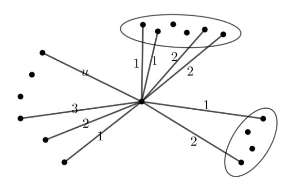
Figure 2. Illustration of a strong rainbow coloring on Amal\((K_{m_1}, \ldots, K_{m_t})\).

3.2. Generalized Wheel Graphs

This is an example in which the \(\omega\) lower bound in Theorem 2.1 is sharper than \(\beta_0\). The join of a cycle with any graph, i.e. \(C_n + H\), is called the generalized wheel graphs. This class of graph has been studied under various labelling schemes [3]. Now we consider the rc and src.

Theorem 3.2. Let \(n \geq 3\) and H be any graph. Then

(1) \(rc(C_n + H) = \min\{3, src(C_n + H)\}.\)

(2) If \[|V(H)| \leq \lceil \frac{n}{3} \rceil\], then \(src(C_n + H) = \lceil \left( \frac{n}{3} \right)^{\frac{1}{|V(H)|}} \rceil\).

Proof. (1) By Theorem 2.6 it is enough to prove \(rc(G) \leq 3\). A rainbow 3-coloring on \(G = C_n + H\) can be produced as follows. Put the color 3 on all edges in \(C_n\). Let the cycle be \(v_1 - v_2 - \cdots - v_n - v_1\) in this order. If i is odd, assign color 1 to all \(v_i - H\) edges. If i is even, assign color 2 to all \(v_i - H\) edges. In this way, any two vertices in H can be connected by a rainbow path with color sequence 1, 3, 2, and any two non-adjacent vertices in \(C_n\) can be connected by a rainbow path with color sequence 1, 2 or 3, 1, 2. So this coloring is rainbow, and \(rc(G) \leq 3\).

(2) Let \(Q = V(C_n)\), b = |V(H)|, and \(k = \lceil \frac{n}{3} \rceil\). Then \(Q^* = C_n^2\) by Lemma 3.1. If n = 3 then |V(H)| = 1 and \(G = K_4\). Now let \(n \ge 4\), so that G is not a complete graph and \(src(G) \ge 2\). The following claim simplifies computation.

Claim: \[\left\lceil \sqrt[b]{\frac{n}{3}} \right\rceil = \left\lceil \sqrt[b]{k} \right\rceil\].

Since \(\frac{n}{3} \leq k\), we have \(\left\lceil \sqrt[b]{\frac{n}{3}} \right\rceil \leq \left\lceil \sqrt[b]{k} \right\rceil\). From \(\left\lceil \sqrt[b]{\frac{n}{3}} \right\rceil \geq \sqrt[b]{\frac{n}{3}}\) we have \(\left\lceil \sqrt[b]{\frac{n}{3}} \right\rceil^b \geq \frac{n}{3}\) and so \(\left\lceil \sqrt[b]{\frac{n}{3}} \right\rceil^b \geq k\). This implies \(\left\lceil \sqrt[b]{\frac{n}{3}} \right\rceil \geq \sqrt[b]{k}\), so \(\left\lceil \sqrt[b]{\frac{n}{3}} \right\rceil \geq \left\lceil \sqrt[b]{k} \right\rceil\). The Claim is proved.

If \(4 \le n \le 6\), then k=2 and \(|V(H)| \in \{1,2\}\), so \(\lceil \sqrt[b]{k} \rceil = 2\) and in this case src(G) = 2. Now let \(n \ge 7\). It is not hard to see that \(\beta_0(C_n^2) = \lfloor \frac{n}{3} \rfloor\) and \(\omega(C_n^2) = 3\). So by the \(\omega\) lower bound in Theorem 2.1 we have \(src(G) \ge \lceil \sqrt[b]{\frac{n}{3}} \rceil = \lceil \sqrt[b]{k} \rceil\). For the upper bound, we quote Theorem 2.3 in [8] stating that

\[src(A+B) \le \max\left\{\Delta(A), \left\lceil i(A)^{\frac{1}{|V(B)|}} \right\rceil, \left\lceil |V(B)|^{\frac{1}{i(A)}} \right\rceil\right\}\] (3.3)

where i(A) is the independent domination number of A, which is the smallest cardinality of a set of independent (pairwise non-adjacent) vertices that are also dominating (i.e. any other vertex is adjacent to at least one of them). We apply this with \(A = C_n\) and B = H. The following figure shows that \(i(C_n) \le k\).

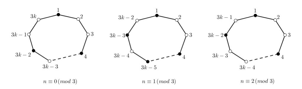
Figure 3. The marked vertices form an independent dominating set of cardinality k.

Remark 3.1. Regardless of the structure of H, we have \(rc(C_n + H) = 3\) when n is sufficiently large, as soon as \(\frac{n}{3} > 2^{|V(H)|}\).

3.3. Sequential Join

This example shows that Theorem 2.2 can be strictly stronger than Theorem 2.1 alone. We will also see some constructive use of color codes. The sequential join of vertex-disjoint graphs \(G_1, G_2, \ldots, G_t\) is defined as the union

\[(G_1 + G_2) \cup (G_2 + G_3) \cup \cdots \cup (G_{t-1} + G_t)\]

denoted by \(G_1 + G_2 + \cdots + G_t\) (see e.g. [3]). We consider on a sequential join of the form \(mK_1 + bK_1 + mK_1\). When b = 1 this graph is a tree so its rc and src are already known. So, we assume \(b \ge 2\).

Theorem 3.3. Let \(G_{m,b} = mK_1 + bK_1 + bK_1 + mK_1\), where \(m \ge 1\), \(b \ge 2\). Let \(n = \lfloor \sqrt[b]{m} \rfloor\). Then

• (1) \(rc(G_{m,b}) = \min\{4, src(G_{m,b})\}.\)
• (2) \(n+1 \le src(G_{m,b}) \le n+3\).

At least two of the values, namely n + 1 and n + 2, can be attained by the src. In fact,

• (i) If \(m \le n^b n + \lfloor \frac{n}{2} \rfloor (2^b 1)\), then \(src(G_{m,b}) = n + 1\).
• (ii) If \(m \ge \min\{(b-1)^b, (n+1)^b (n+1)\}\), then \(src(G_{m,b}) \le n+2\).
• (iii) If \(m \ge (n+1)^b \frac{n}{2}\), then \(src(G_{m,b}) = n+2\).

Proof. Note that \(n^b \leq m < (n+1)^b\). Let \(Q_1 = \{v_1, \ldots, v_m\}\) and \(Q_2 = \{w_1, \ldots, w_m\}\) be the vertex set of the left and right \(mK_1\), with \(CN(Q_1) = \{t_1, \ldots, t_b\}\) and \(CN(Q_2) = \{u_1, \ldots, u_b\}\).

(1) Since \(G_{m,b}\) is bipartite, by Theorem 2.7 it is enough to show \(rc(G_{m,b}) \leq 4\). We construct a rainbow 4-coloring \(\gamma\) on \(G_{m,b}\) as follows. Define \(\gamma\) in such a way so that \(code(v_i) = (1, 2, 2, ..., 2)\)

with respect to \(\{t_1,\ldots,t_b\}\), and \(code(w_i)=(1,4,4,\ldots,4)\) with respect to \(\{u_1,\ldots,u_b\}\), for all \(i \in \{1, \dots, m\}\). The middle part of \(G_{m,b}\) i.e. the subgraph induced by \(CN(Q_1) \cup CN(Q_2)\), is a complete bipartite graph \(bK_1 + bK_1 = K_{b,b}\) whose src is according to [1] equal to \(\lceil \sqrt[b]{b} \rceil = 2\)(because \(1 < b < 2^b\) for b > 2). Put a rainbow 2-coloring on the middle part by using the colors 1 and 3. We modify the coloring in the middle part such that \(\gamma(t_1u_1)=1, \gamma(t_2u_1)=2, \gamma(t_2u_2)=3,\)and \(\gamma(t_1u_2)=4\), without destroying rainbow connectivity. Now we prove that \(\gamma\) is rainbow. Let \(x, y \in V(G_{m,b})\) be non-adjacent.

Case 1: \(x, y \in Q_1\) (or by symmetry \(x, y \in Q_2\)). The path \(x^{\frac{1}{4}}t_1^{\frac{4}{4}}u_2^{\frac{3}{4}}t_2^{\frac{2}{4}}y\) is rainbow.

Case 2: \(x \in Q_1\) and \(y \in CN(Q_2)\) (or by symmetry \(x \in CN(Q_1)\) and \(y \in Q_2\)). The path \(x^2 + t_2 + u_1 + u_1 = u_1\) is rainbow, and so is \(x^2 + u_2 + u_i\) for \(i \in \{2, ..., b\}\).

Case 3: \(x, y \in CN(Q_1)\) (or by symmetry \(x, y \in CN(Q_2)\)). By construction, there is a rainbow path from x to y.

Case 4: \(x\in Q_1\) and \(y\in Q_2\). The path \(x-t_2-u_2-y\) is rainbow. This completes the proof of (1).

To prove (2) and the remaining statements, we need the following claim. Claim: Let \(c \in \mathbb{N}\) satisfy \(m \leq c^b - c + \left| \frac{c}{2} \right| (2^b - 1)\). Then \(src(G_{m,b}) \leq c + d\), where

\[d = \begin{cases} 1, & \text{if } m \ge c^b - c \text{ or } c \ge b, \\ 2, & \text{otherwise.} \end{cases}\] (3.4)

We prove this by constructing a strong rainbow (c+d)-coloring \(\gamma\) on \(G_{m,b}\). Let \(m' \geq m\) be such that \(c^b - c + \left| \frac{c}{2} \right| \le m' \le c^b - c + \left| \frac{c}{2} \right| (2^b - 1)\). Construct \(H = G_{m',b}\) from \(G_{m,b}\) by adding new vertices, extending \(Q_i\) into \(Q_i'\) for all \(i \in \{1, 2\}\). First, we define \(\gamma\) as a coloring on H. Later, we will erase the new vertices and restrict \(\gamma\) to \(G_{m,b}\).

We begin by coloring the middle part, i.e. \(bK_1 + bK_1\) whose src is 2. If d = 2, put a strong rainbow 2-coloring on this part with the colors c+1 and c+2. If d=1, then we put \(\gamma(t_iu_i)=c+1\)instead for all \(i, j \in \{1, 2\}\).

Now we color the left wing. Including \(v_1\), choose any \(c^b - c\) vertices in \(Q'_1\) to form a set \(Q_{11}\). The edges adjacent to \(Q_{11}\) are colored in such a way so that, with respect to \(\{t_1,\ldots,t_b\}\), the set \(code(Q_{11})\) consists of all non-diagonal b-tuples with entries from \(\{1,\ldots,c\}\). If \(c\geq b\), we also put \(code(v_1) = (1, 2, 3, \dots, b)\). Analogously, we form \(Q_{21} \subseteq Q'_2\) and put the coloring in the same way.

Next, for each \(i \in \{1, 2\}\), choose any \(\left|\frac{c}{2}\right|\) vertices from \(Q'_i \setminus Q_{i1}\) and let them form a set \(Q_{i2}\). Put the coloring on edges adjacent to \(Q_{i2}\) so that \(code(Q_{12})\) and \(code(Q_{22})\) are disjoint and their union consists of all diagonal tuples with entries taken from \(\{1,\ldots,2\mid\frac{c}{2}\mid\}\subseteq\{1,\ldots,c\}\).

Finally, for each \(i \in \{1, 2\}\), let \(Q_{i3} = Q_i \setminus (Q_{i1} \cup Q_{i2})\). If \(Q_{i3} = \emptyset\) we are done. Otherwise, put the coloring on edges incident to \(Q_{i3}\) in a way so that \(code(Q_{i3})\) consists of permutations of \((a, a, \ldots, a, c+1, c+1, \ldots, c+1)\), where \(a \in \{1, \ldots, c\}\) with \((a, a, \ldots, a) \in code(Q_{i2})\) is repeated

j times, for some j ∈ {1, . . . , b}. The number of such a tuple (a1, a2, . . . , ab) is precisely

\[\left\lfloor \frac{c}{2} \right\rfloor \sum_{j=1}^{b-1} {b \choose j} = \left\lfloor \frac{c}{2} \right\rfloor (2^b - 2). \tag{3.5}\]

The condition m⁰ ≤ c ^b − c + c 2 (2^b − 1) implies that

\[|Q_{i3}| = m' - (|Q_{i1}| + |Q_{i2}|) = m' - c^b + c - \left\lfloor \frac{c}{2} \right\rfloor \le \left\lfloor \frac{c}{2} \right\rfloor (2^b - 2).\] (3.6)

Therefore, all vertices of Qi³ can be allocated such tuples.

After erasing all the new vertices, we end the definition of γ. Now we prove that γ is strong rainbow. Let x, y ∈ V (Gm,b) be non-adjacent.

Case 1: x, y ∈ Q¹ or x, y ∈ Q²

For each i ∈ {1, 2}, all vertices in Qⁱ have distinct codes. We are done by Lemma 1.1.

Case 2: x ∈ Q¹ and y ∈ CN(Q2) (or by symmetry x ∈ CN(Q1) and y ∈ Q2).

There is i ∈ {1, . . . , b} such that γ(xti) ≤ c. Then x−ti−y is a rainbow geodesic.

Case 3: x, y ∈ CN(Q1) (or by symmetry x, y ∈ CN(Q2)).

Say x = tⁱ and y = t^j with 1 ≤ i < j ≤ b.

Subcase 3.1: m ≥ c ^b − c.

In this subcase the set code(Q11) contains all off-diagonal tuples with entries from {1, . . . , c}, so there is v ∈ Q¹¹ such that the i'th component of code(v) is different than the j'th component. Then x−v−y is a rainbow geodesic.

Subcase 3.2: c ≥ b.

In this subcase code(v1) = (1, 2, . . . , b), so x i −v¹ j −y is a rainbow geodesic.

Subcase 3.3: d = 2.

In this subcase there is a rainbow geodesic between x and y in the middle part (bK¹ + bK1).

In the remaining cases we consider x ∈ Q¹ and y ∈ Q2.

Case 4: x ∈ Q¹¹ and y ∈ Q21.

If code(x) with respect to {t1, . . . , tb} is equal to code(y) with respect to {u1, . . . , ub}, choose i, j ∈ {1, . . . , b} with i 6= j and γ(xti) 6= γ(xt^j ) = γ(yu^j ). Then the geodesic x−ti−uj−y is rainbow. Now suppose that code(x) 6= code(y), say they differ at the i'th component. Then the geodesic x−ti−ui−y is rainbow.

Case 5: x ∈ Q¹¹ and y ∈ Q²² ∪ Q²³ (or by symmetry, x ∈ Q¹² ∪ Q¹³ and y ∈ Q21). There is j ∈ {1, . . . , b} with γ(yu^j ) ≤ c. Since code(x) is non-diagonal, there is i ∈ {1, . . . , b} with γ(xti) 6= γ(yu^j ). Then the geodesic x−ti−uj−y is rainbow.

Case 6: x ∈ Q¹² and y ∈ Q22.

Since code(Q12) ∩ code(Q22) = ∅, code(x) and code(y) are distinct diagonal tuples with entries from {1, . . . , c}. So the geodesic x−t1−u1−y is rainbow.

Case 7: x ∈ Q¹² and y ∈ Q²³ (or by symmetry, x ∈ Q¹³ and y ∈ Q22). Let code(x) = (a, a, . . . , a) and code(y) = (w1, . . . , wb). Let i ∈ {1, . . . , b} be such that

Case 8: \(x \in Q_{13}\) and \(y \in Q_{23}\). Let \(code(x) = (v_1, \ldots, v_b)\) and \(code(y) = (w_1, \ldots, w_b)\). Let \(i, j \in \{1, \ldots, b\}\) be such that \((v_i, v_i, \ldots, v_i) \in code(Q_{12})\) and \((w_j, w_j, \ldots, w_j) \in code(Q_{22})\). Then \(v_i \neq w_j\) since \(code(Q_{12}) \cap code(Q_{22}) = \emptyset\), so the geodesic \(x^{v_i}_{-i}t_i - u_j^{w_j}_{-j}y\) is rainbow. This completes the proof of the Claim.

• (2) From Theorem 2.1 with \(Q=Q_1\cup\{u_1\}\), we have \(src(G_{m,b})\geq\sqrt[b]{m+1}>n\). So we get the lower bound \(src(G_{m,b})\geq n+1\). Let c=n+1. Note that \(\left\lfloor\frac{n+1}{2}\right\rfloor(2^b-1)\geq 3\left\lfloor\frac{n+1}{2}\right\rfloor\geq n+1\). So \(c^b-c+\left\lfloor\frac{c}{2}\right\rfloor(2^b-1)\geq c^b=(n+1)^b>m\), and the Claim gives \(src(G_{m,b})\leq c+2=n+3\).
• (i) If \(m \le n^b n + \left\lfloor \frac{n}{2} \right\rfloor\) \((2^b 1)\), use the Claim with c = n and d = 1 to obtain \(src(G_{m,b}) \le n + 1\). This and the lower bound \(src(G_{m,b}) \ge n + 1\) prove (i).
• (ii) If \(m \ge \min \{(b-1)^b, (n+1)^b (n+1)\}\), then the Claim with c = n+1 and d = 1 gives \(src(G_{m,b}) \le n+2\).
• (iii) Now suppose \(m \ge (n+1)^b \frac{n}{2}\). Then \(m \ge (n+1)^b (n+1)\), so by (ii) we have \(src(G_{m,b}) \le n+2\). Next we use Theorem 2.2 with \(Q_1\) and \(Q_2\) with the initial estimate \(src(G_{m,b}) \ge n+1\) to obtain \(src(G_{m,b}) \ge 1 + \left\lfloor \sqrt[b]{m+\frac{n}{2}} \right\rfloor \ge 1 + \left\lfloor \sqrt[b]{(n+1)^b} \right\rfloor = n+2\).

Remark 3.2. As a result, we have \(rc(G_{m,b}) = 4\) when m is sufficiently large compared to b, as soon as \(m \ge 3^b\).

When b = 2, we have a complete solution for the rc.

Theorem 3.4. \[rc(G_{m,2}) = \begin{cases} 3, & \text{if } 1 \leq m \leq 5, \\ 4, & \text{if } m \geq 6. \end{cases}\]

Proof. We continue to use the same notation as in the proof of previous theorem. If \(1 \le m \le 3\), then by Theorem 3.3(2) we have \(rc(G_{m,2}) \le src(G_{m,2}) \le \lfloor \sqrt{m} \rfloor + 2 = 3\). If \(4 \le m \le 5\), then Theorem 3.3(1) gives \(rc(G_{m,2}) \le src(G_{m,2}) = \lfloor \sqrt{m} \rfloor + 1 = 3\). Now let \(m \ge 6\) and suppose \(rc(G_{m,2}) \le 3\). Then there is a rainbow 3-coloring \(\gamma\) on \(G_{m,2}\).

Claim 1: For any \(i \in \{1, 2\}\), all vertices in \(code(Q_1) \cup \{u_i\}\) have different codes with respect to \(\{t_1, t_2\}\). Also, all vertices in \(code(Q_2) \cup \{t_i\}\) have different codes with respect to \(\{s_1, s_2\}\).

A path between vertices in \(Q_1 \cup \{u_i\}\) not passing through \(t_1\) or \(t_2\) has length at least 4. So, any rainbow path between vertices in \(Q_1 \cup \{u_i\}\) must be of the form \(x-t_i-y\). This proves Claim 1.

Claim 2: There is at least one diagonal tuple in \(code(Q_1)\), and at least one in \(code(Q_2)\).

Assume otherwise. Suppose \(code(Q_1)\) has no diagonal tuple. Since there are only six non-diagonal tuples, we have m=6 and \(code(Q_1)=\{(1,2),(2,1),(1,3),(3,1),(2,3),(3,2)\}\). By Claim 1, the codes of \(u_1\) and \(u_2\) with respect to \(\{t_1,t_2\}\) are both diagonal. If \(code(u_1)\neq code(u_2)\), say \(code(u_1)=(1,1)\) and \(code(u_2)=(2,2)\), then there are no rainbow path from the vertex in \(Q_1\) with code (1,2) to any vertex in \(Q_2\). Now suppose \(code(u_1)=code(u_2)\), say (1,1). There is some \(x\in Q_2\) with \(code(x)\in\{(1,2),(1,3),(2,1),(3,1)\}\), because otherwise \(code(Q_2)\subseteq\)

{(1, 1),(2, 2),(3, 3),(2, 3),(3, 2)}. Let y ∈ Q² with code(y) = code(x). Then there are no rainbow paths between x and y. The proof of Claim 2 is complete.

Claim 3: There is at most one diagonal tuple in code(Q1), and at most one in code(Q2).

Assume otherwise. WLOG, let a, b ∈ Q¹ with code(a) = (1, 1) and code(b) = (2, 2). If there is some c ∈ Q² with code(c) ∈ {(1, 1),(2, 2)}, then there are no rainbow paths between c and a, or between c and b. So code(Q2) ⊆ {(3, 3),(1, 2),(2, 1),(1, 3),(3, 1),(2, 3),(3, 2)}.

Case 1: (3, 3) ∈ code(Q2).

Suppose c ∈ Q² with code(c) = (3, 3). There is a rainbow path from a to c, so γ(tiu^j ) = 2 for some i, j ∈ {1, 2}. By symmetry, we may assume γ(t1u1) = 2. Consider code(u1) = (2, γ(u1t2)) with respect to {t1, t2}. By Claim 1, code(u1) 6∈ code(Q1). So code(u1) 6= (2, 2).

Subcase 1.1: code(u1) = (2, 1).

Since |code(Q2)\{(3, 3)}| ≥ 5, at least one of (1,2) or (2,1) is in code(Q2). If x ∈ Q² with code(x) = (1, 2), then there are no rainbow path from x to b. If x ∈ Q² with code(x) = (2, 1), then there are no rainbow path from x to a.

Subcase 1.2: code(u1) = (2, 3).

There is a rainbow path from c to b, so either γ(u2t1) = 1 or γ(u2t2) = 1.

Subsubcase 1.2.1: γ(u2t1) = 1.

Since |code(Q2)\{(3, 3)}| ≥ 5, at least one of (1,2) or (2,1) is in code(Q2). If x ∈ Q² with code(x) = (1, 2), then because there is a rainbow path from x to a, we must have γ(t2u2) = 3. If x ∈ Q² with code(x) = (2, 1), then because there is a rainbow path from x to b, we must have γ(t2u2) = 3. In either case, code(t2) = (3, 3) with respect to {u1, u2}, contradicting Claim 1.

Subsubcase 1.2.2: γ(u2t2) = 1.

Now code(t2) = (3, 1) with respect to {u1, u2}, so by Claim 1 and |code(Q2)\{(3, 3)}| ≥ 5 we must have code(Q2) = {(3, 3),(1, 2),(2, 1),(1, 3),(2, 3),(3, 2)}. Let x ∈ Q² with code(x) = (1, 3). There must be a rainbow path from x to a, so γ(u2t1) = 2. Then there are no rainbow paths from a to the vertex in Q² whose code is (1, 2).

Case 2: (3, 3) 6∈ code(Q2).

Since m ≥ 6, in this case code(Q2) = {(1, 2),(2, 1),(1, 3),(3, 1),(2, 3),(3, 2)}. Let x ∈ Q² with code(x) = (1, 3). There must be a rainbow path from x to a, so either γ(u2t1) = 2 or γ(u2t2) = 2. By symmetry, we may assume γ(u2t2) = 2. By Claim 1, code(t2) with respect to {u1, u2} cannot be an non-diagonal tuple, so code(t2) = (2, 2).

Now let y ∈ Q² with code(y) = (2, 1). There must be a rainbow path from y to b, so γ(u2t1) = 3. Because code(t1) with respect to {u1, u2} cannot be an non-diagonal tuple, we must have code(t1) = (3, 3). Then there are no rainbow paths from b to the vertex in Q² whose code is (3,2). This completes the proof of Claim 3.

Now, by Claim 2 and Claim 3, there is exactly one diagonal tuple in code(Q1), and similarly in code(Q2). By Claim 1, this forces m ≤ 7, each of code(Q1) and code(Q2) can only miss at most one non-diagonal tuple, and at most one non-diagonal tuple can occur as code(u1) or code(u2).

WLOG, let us assume (1, 1) ∈ code(Q1), say x ∈ Q¹ with code(x) = (1, 1). If none of code(u1), code(u2) is equal to (2,2) or (3,3), then code(u1) = code(u2) = (a, b) with a 6= b.

But then code(t1) = (a, a) and code(t2) = (b, b). Therefore, exchanging the role of Q¹ and Q² if necessary, we may assume without loss of generality that (1, 1) ∈ code(Q1) and code(u1) = (2, 2).

If (2, 1) ∈ code(Q2), then there are no rainbow paths from x to the vertex in Q² whose code is (2,1). So (2, 1) 6∈ code(Q2). Hence, all non-diagonal tuples except (2,1) are in code(Q2). In particular, there is some y ∈ Q² with code(y) = (1, 2).

Because there is a rainbow path from x to y, we must have γ(t1u2) = 3 or γ(t2u2) = 3. So either code(t1) = (2, 3) or code(t2) = (2, 3), contradicting Claim 1 since (2, 3) ∈ code(Q2).

References

• [1] G. Chartrand, G.L. Johns, K.A. McKeon and P. Zhang. Rainbow connection in graphs, Math. Bohem. 133 (2008), 85–98.
• [2] D. Fitriani and A.N.M. Salman. Rainbow connection number of amalgamation of some graphs. AKCE Int. J. Graphs Comb. 13 (2016), 90–99.
• [3] J.A. Gallian. A dynamic survey of graph labelling. Electron. J. Combin. 17 (2014).
• [4] T.W. Haynes, S.T. Hedetniemi and P.J. Slater. Fundamentals of domination in graphs, Marcell Dekker Inc, 1998.
• [5] X. Li and Y. Sun. On strong rainbow connection number. arXiv:1010.6139 [math.CO] 2010.
• [6] X. Li and Y. Sun. Rainbow connections of graphs, Springer, 2012.
• [7] I. Schiermeyer, Bounds for the rainbow connection number of graphs, Discuss. Math. Graph Theory 31 (2011), 387–395.
• [8] F. Septyanto and K.A. Sugeng. Rainbow connections of graph joins, Australas. J. Combin.: Special Issue in Memory of Mirka Miller, 69 (3) (2017), 375–381.