Interlace polynomials of friendship graphs

Christina Eubanks-Turner^a , Aihua Li^b

^aDepartment of Mathematics, Loyola Marymount University, 90045

ceturner@lmu.edu, lia@mail.montclair.edu

In this paper, we study the interlace polynomials of friendship graphs, that is, graphs that satisfy the Friendship Theorem given by Erdos, R ¨ enyi and Sos. Explicit formulas, special values, and ´ behaviour of coefficients of these polynomials are provided. We also give the interlace polynomials of other similar graphs, such as, the butterfly graph.

Keywords: graph polynomial, interlace polynomial, friendship graph, butterfly graph

Mathematics Subject Classification : 05C31, 05C50

DOI: 10.5614/ejgta.2018.6.2.7

1. Introduction

Sequencing by hybridization is a method of reconstructing a long DNA string from its nucleotide sequence. Since gaining a unique reconstruction from the substrings is not always possible, a major question that arises in this study is "For a random string, how many reconstructions are possible?" In [2], Arratia, Bollobas, Coppersmith, and Sorkin answer an important question ´ related to DNA sequencing by converting this to a question about Euler circuits in a 2-in, 2-out graph that have been "toggled" (interlaced). The previously mentioned authors introduced the interlace polynomial of a graph, a polynomial that represents the information gained from doing the toggling process on the graph, see [2]. Interlace polynomials are similar to other graph polynomials, such as, Tutte and Martin polynomials, see [5]. Some researchers have studied different types of graph polynomials, such as genus polynomials, [7].

Received: 09 September 2017, Revised: 30 May 2018, Accepted: 16 June 2018.

^bDepartment of Mathematical Sciences, Montclair State University, 07043

An interlace polynomial gives important information about the graph, for example, the number of k-component circuit partitions, for any k ∈ N. In [3], interlace polynomials for some simple graphs like paths, cycles, and complete graphs are given although not all of the formulas are easy to use. Li, Wu and Nomani give recursive formulas for interlace polynomials of ladder and n-Claw graphs, see [8, 9]. More recently, work has been done in utilizing bivariate and multi-variate interlace polynomials, see [1, 3, 10]. Here, we focus our attention on establishing the interlace polynomials of graphs with certain structures. In particular, we study the interlace polynomials of friendship graphs.

A friendship graph is a graph that satisfies the Friendship Theorem given by Erdos, R ¨ enyi and ´ Sos in [6]. These graphs are also sometimes called fan or windmill graphs. The friendship graph Fⁿ with n 3-cycles is a graph that models other scientific phenomena in computer networks and political science. Here we give both the recursive and explicit formulas for the interlace polynomials of friendship graphs. As Li and Wu did for ladder graphs in [8], we consider natural questions regarding interlace polynomials of friendship graphs:

• 1. What does each coefficient of the interlace polynomial of a friendship graph tell us about the graph?
• 2. Will evaluating the interlace polynomial of a friendship graph at certain values describe some related graph property?

We also examine the above questions for another type of graph related to the friendship graph. The butterfly graph is a graph with 6 vertices and 5 edges that consists of two 3-cycles adjoined at a common vertex. In this paper we develop both recursive and explicit formulas for graphs consisting of paths of butterfly graphs.

For a simple graph G, to construct the interlace polynomial we first need the following definition. Note that for any vertex a ∈ V (G), define N(a) = {b ∈ V (G)|(a, b) ∈ E(G)}.

Definition 1.1. (Pivot) Let G = (V (G), E(G)) be any undirected graph without a loop and a, b ∈ V (G) with ab ∈ E(G). We first partition the neighbors of a or b into three classes:

• 1. N(a) \ ({b} ∪ N(b));
• 2. N(b) \ ({a} ∪ N(a));
• 3. N(a) ∩ N(b).

The pivot graph Gab of G, with respect to ab is the resulting graph of the toggling process: ∀u, v ∈ V (G), if u, v are from different classes shown above, then uv ∈ E(G) ⇐⇒ uv /∈ E(Gab).

Note that Gab = Gba. The pivot operation is only defined for an edge of G. The definition for the interlace polynomial of a simple graph G is given below. Here, ∀u ∈ V (G), G − u is the graph resulting from removing u and all the edges of G incident to u from G.

Definition 1.2. For any undirected graph G with n vertices, the interlace polynomial q(G, x) of G is defined by

\[q(G,x) = \begin{cases} x^n, & \text{if } E(G) = \emptyset \\ q(G-a,x) + q(G^{ab}-b,x), & \text{if } ab \in E(G). \end{cases}\]

By a theorem in [2], this map is a well-defined polynomial on all simple graphs. We also give some known results about interlace polynomials and results relating the interlace polynomials to structural components of graphs.

Lemma 1.3. [3] Given the interlace polynomial q(G, x) of any undirected graph G, the following results hold:

• 1. The interlace polynomial of any simple graph has zero constant term.
• 2. For any two disjoint graphs G1, G2, we have q(G¹ ∪ G2, x) = q(G1, x) · q(G2, x).
• 3. The degree of the lowest-degree term of q(G, x) is k(G), the number of components of G.
• 4. deg(q(G, x)) ≥ α(G), where α(G) is the independence number, i.e., the size of a maximum independent set.
• 5. Let µ(G) denote the size of a maximum matching (maximum set of independent edges) in a graph G. If G is a forest with n vertices, then deg(q(G, x)) = n − µ(G).

Lemma 1.4. [3] The interlace polynomials for the following graphs are as follows:

• 1. (complete graph Kn) q(Kn, x) = 2ⁿ−¹x;
• 2. (complete bipartite graph Kmn) q(Kmn, x) = (1 + x + ... + x m−1 )(1 + x + ... + x n−1 ) + x ^m + x ⁿ − 1;
• 3. (path Pⁿ with n edges) q(P1, x) = 2x, q(P2, x) = x ² + 2x, and for n ≥ 3, q(Pn, x) = q(Pn−1, x) + xq(Pn−2, x);
• 4. (small cycles Cn) q(C3, x) = 4x and q(C4, x) = 2x + 3x 2 .

In [3], Arrati, Bollobas and Sorkin give a list of open problems and conjectures related to ´ interlace polynomials. Similar conjectures have been raised about other graph polynomials, such as the chromatic polynomial. If solved, some of these conjectures can give information about circuit counting in graphs. We show that the following conjecture given in [3], a conjecture about unimodal coefficients holds for friendship graphs, see Proposition 2.6.

Conjecture 1.5. [3] For any graph G, the sequence of coefficients of q(G, x) is unimodal: nondecreasing up to some point, then non-increasing. The associated polynomial xq(G, 1+x) likewise has unimodal coefficients.

In 1966, Erdos, R ¨ enyi and Sos proved the Friendship theorem. Since then others have given ´ alternate proofs of the theorem. Below we state the theorem.

Theorem 1.6. [6] Suppose G is a finite graph where any two vertices share exactly one neighbor. Then there is a vertex adjacent to all other vertices.

Note, in [6] it is shown that every friendship graph is a windmill graph.

Definition 1.7. Let n ∈ N. The friendship graph Fⁿ is the simple graph with 2n + 1 vertices and 3n edges that satisfies Theorem 1.6.

The graph Fⁿ is obtained by joining n copies of the cycle C³ at a common vertex. Below is an example of the friendship graph with n = 4.

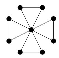
Figure 1. The graph F4.

2. Interlace Polynomial of Friendship Graphs

Next, we develop interlace polynomials of friendship graphs Fn, where n ∈ N. We treat F⁰ = E1, the one vertex graph.

Lemma 2.1. For \[n \ge 1\], \(q(\mathcal{F}_n, x) = 2q(\mathcal{F}_{n-1}, x) + 2^n x^n\).

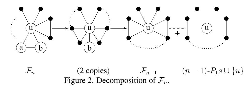
Proof. Obviously q(F0, x) = x and q(F1, x) = 4x. For n ≥ 2, we toggle Fⁿ at an edge of a triangle incident only to vertices of degree 2. It decomposes into 2 copies of q(Fn−1, x) attached by b as a leaf adjacent to u. Next we toggle the edge ub on the resulting graph. This produces n disconnected copies of P¹ and the graph E¹ the vertex u, see Figure 2. Thus,

\[q(\mathcal{F}_n, x) = 2(q(F_{n-1}, x) + x(2x)^{n-1}) = 2q(F_{n-1}, x) + 2^n x^n.\]

We give a picture to help better illustrate the proof of Lemma 2.1. We symbolize the center vertex as u.

Theorem 2.2. For ^{n ≥ 0}, the interlace polynomial of ^Fn is given by ^q(Fn, x) = ^Xn k=1 2 nx ^k + 2ⁿx. In particular,

\[q(\mathcal{F}_n, x) = 2^n \left( \frac{x^{n+1} - 1}{x - 1} + x - 1 \right)\]

when x 6= 1 and q(Fn, 1) = (n + 1)2ⁿ .

Proof. We proceed by induction. Note, ^q(F0, x) = ^x = 2⁰x. Now assume ^q(Fn, x) = ^Xn k=1 2 nx ^k + 2 ⁿx for all n ≥ 0, and consider q(Fn+1, x). By Lemma 2.1 and the inductive hypothesis we have, q(Fn+1, x) = 2q(Fn, x) + 2ⁿ+1x ⁿ+1 = 2[2ⁿ (x ⁿ + x ⁿ−¹ + . . . + x ² + 2x)] + 2ⁿ+1x ⁿ+1 = 2 ⁿ+1(x ⁿ+1 + x ⁿ + . . . + x ² + 2x). Thus the result holds for all n ≥ 0. Using the geometric sum n

formula, ^q(Fn, x) = ² (x ⁿ+1 − 1) x − 1 + 2ⁿ (x − 1), when x 6= 1.

In [3] Arritia, Bollobas and Sorkin evaluate some interlace polynomials at small ´ x-values. They show that for any graph G, q(G, 2) = 2^|V (G)^| . They also gave a conjecture about the explicit formula of the interlace polynomial at x = −1. In the folllowing Theorem Balister, Bollobas, ´ Cutler and Peabody gives an explicit formula for the interlace at x = −1, therefore proving the conjecture in [4].

Theorem 2.3. [4] Let A be the adjacency matrix of G, n = |V (G)| and let r = rank(A + I) over Z² and I be the n × n identity matrix. Then

\[q(G,-1) = (-1)^n (-2)^{n-r}.\]

By Theorem 2.2 we claim the following about the interlace of Fn, for n ≥ 0.

Corollary 2.4. Let n ≥ 0. Then q(Fn, 2) = 2²n+1 and

\[q(\mathcal{F}_n, -1) = \begin{cases} -2^n, & \text{if } n \text{ is even} \\ -2^{n+1}, & \text{if } n \text{ is odd} \end{cases}\]

Proof. Using Theorem 2.2, we have ^q(Fn, x) = ² n (x ⁿ+1 − 1) x − 1 + 2ⁿ (x − 1), when x 6= 1, and so q(Fn, 2) = 2ⁿ (2ⁿ+1 − 1) + 2ⁿ = 2²n+1 = 2^|V (Fn)^| , confirming the exiting result from [3]. Also, by Theorem 2.2,

\[q(\mathcal{F}_n, -1) = \frac{2^n((-1)^{n+1} - 1)}{-2} - 2^{n+1} = 2^{n-1}[(-1)^n - 3]\]

and so the claim holds.

Similar to [3], we give some brief properties that relate q(Fn, x) to the independence and matching number of the graph Fn. Note, |V (Fn)| = 2n + 1 and |E(Fn)| = 3n.

Lemma 2.5. For n > 0, α(Fn) = µ(Fn) = n, where α is the independence number and µ is the size of the maximum matching.

Proof. By (4) of Lemma 1.3 we have that deg(q(Fn, x)) ≥ α(Fn) and so α(Fn) ≤ n. This implies α(Fn) = n since one can exhibit an independent set of size n by taking exactly one vertex of degree 2 on each triangle of Fn. Also, µ(Fn) = n by taking the matching that consists of all edges not adjacent to the vertex of maximum degree in Fn.

Now we verify that q(Fn, x) satisfies Conjecture 1.5 given in [3].

Proposition 2.6. For \(n \geq 0\), the coefficients of both \(q(\mathcal{F}_n, x)\) and \(xq(\mathcal{F}_n, 1+x)\) are unimodal.

Proof. By Theorem 2.2 \(q(\mathcal{F}_n, x) = 2^n x + \sum_{k=1}^n 2^n x^k\) and so it is clear that the sequence of coefficients of \(q(\mathcal{F}_n, x)\) is unimodal. Considering \(xq(\mathcal{F}_n, 1+x)\), we have,

\[xq(\mathcal{F}_n, 1+x) = 2^n x \left( (1+x) + \sum_{k=1}^n (1+x)^k \right)\] \[= 2^n (x^2+x) + 2^n \sum_{k=1}^n \left( \sum_{j=0}^n \binom{k}{j} x^{j+1} \right)\] \[= 2^n (x^2+x) + 2^n (nx) + 2^n \sum_{j=1}^n \left( \sum_{k=j}^n \binom{k}{j} \right) x^{j+1}\] \[= 2^n (n+1)x + 2^n \left( 1 + \binom{n+1}{2} \right) x^2 + 2^n \sum_{j=2}^n \binom{n+1}{j+1} x^{j+1}.\]

Therefore, the sequence of coefficients of \(xq(F_n, 1+x)\) in the order of \(x^{n+1}\) down to x is

\[2^{n} \binom{n+1}{n+1}, 2^{n} \binom{n+1}{n}, \cdots, 2^{n} \binom{n+1}{3}, 2^{n} \left(1 + \binom{n+1}{2}\right), 2^{n} (n+1),\]

and so \(xq(\mathcal{F}_n, 1+x)\) is unimodal for \(n \geq 0\).

Now we consider applications of friendship graphs in solving a linear algebra problem. We determine the ranks of the adjacency matrices associated with \(\mathcal{F}_n\) over \(\mathbb{Z}_2\). For \(n \geq 1\), let \(A_n\) denote the adjacency matrix of \(\mathcal{F}_n\). Then

\[A_n = \begin{pmatrix} 0 & 1 & 1 & \dots & 1 \\ 1 & I' & & & & \\ 1 & & I' & & & & \\ & & & & \ddots & & \\ 1 & & \mathbf{0} & & & I' \end{pmatrix}_{(2n+1) \times (2n+1)}\]

where \(I' = \begin{pmatrix} 0 & 1 \\ 1 & 0 \end{pmatrix}\).

Next we give a result related to Theorem 2.3, which references the matrix \(R_n = A_n + I_{2n+1}\).

Note that

\[R_n = \begin{pmatrix} 1 & 1 & 1 & \dots & 1 \\ 1 & I_0 & & & & \\ 1 & & I_0 & & & & \\ & & & & & & \\ 1 & & 0 & & & & \\ & & & & & & \\ 1 & & 0 & & & & I_0 \end{pmatrix}_{(2n+1)\times(2n+1)}\]

where \(I_0 = I_2 + I' = \begin{pmatrix} 1 & 1 \\ 1 & 1 \end{pmatrix}\).

Proposition 2.7. For \(n \geq 1\). Let \(A_n\) be the adjacency matrix of \(\mathcal{F}_n\) and \(R_n = A_n + I_{2n+1}\). Then

\[rank(R_n) = \begin{cases} n+1, & \text{if } n \text{ is even} \\ n, & \text{if } n \text{ is odd.} \end{cases}\]

Proof. Let \(r = rank(R_n)\) over \(\mathbb{Z}_2\). As \(\mathcal{F}_n\) has 2n+1 vertices, by Theorem 2.3 and Corollary 2.4 we have \(q(\mathcal{F}_n,-1)=(-1)^{2n+1}(-2)^{2n+1-r}=(-1)^r2^{2n+1-r}\). Since \(q(\mathcal{F}_n,-1)<0\), for all \(n\geq 0\), r must be odd and so \(q(\mathcal{F}_n,-1)=-2^{2n+1-r}\). When n is even, \(-2^{2n+1-r}=-2^n\) and so r=n+1. When n is odd, \(-2^{2n+1-r}=-2^{n+1}\) and so r=n.

Theorem 2.8. Let \(A_n\) be the adjacency matrix of \(\mathcal{F}_n\), \(n \geq 1\). Then \(rank(A_n) = 2n\) over \(\mathbb{Z}_2\).

Proof. Since the first column of \(A_n\) is the sum of columns 2 through 2n + 1, replacing the first column with the sum of columns 1 through 2n + 1, we get the first column as the zero column. Then replacing the first row with the sum of rows 1 through 2n + 1, we have the resulting matrix:

\[\text{[rumus tidak dapat ditampilkan dengan baik — lihat PDF asli]}\]

Since each I' has rank 2 over \(\mathbb{Z}_2\), \(rank(A'_n)=2n\) and so \(rank(A_n)=2n\).

3. Interlace Polynomials of Butterfly Path Graphs

Now we turn our attention to graphs similar to friendship graphs. The butterfly graph also known as the bowtie graph or hourglass graph is an undirected, planar graph. The figure below illustrates the butterfly graph. We consider the butterfly graph since it is also \(\mathcal{F}_2\), a friendship

graph. Note that the friendship graph F² is actually the butterfly graph B1. The graph B¹ has one cut vertex, the vertex of degree 4. When n = 2k is even, the graph Fⁿ is the result of gluing k butterfly graphs B¹ at the cut vertices. Furthermore, the graph Bⁿ can be viewed as a "path" of B¹ s. It is also a molecular graph reflecting certain molecular structures. The graph Dⁿ is the resulting graph by removing two end triangles of Bn. It can be used to develop a recursive formula for the interlace polynomial of Bn. In this section we explore the interlace polynomials of a graphs we call Bn, the "path" of n butterfly graphs. Here we treat B⁰ = P1, the path with one edge.

Figure 3. The Butterfly graph (B1).

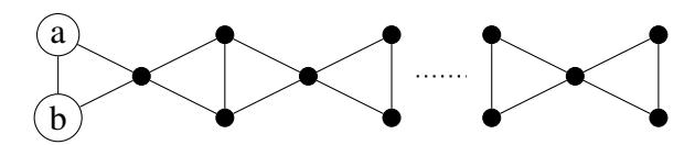
For n ≥ 1, let Bⁿ be the graph made of n B1-subgraphs, as a path of B1s, see Figure 4.

Figure 4. The graph Bⁿ which contains n-B¹ graphs.

We name these graphs Bⁿ because each of them is an extension of the butterfly graph. For n > 1, Bⁿ is no longer a friendship graph. To build iterative formulas for interlace polynomials q(Bn, x), we use graphs Dn, where each Dⁿ is a graph obtained by adding a triangle at one end of Bⁿ (adding two additional edges). We let D⁰ = C3, the cycle with three edges. Therefore, Dⁿ has the form as in Figure 5.

Figure 5. The Graph of Dn, which contains n-B¹ graphs.

Theorem 3.1. For \[n \ge 1\], \(q(B_n, x) = 2xq(B_{n-1}, x) + 2q(D_{n-1}, x)\) and \(q(D_n, x) = q(B_n, x) + 2xq(D_{n-1}, x)\).

Proof. Pick an edge of Bⁿ where each end vertex has degree 2. Call the vertices of this edge a and b. So we have:

Then by toggling along this edge we decompose Bⁿ into two copies of the following graph that now has as its maximum butterfly path Bn−1:

Interlace polynomials of friendship graphs | C. Eubanks-Turner and A. Li

Then toggling the edge incident to b, we obtain \(q(B_n, x) = 2xq(B_{n-1}, x) + 2q(D_{n-1}, x)\). Similarly, it follows that \(q(D_n, x) = q(B_n, x) + 2xq(D_{n-1}, x)\).

We compute small values of \(q(B_n, x)\) and \(q(D_n, x)\).

Lemma 3.2. Noting that \(B_0 = P_1\), \(q(B_0, x) = 2x\) and by Lemma 1.4 \(q(D_0, x) = 4x\). By Theorem 3.1, we obtain the following explicit forms:

1. \(q(B_0, x) = x\), \(q(D_0, x) = 4x\)2. \(q(B_1, x) = 4x^2 + 8x\), \(q(D_1, x) = 12x^2 + 8x\)3. \(q(B_2, x) = 8x^3 + 40x^2 + 16x\), \(q(D_2, x) = 32x^3 + 56x^2 + 16x\)4. \(q(B_3, x) = 16x^4 + 144x^3 + 144x^2 + 32x\), \(q(D_3, x) = 80x^4 + 256x^3 + 176x^2 + 32x\)

Immediately we can claim the degrees of the two polynomials.

Corollary 3.3. For all \(n \ge 0\), \(q(B_n, x)\) and \(q(D_n, x)\) are both of degree n + 1.

Proof. We proceed with proof by induction on n. Obviously, \(\deg(q(B_0,x))=1=\deg(q(D_0,x))\). Assume \(\deg(q(B_{n-1},x))=\deg(q(D_{n-1},x))=n\), when \(n\geq 1\). By Theorem 3.1, \(q(B_n,x)=2xB_{n-1}(x)+2q(D_{n-1},x)\) and so \(\deg(q(B_n,x))\geq \deg(q(B_{n-1},x))+1\) since all involved terms have nonnegative coefficients. By induction hypothesis, degree of \(q(D_{n-1},x)\) is n, less than \(\deg(q(B_{n-1},x))+1=n+1\). Thus \(\deg(q(B_n,x))=\deg(q(B_{n-1},x))+1=n+1\). Similarly, \(\deg(q(D_n,x))=n+1\). Therefore, \(\deg(q(B_n,x))=\deg(q(D_n,x))=n+1\) for all \(n\geq 0\). \(\square\)

Applying Theorem 3.1 we have the following theorem.

Theorem 3.4. For \(n \geq 2\),

\[q(B_n, x) = (4x + 2)q(B_{n-1}, x) - 4x^2q(B_{n-2}, x).\]

Proof. One can easily check that for n=2, \(q(B_2,x)=(4x+2)q(B_1,x)-4x^2q(B_0,x)\). For \(n\geq 2\), by Theorem 3.1, we have \(q(B_n,x)=2xq(B_{n-1},x)+2q(D_{n-1},x)\) and so \(q(D_{n-1},x)=\frac{1}{2}q(B_n,x)-xq(B_{n-1},x)\), which implies \(q(D_n,x)=\frac{1}{2}q(B_{n+1},x)-xq(B_n,x)\). Using the latter and Theorem 3.1, we have

\[\frac{1}{2}q(B_{n+1},x) - xq(B_n,x) = q(B_n,x) + x(q(B_n,x) - 2xq(B_{n-1},x)).\]

This implies \(q(B_{n+1}, x) = (4x + 2)q(B_n, x) - 4x^2q(B_{n-1}, x)\).

Now we consider \(q(B_n, x)\) in terms of its coefficients. This gives us a way to describe the relations between coefficients.

Proposition 3.5. For n ≥ 1, we have q(Bn, x) =

\[2^{n+1}x^{n+1} + \sum_{k=3}^{n} (4b_{n-1,k-1} + 2b_{n-1,k} - 4b_{n-2,k-2})x^{k} + 2^{n+1}(4n-3)x^{2} + 2^{n+2}x.\]

Proof. Note that by Theorem 3.4 we have q(Bn, x) = (4x + 2)q(Bn−1, x) − 4x 2 q(Bn−2, x), when n ≥ 2. To prove the result we show each of the following claims by induction on n, where n ≥ 1: Claim 1: bn,n+1 = 2ⁿ+1; Claim 2: bn,¹ = 2ⁿ+2; Claim 3: bn,² = 2ⁿ+1(4n − 3).

Proof of Claim 1: When n = 1, by Lemma 3.2 we can see that b1,² = 4 = 21+1. Assume the statement holds for all k, 1 ≤ k ≤ n − 1. By Theorem 3.4 and the inductive hypothesis we have bn,n+1 = 4bn−1,n − 4bn−2,n−¹ = 4(2ⁿ ) − 4(2ⁿ−¹ ) = 2ⁿ+1 .

Proof of Claim 2: Again by Lemma 3.2 b1,¹ = 8 = 21+2 and so bn,¹ = 2ⁿ+2, when n = 1. Assume the statement holds for all k, 1 ≤ k ≤ n − 1. Therefore, bn,¹ = 2bn−1,¹ = 2(2ⁿ+1) = 2ⁿ+2 .

Proof of Claim 3: By Lemma 3.2 b1,² = 4 = 21+1(4(1) − 3) and so the statement is true for n = 1. Assume the statement holds for all k, 1 ≤ k ≤ n − 1. By Theorem 3.4, bn,² = 4bn−1,¹ + 2bn−1,² and so

\[b_{n,2} = 4b_{n-1,1} + 2b_{n-1,2} = 2^{n+3} + 2(2^n(4(n-1) - 3)) = 2^{n+1}[4 + 4n - 7] = 2^{n+1}(4n - 3).\]

Therefore, using Theorem 3.4 and the claims above we have:

\[\sum_{k=1}^{n+1} b_{n,k} x^k = (4x+2) \sum_{k=1}^{n} b_{n-1,k} x^k - 4x^2 \sum_{k=1}^{n-1} b_{n-2,k} x^k\] \[= \sum_{k=2}^{n+1} 4b_{n-1,k-1} x^k + \sum_{k=1}^{n} 2b_{n-1,k} x^k - \sum_{k=3}^{n+1} 4b_{n-2,k-2} x^k\] \[= (4b_{n-1,n} - 4b_{n-2,n-1}) x^{n+1}\] \[+ \sum_{k=3}^{n} (4b_{n-1,k-1} + 2b_{n-1,k} - 4b_{n-2,k-2}) x^k\] \[+ (4b_{n-1,1} + 2b_{n-1,2}) x^2 + 2b_{n-1,1} x\] \[= 2^{n+1} x^{n+1} + \sum_{k=3}^{n} (4b_{n-1,k-1} + 2b_{n-1,k} - 4b_{n-2,k-2}) x^k\] \[+ 2^{n+1} (4n-3) x^2 + 2^{n+2} x.\]

In summary, for n ≥ 1, Proposition 3.5 gives the following information about important coefficients of q(Bn, x):

1. bn,n+1 = the leading coefficient of q(Bn, x) = 2ⁿ+1 .

• 2. \(b_{n,1}\) = the coefficient of x in \(q(B_n, x) = 2^{n+2}\).
• 3. \(b_{n,2}\) = the coefficient of \(x^2\) in \(q(B_n, x) = 2^{n+1}(4n-3)\).
• 4. For n > 2 and 2 < k < n+1, \(b_{n,k} = 4b_{n-1,k-1} + 2b_{n-1,k} 4b_{n-2,k-2}\).

As we did for interlace polynomials of the friendship graphs \((\mathcal{F}_n, x)\), we consider \(q(B_n, x)\) evaluated at small values of x. In particular, we consider \(q(B_n, x)\) at x = 1, -1, and 2. From [3] it is known that \(q(G, 2) = 2^{|V(G)|}\). Also the values 1 and -1 reflect properties of the graph.

Proposition 3.6. Let \(n \ge 1\), then \(q(B_n, 2) = 2^{3n+2}\) and

\[q(B_n, 1) = \frac{1}{\sqrt{5}} \left( 3 + \sqrt{5} \right)^{n+1} - \frac{1}{\sqrt{5}} \left( 3 - \sqrt{5} \right)^{n+1}.\]

Proof. It is easy to check that \(q(B_n,1)\) satisfies the result when n=0 and 1. The sequence \(\{q(B_n,2)\}_{n\geq 0}\) satisfies \(q(B_0,2)=4\), \(q(B_1,2)=32\), and \(q(B_n,2)=10q(B_{n-1},2)-16q(B_{n-2},2)\). The characteristic equation \(y^2-10y+16=0\) has two roots: 2 and 8. It is straightforward to develop the explicit formula as \(q(B_n,2)=2^{3n+2}\), which confirms that \(q(B_n,2)=2^{|V(B_n)|}\). From Theorem 3.4, we have that \(q(B_n,x)=(4x+2)q(B_{n-1},x)-4x^2q(B_{n-2},x)\), when \(n\geq 2\). So, \(q(B_n(1)=6q(B_{n-1},1)-4q(B_{n-2},1)\). Therefore, utilizing the characteristic equation \(t^2-6t+4=0\), which has roots \(3\pm\sqrt{5}\) and initial conditions \(q(B_0,1)=2\), \(q(B_1,1)=12\), we have

\[q(B_n, 1) = \frac{1}{\sqrt{5}} \left( 3 + \sqrt{5} \right)^{n+1} - \frac{1}{\sqrt{5}} \left( 3 - \sqrt{5} \right)^{n+1}.\]

Proposition 3.7. For \(n \geq 0\),

\[q(B_n, -1) = \begin{cases} -2^{n+1}, & \text{for } n \equiv 0 \text{ or } 1 \text{ mod } 3\\ 2^{n+2}, & \text{for } n \equiv 2 \text{ mod } 3. \end{cases}\]

Proof. Note that \(q(B_0(-1)=-2,q(B_1(-1)=-4 \text{ and } q(B_2(-1)=16.\) By Theorem 3.4, \(q(B_n(-1)=-2q(B_{n-1}(-1)-4q(B_{n-2}(-1) \text{ and so})\)

\[q(B_n, -1) = -2(-2q(B_{n-2}, -1) - 4q(B_{n-3}, -1)) - 4q(B_{n-2}, -1) = 2^3q(B_{n-3}, -1).\]

Let n=3k+r, for some \(k\in\mathbb{N}\), where r=0,1, or 2. Therefore, iteratively applying the recurrence relation \(q(B_n,-1)=2^3q(B_{n-3},-1)\) from above, we have that \(q(B_n,-1)=(2^3)^kq(B_r,-1)=(2^{n-r}q(B_r,-1))\). Therefore, by Lemma 3.2 we have the result.

The next theorem gives an explicit form of \(q(B_n, x)\), for \(n \ge 0\).

Theorem 3.8. For n > 0,

\[q(B_n, x) = \frac{x}{\sqrt{4x+1}} \left[ \left( 3 + \sqrt{4x+1} \right) \alpha(x)^n - \left( 3 - \sqrt{4x+1} \right) \beta(x)^n \right],\]

where

\[\alpha(x) = 2x + 1 + \sqrt{4x + 1},\] \(\beta(x) = 2x + 1 - \sqrt{4x + 1}.\)

Proof. From Theorem 3.4, we have that \(q(B_n(x) = (4x + 2)q(B_{n-1}(x) - 4x^2q(B_{n-2}(x)))\) and so the characteristic equation for this recursive relation is \(y^2 - (4x + 2)y + 4x^2 = 0\). The roots of this equation are:

\[\alpha(x) = 2x + 1 + \sqrt{4x + 1}\] and \(\beta(x) = 2x + 1 - \sqrt{4x + 1}\).

Thus, using the initial conditions \(q(B_0(x) = 2x \text{ and } q(B_1(x) = 4x^2 + 8x)\), we have the explicit formula

\[q(B_n, x) = \frac{x}{\sqrt{4x+1}} \left[ \left( 3 + \sqrt{4x+1} \right) \alpha(x)^n - \left( 3 - \sqrt{4x+1} \right) \beta(x)^n \right].\]

Now we look at the explicit form of \(q(B_n, x)\) and specific values of x. We also consider interlace polynomials \(q(B_n, x)\) to gain properties relevant to the associated graphs \(B_n\).

Proposition 3.9. Let k be an odd integer, with k > 1. Let \(x = \frac{k^2 - 1}{4}\), which is a positive integer. Then

\[q(B_n, x) = q(B_n, (\frac{k^2 - 1}{4})) = \frac{1}{2^{n+2}k} \left[ (k^2 + 2k - 3)(k + 1)^{2n+1} + (k^2 - 2k - 3)(k - 1)^{2n+1} \right].\]

Proof. This is straightforward from Theorem 3.8.

Similar to [3] and also Lemma 2.5 in the latter section, we give some brief properties that relate \(q(B_n,x)\) to the independence and matching number of the graph \(B_n\). Note, \(|V(B_n)| = 3n + 2\) and \(|E(B_n)| = 5n + 1\).

Lemma 3.10. For \(n \ge 0\), \(\alpha(B_n) = n + 1 = \mu(B_n)\), where \(\alpha\) is the independence number and \(\mu\) is the size of a maximum matching.

Proof. By (4) of Lemma 1.3 we have that \(\deg(q(B_n, x)) \ge \alpha(B_n)\) and so \(\alpha(B_n) \le n+1\). This implies \(\alpha(B_n) = n+1\) since one can exhibit an independent set of size n+1 by taking the set of vertices across the top of \(B_n\), when \(B_n\) is displayed as in Figure 4. Also, \(\mu(B_n) = n+1\) by taking the matching that consists of the n+1 vertical edges when \(B_n\) is displayed as in Figure 4.

Note that Lemma 1.3(5) shows that for any forest G with n vertices, \(\deg(q(G,x)) = n - \mu(G)\). By Corollary 3.3, \(\deg(q(B_n,x)) = n+1\) and by Lemma 3.10 \(\mu(B_n) = n+1\). Thus \(\deg(q(B_n,x)) = n+1 \neq |V(B_n)| - \mu(B_n) = 5n+1 - (n+1) = 4n\). This is an example that a non-forest may not satisfy the relationship given in Lemma 1.3(5). The graph \(\mathcal{F}_n\) is in a similar situation. It is also interesting to see that the interlace polynomials of both \(\mathcal{F}_n\) and \(B_n\) have degrees equal to the independence number.

Acknowledgement

The authors would like to thank Itelhomme Fene and Brandy Thibodeaux for their contributions at the start of the project.

References

• [1] C. Anderson, J. Cutler, A.J. Radcliffe, L. Traldi, On the interlace polynomials of forests, Discrete Math. 310 (1) (2010), 31–36.
• [2] R. Arratia, B. Bollobas, D. Coppersmith, and G. Sorkin, Euler Circuits and DNA sequencing ´ by hybridization, Discrete Appl. Math. 104 (2000), 63–96.
• [3] R. Arratia, B. Bollobas, and G. Sorkin, The Interlace Polynomial of a Graph, ´ J. Combin. Theory 92 (2004), 199–233.
• [4] P. Balister, B. Bollobas, J. Cutler, and L. Pebody, The Interlace Polynomial of Graphs at ´ −1, Europ. J. Combin. 23 (2002), 761–767.
• [5] A. Bouchet, Graph polynomials derived from Tutte Martin Polynomials, Discrete Math., 302 (2005), 32–38.
• [6] P. Erdos, A. R ¨ enyi, V. Sos, On a problem in Graph Theory, ´ Studia Sci. Math. Hungar. 1 (1966), 215–235.
• [7] J. Gross, T. Mansour, T. Tucker, D. Wang, Log-Concavity of the Genus Polynomials of Ringel Ladders, Electron. J. Graph Theory Appl. 3 (2) (2015), 109–126.
• [8] A. Li and Q. Wu, Interlace Polynomial of Ladder Graphs, J. Comb. Info. Syst. Sci. 35 (2010), 261–273.
• [9] S. Nomani and A. Li, Interlace Polynomials of n-Claw Graphs, J. Combin. Math. Combin. Comput. 88 (2014), 111–122.
• [10] L. Traldi, On the Interlace Polynomials, J. Combin. Theory Ser. B 103 (2013), 184–208.