Electronic Journal of Graph Theory and Applications
Pushparaj Shetty D., M. Prasanna Lakshmi
Department of Mathematical and Computational Sciences, National Institute of Technology Karnataka, Surathkal, Mangalore, Karnataka-575025, India.
prajshetty@nitk.edu.in, prasannasainitw@gmail.com
Interference is one of the major challenges faced by communication networks. Since the interference leads to packet loss, packet collision and data re-transmission, higher the interference, higher is the energy consumption. Several algorithms were proposed for reducing the interference in a wireless sensor network (WSN). By deploying additional nodes at an appropriate position in a WSN, it is possible to reduce the interference. We propose an algorithm in which, the main objective is to reduce the maximum Sender interference by deploying the additional nodes in the network, while the connectivity of the network is preserved. We use the properties of Gabriel graph to achieve the reduction in interference. We present the simulation results which show the number of additional nodes to be deployed. The comparison of the maximum Sender interference obtained by the proposed algorithm with that of the Euclidean minimum spanning tree (MST) of the given network is presented through simulation. We show that the additional number of nodes required for deployment has an upper bound of n/2, where n is the number of nodes. We also compute the average reduction in Sender interference of the network for a various number of nodes.
Keywords: wireless sensor network, sender interference, minimum spanning tree, graph algorithms, deployment of nodes Mathematics Subject Classification: 05C85
DOI: 10.5614/ejgta.2019.7.1.13
Received: 4 May 2017, Revised: 2 January 2019, Accepted: 1 February 2019.
1. Introduction
A graph G = (V, E), in which each edge e ∈ E connecting two vertices satisfies a particular geometric property is called Proximity graph. Proximity means the spatial distance between the vertices that are placed in a Euclidean plane. In computational geometry, the study of proximity graphs is a popular topic, since these graphs satisfy some interesting theoretical properties and also have applications in several fields such as shape analysis, geographic information systems, data mining, computer graphics, etc. Gabriel graph is one of the proximity graphs named after K.R. Gabriel, who introduced them in [5], with R.R. Sokal. Some more examples of proximity graphs [6] include Relative neighborhood graph, Nearest neighbor graph, Delaunay triangulation, Yao graph, etc. Some properties of Gabriel graphs are mentioned in [9].
Definition 1.1. An undirected graph G = (V, E) with a weight function w : V × V → R +, where w(uv) denotes the Euclidean distance between u and v, is said to be Gabriel graph if and only if for each edge uv ∈ E(G), the circle with edge uv as its diameter does not have another point within its interior. The edge which satisfies this property is called Gabriel edge.
To explain the Gabriel graph geometrically, let us consider a Euclidean plane on which the nodes are randomly deployed. Now, each vertex vi is located by its coordinates (xi , yi) and let vi = (xi , yi), vj = (xj , yj ) be the two vertices. According to the definition of weight function, we have w(vi , vj ) = √ (xj − xi) 2 + (yj − yi) 2 , i.e., the Euclidean distance between vi and vj . Let C be the circle with vi and vj , as the endpoints of its diameter and vc = (xc, yc) = ((xi + xj ),(yi + yj ))/2, as its center. Any other vertex vk lies inside C, if w(vcvk) < w(vivj )/2, which is the radius of the circle.
A wireless sensor network (WSN) is a collection of autonomous devices that are responsible for sensing, processing and forwarding the information to other nodes. Applications of WSN are environmental monitoring, remote medical systems, surveillance and biological detection, etc. [2]. Since WSN consists of battery driven devices, energy is typically a scarce resource which should be used in an efficient way. We assign transmission Range to each node in the network such that the network becomes connected and the total power used by all the nodes is minimized.
Graphs can be used to model many relations and represent many physical problems. A WSN is modeled as an undirected graph G = (V, E, w) in which, the vertex set V represents the set of nodes in a network, the edge set E = {u, v | u, v ∈ V, u ̸= v} in which each edge represents the communication link and w : V × V → R + is the weight function where w(uv) denotes the Euclidean weight between u and v. A network is said to be connected if and only if there exists at least one routing path between every two different sensor nodes u and v, when they transmit messages at their assigned transmission power levels.
Apart from energy consumption, there is another issue in WSN, i.e., interference. Since the nodes in a WSN use free space propagation for communication, they may subject to the interference. If the communication between two nodes is affected by a third party, then it leads to interference. The effects of interference such as packet collision, packet loss and packet retransmission also significantly show the effect on energy consumption. So, reducing the interference leads to efficient utilization of the available energy. Hence, it is desirable to maintain less interference at every node in a WSN.
In a WSN, a node v is assigned Range (or power) R(v) as maximum of all its adjacent edge weights and given in Eq. 1. We construct a disk centered at v with its Range R(v) as its radius. Any node v can communicate directly with all the other nodes in its transmission disk which is defined as follows.
\[R(v) = \max\{w(uv) \mid uv \in E\}. \tag{1}\]
Definition 1.2. Let G = (V, E, w) be an undirected graph modeled as a WSN, where V is a set of vertices and w : V × V → R + is the weight function. A circle centered at v and its transmission Range R(v) as its radius is called Transmission disk and is denoted by D(v, R(v)).
Definition 1.3. Let G = (V, E, w) be an undirected graph with V as a set of vertices and w : V × V → R + as the weight function. The Sender interference of a vertex v is defined as the number of vertices in its transmission disk and mathematically given as follows:
\[I_S(v) = |\{u \in V \setminus \{v\}, u \in D(v, R(v))\}|.\] (2)
Definition 1.4. The maximum Sender interference of a graph G, denoted by IS(G) and is given by IS(G) = max{IS(v) | v ∈ V (G)}.
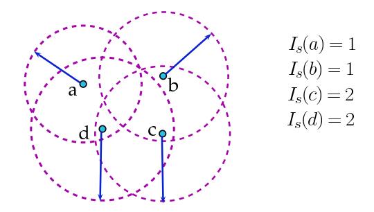
Figure 1. Sample of four nodes with their corresponding Sender interference.
Figure 1 shows a network with four nodes with their corresponding Sender interference values. Bilo and Proietti [3] proposed an algorithm for minimizing the maximum ` Sender interference that gives an optimal solution and also studied the computational hardness of several minimization problems with some constraints on the connectivity predicate. Panda and Shetty [11] considered the two dimensional networks with sender centric model and proposed an algorithm for minimizing the maximum interference that gives an optimal solution. The authors also proposed a 2-factor approximation algorithm for minimizing the average interference. Agrawal and Das [1] proposed algorithms for minimizing the maximum interference and total interference of a network. For minimizing the total interference, the authors proposed an optimum algorithm of O(n) running time for the connectivity predicate Broadcast. Same authors proposed a heuristic for minimizing the total interference for strongly connected predicate case. Rangwala et al. [12] presented algorithms to construct network topologies for minimizing or approximately minimizing the maximum (or average) link (or nodal) interference of a network.
Liu and Mohapatra [8] studied the sensor placement problem in WSNs. The authors formulated the following problem: For a given required lifetime of a WSN along with initial energy at each sensor node and the number of sensor nodes, the objective is to determine how large an area this network can cover. They proposed a near-optimal greedy algorithm for this problem. Niati et al. [10] proposed a deployment scheme which enables the use of additional nodes in a WSN whenever required. This scheme deploys the spare nodes in the network to substitute the exhausted nodes. The authors presented the simulation results by considering a various number of spare nodes and studied the effect of the deployment in a WSN. Langetepe et al. [7] introduced a strategic deployment problem which aims to minimize the number of agents required to traverse the graph, subject to some particular conditions. Authors also proved that the problem of computing the optimal number of agents is NP-hard and gave an efficient, O(n log n) algorithm for trees and a 2-approximation (by Minimum Spanning Tree) algorithm for a general graph.
Deployment of vertices in an efficient way leads to a proper topology which optimizes the energy consumption of a given network. It is possible to reduce the interference by using the technique of deploying additional nodes at a suitable position. In the proposed algorithm, we make use of the same technique to reduce the interference of a given network. We deploy the additional nodes in the existing network so that the network remains connected and it minimizes the maximum Sender interference of the network. The idea of deploying additional nodes is motivated by the theoretical properties of Gabriel graphs. In this paper, we explore the properties of the Gabriel graph and try to minimize the maximum Sender interference of the given network. Rest of the paper is organized as follows: Section 2 explains the problem statement, section 3 presents the algorithm and its detailed explanation. Section 4 presents the results and analyzes it and finally, section 5 concludes the paper.
2. Problem statement
For a given set V of n nodes, a weight function w and a set V ′ of additional nodes, the aim is to build a connected network T, with vertex set V ∪ V ′ that minimizes the maximum Sender interference of the network. The main idea is to reduce the Sender interference of the given network by deploying the additional nodes. The position of the n nodes will be the same but, the additional nodes are deployed to reduce the Sender interference. The above problem is formally defined as follows:
Problem: Minimizing Sender interference by Deployment of additional nodes.
Instance: A complete graph G = (V, E, w) where w : V × V → R + is weight function and set V ′ of additional nodes.
Objective: To construct a spanning tree T with vertex set V ∪ V ′ , that minimizes the maximum Sender interference.
3. Algorithm for minimizing the Sender interference
The idea of the algorithm: We have n nodes deployed on a Euclidean plane with a weight function w. Initially, we join each vertex with its nearest neighbor so that, each edge formed is Gabriel. Let
the induced spanning forest be T which consists of one or more connected components. Let the Euclidean MST of the graph be T1 which is also Gabriel. Every Gabriel graph has the Euclidean MST as its subgraph and it is obvious that T ⊂ T1. Now we assign Range to all the vertices in T as the distance to its farthest neighbor, as given in Eq. 1. Let E ′ be the set of all edges which are present in T1 but not in T, i.e., E ′ = {e ∈ T1 | e /∈ T}. At this step, we deploy the additional nodes at an appropriate location to reduce the maximum Sender interference without changing the position of the original nodes. An additional vertex u ∈ V ′ , is deployed at the bisection point of the edge e = pq ∈ E ′ , and half of the Euclidean distance between p and q is assigned as Range to the vertex u. Each time, an additional vertex is deployed only if there is a reduction in the maximum Sender interference of the network. We repeat this procedure for all the edges in E ′ . We present MSD (Minimizing Sender interference by Deployment of additional nodes) algorithm for the above formulated problem and given in Algorithm 1.
Algorithm 1: MSD
  Input: A complete graph G = (V, E, w) where w : V × V → R
                                                          + is weight function and set
         V
          ′ of additional nodes.
  Output: A spanning tree T with vertex set V ∪ V
                                              ′
                                              , with corresponding Range assignment
          R, minimizing the maximum Sender interference.
1 begin
2 Let IS(T) be the maximum Sender interference at any instance.
3 for each vertex v ∈ V do
4 Let v
             ′ be the nearest vertex to v
5 T = T ∪ {vv′}
6 R[v] = w(vv′
                     )
7 end
8 Let T1 be the Euclidean MST of the given set of nodes.
9 Let E
          ′ = {e | e ∈ T1 && e /∈ T}
10 for each edge e = vx ∈ E
                            ′ do
11 if deployment of an additional vertex u ∈ V
                                               ′
                                                , at the bisection point of e reduces the
         IS(T) then
12 T = T ∪ {vu, ux}
13 R[u] = w(vx)/2
14 E
              ′ = E
                   ′ \ {e}
15 end
16 end
17 for each vertex v ∈ V (T) do
18 Let u be the farthest adjacent vertex to v in T.
19 R[v] = w(uv)
20 end
21 return T, IS(T)
22 end
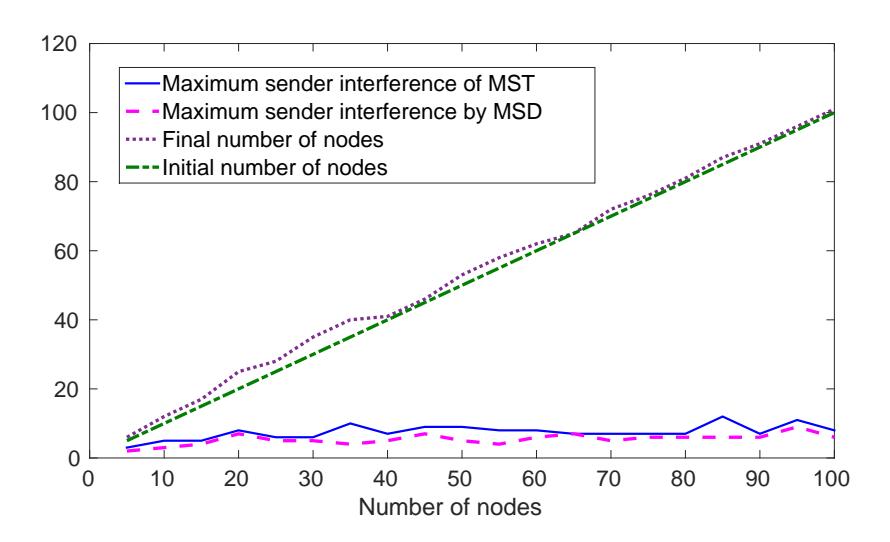
Figure 2. Illustration of Algorithm 1
Remark 3.1. The number of additional nodes to be deployed is not taken as an input, since the deployment of additional nodes may not always guarantee the reduction in the maximum Sender interference.
Example 3.1. In Figure 2, (a) shows a complete graph in which the Euclidean distance between every two nodes mentioned, (b) shows the spanning forest T formed by joining each vertex with its nearest vertex and (c) shows the Euclidean MST of the deployed nodes, denoted by T1, for the same set of vertices. For this graph, we have E ′ = {ad}, since ad is the only edge such that, ad ∈ T1 and ad /∈ T. So we require single additional vertex, as |E ′ | = 1, say V ′ = {f}. Now, if we place the new vertex f ∈ V ′ , at the bisection point of the edge ad and assign Range to f as w(ad)/2, then the resultant spanning tree is as shown in (d). The maximum Sender interference of the Euclidean MST is 3 but, after deploying the additional vertex f, it is reduced to 2. We see that the output is a spanning tree T with maximum Sender interference 2. The Range, Sender interference of each vertex in MST as well as the resultant spanning tree T obtained after the deployment of an additional vertex are reported in Table 1. We also observe that there is a decrease in the Range of vertices a and d after deploying the additional vertex f.
Theorem 3.2. Let V be the set of all nodes deployed on a Euclidean plane and S = {uv | uv is Gabriel edge for u, v ∈ V }. Then the graph T = (V, S) is always connected.
Proof. If possible, let us suppose that T is disconnected. Then there exist at least two connected components in T, say c1 and c2. Let the number of vertices in c1 and c2 be n1 and n2 respectively. Now, to establish the connectivity between these two components, we need to join them by an edge which does not belong to T. Totally, we have n1.n2 possible edges to join these two components. Let e be the edge with minimum value of w(e) among all the possible edges. Since it is the minimum among all the possible edges, the circle with edge e as its diameter does not have any other vertex in its interior. Therefore, the edge e is Gabriel but it does not belong to T, which
| T1 | T | |||
|---|---|---|---|---|
| Vertex | R(v) | IS(v) | R(v) | IS(v) |
| a | 4.6 | 2 | 3.6 | 2 |
| b | 3.6 | 1 | 3.6 | 1 |
| c | 1.7 | 1 | 1.7 | 1 |
| d | 4.6 | 3 | 2.3 | 2 |
| e | 1.7 | 2 | 1.7 | 2 |
| f | - | - | 2.3 | 2 |
Table 1. Range and Sender interference of each vertex of the graph shown in Figure 2.
contradicts the statement that T contains the set of all Gabriel edges of G. Hence, the set of all Gabriel edges of a complete graph forms a connected subgraph.
Theorem 3.3. [13] The graph formed by joining each vertex to its nearest vertex is acyclic.
Theorem 3.4. The graph formed by joining each vertex to its nearest vertex is always Gabriel.
Proof. Let T be the graph obtained by joining each vertex to its nearest vertex. If possible, let us suppose that T is not Gabriel, then there exists an edge uv in T which is not Gabriel. Since uv is not Gabriel, there exists a vertex x in the interior of the circle with u and v as the endpoints of its diameter. Then x is the nearest vertex to both u and v which contradicts the statement that u is the nearest vertex of v (or v is the nearest vertex of u). Therefore, each and every edge in T is Gabriel and thereby the graph formed by joining each vertex to its nearest vertex is always Gabriel.
Theorem 3.5. The Euclidean MST of a complete graph is always Gabriel.
Proof. From Theorem 3.2 it follows that every complete graph has a connected Gabriel graph as its subgraph. Every Gabriel graph has the Euclidean MST as its subgraph [9], which is also Gabriel. Therefore, the Euclidean MST of a complete graph is always Gabriel.
Theorem 3.6. [9] A tree with a vertex of degree greater than or equal to six is not Gabriel.
Corollary 3.1. The maximum degree of the Euclidean MST of a complete graph is less than 6.
Proof. If possible, let us suppose that the maximum degree of the Euclidean MST of a complete graph is greater than or equal to 6. Theorem 3.5 says that the Euclidean MST of a complete graph is always Gabriel. But, according to Theorem 3.6, if a tree has a vertex of degree greater than or equal to six, then it is not Gabriel. This is a contradiction to our assumption that the maximum degree of Euclidean MST is greater than or equal to 6.
Theorem 3.7. The algorithm MSD always results in a connected network.
Proof. MSD algorithm starts with the formation of a spanning forest T by joining each vertex with its nearest vertex. Next, it computes the Euclidean MST i.e., T1 which has exactly n−1 edges. We use E ′ , the set of all edges which belong to T1 but not to T, to establish the connectivity between the components in the spanning forest T. It is obvious that to achieve the connectivity in T, the set of edges in E ′ are sufficient enough. For each edge in e ∈ E ′ , we deploy an additional vertex from the set V ′ , at the bisection point of the edge and the Range assigned to that additional vertex is w(e)/2. Deployment is done only if there is a reduction in maximum Sender interference. For each edge in E ′ , either the edge is added to the resultant spanning tree (if there is no deployment) or it is bisected by an additional vertex which divides the existing edge into two edges. So, the connectivity is preserved in the resultant subgraph.
Theorem 3.8. The number of additional nodes required to be deployed in a network to minimize the maximum Sender interference is always bounded above by |E(T1)| − |E(T)|.
Proof. Let T be the spanning forest formed by connecting each vertex with its nearest vertex and |E(T)| be the number of edges in T. Let T1 be the Euclidean MST of the given set of vertices and |E(T1)| be the number of edges in T1. In the algorithm MSD, we consider E ′ i.e., the set of all edges present in T1 but not in T, for the deployment of the additional nodes. It is clear that |E ′ | = |E(T1)|−|E(T)|, whose value in worst case is n/2−1. So, the upper bound on the number of additional nodes to be deployed is |E(T1)| − |E(T)|.
Theorem 3.9. The algorithm MSD runs in O(n 2 ) time.
Proof. In the MSD algorithm, the formation of the spanning forest T takes O(n 2 ) running time. Computing Euclidean MST by Prim's algorithm [14] using the adjacency matrix takes O(n 2 ) running time. In worst case, T contains n/2 components as each vertex in T will be connected to at least one vertex. The set E ′ consisting of all edges present in T1 but not in T, contains at most (n−1)−(n/2) = (n/2)−1 edges. So, the for loop in step 10 of the algorithm takes O(n) running time. The set V ′ of additional nodes to be deployed has the cardinality n/2 at the most. The Range assignment to all the vertices of V in step 17 of the algorithm takes O(n 2 ) running time. Hence the algorithm is of O(n 2 ) running time.
4. Results
We deployed n number of vertices randomly (using rand() function which claims to be of uniform distribution) on a Euclidean plane of 1000×1000. The function w computes the Euclidean distance between each pair of vertices and an adjacency matrix is maintained whose entries are the weights as explained in section 1. We computed the Euclidean MST using Prim's algorithm and deployed the additional nodes in the network to reduce the maximum Sender interference further. We compared the maximum Sender interference of the MST and that of the resultant spanning tree obtained by the proposed algorithm after deploying the additional nodes.
Table 2 compares the maximum Sender interference of the MST of the considered complete graph and that of the spanning tree obtained by MSD algorithm after deployment of additional nodes. It shows the number of additional nodes required to be deployed in the network to reduce
Table 2. Maximum Sender interference of MST of and that of the resultant spanning tree T.
| Number of | Maximum Sender | Number of | Maximum Sender |
|---|---|---|---|
| initial nodes | T1 interference of | new nodes | T interference of |
| 5 | 3 | 1 | 2 |
| 10 | 5 | 2 | 3 |
| 15 | 5 | 2 | 3 |
| 20 | 8 | 2 | 6 |
| 25 | 6 | 3 | 3 |
| 30 | 6 | 1 | 5 |
| 35 | 10 | 1 | 4 |
| 40 | 12 | 1 | 8 |
| 45 | 9 | 1 | 7 |
| 50 | 9 | 3 | 5 |
| 55 | 8 | 3 | 4 |
| 60 | 8 | 2 | 6 |
| 65 | 7 | 5 | 5 |
| 70 | 7 | 2 | 5 |
| 75 | 7 | 1 | 6 |
| 80 | 7 | 1 | 6 |
| 85 | 12 | 2 | 6 |
| 90 | 7 | 1 | 6 |
| 95 | 11 | 1 | 9 |
| 100 | 8 | 1 | 6 |
Table 3. Average reduction and the decrease percentage of maximum Sender interference.
| Number | Average Sender interference | Decrease | ||
|---|---|---|---|---|
| of nodes | T1 | T | Difference | percentage |
| 10 | 5.6 | 4.5 | 1.1 | 19.64 |
| 20 | 6.7 | 5.0 | 1.7 | 25.37 |
| 30 | 7.0 | 4.5 | 2.5 | 35.71 |
| 40 | 6.6 | 5.2 | 1.4 | 21.21 |
| 50 | 7.0 | 5.4 | 1.6 | 22.85 |
| 60 | 7.5 | 5.5 | 2.0 | 26.66 |
| 70 | 7.3 | 5.7 | 1.6 | 21.91 |
| 80 | 8.5 | 6.1 | 2.4 | 28.23 |
| 90 | 8.0 | 5.7 | 2.3 | 28.75 |
| 100 | 8.1 | 6.1 | 2.0 | 24.69 |
| Number | Average Additional | Average reduction |
|---|---|---|
| of nodes | number of nodes | Sender interference |
| 10 | 1.5 | 2.3 |
| 20 | 1.2 | 2.6 |
| 30 | 1.2 | 2.9 |
| 40 | 1.4 | 3.4 |
| 50 | 1.2 | 3.9 |
| 60 | 1.5 | 4.0 |
| 70 | 1.5 | 4.1 |
| 80 | 1.6 | 4.0 |
| 90 | 1.2 | 4.0 |
| 100 | 1.3 | 4.7 |
Table 4. Average additional number of nodes and decrease percentage of the Sender interference.
the Sender interference. In Figure 3, we plotted the initial number of nodes, the final number of nodes after deployment and the maximum Sender interference of MST and that of the resultant spanning tree by MSD algorithm. Table 3 shows the average maximum Sender interference of the MST and that of the spanning tree obtained after deployment for which we ran the proposed algorithm 100 times for each value of n in order to establish the stability of the proposed algorithm. It also depicts the reduction percentage of the maximum Sender interference of the given network. Figure 4 indicates the average maximum Sender interference of MST and that of the resultant spanning tree by MSD algorithm for a various number of nodes.
Table 4 shows the average additional number of nodes and the average reduced maximum Sender interference after deploying the additional nodes. For each value of n, the algorithm was run 100 times. In Figure 5, the average additional number of nodes and average reduced Sender interference are plotted. Table 5 compares the total Range of the Euclidean MST with that of the spanning tree obtained after deployment and shows the difference. We observe that the total Range reduces after deployment most of the times. Although the increase in Range is found in few cases, it is significantly low. For computing the total Range, we used the function f(si , sj ) = t.dα [4], for two different nodes si and sj , where α is a constant related to path loss and t is the threshold value. In this experiment, we fix α = 2 and t = 1. Though the theoretical upper bound on the number of additional nodes is |E(T1)| − |E(T)|, the simulation results show that the maximum number of additional nodes deployed is 1.6 and the average reduction in the Sender interference is 4.7 for the networks of varying size.
5. Conclusion
In this paper, we proposed an algorithm for minimizing the maximum Sender interference of a WSN by deploying the additional nodes in the network. We explored the theoretical properties of Gabriel graphs to arrive at the proposed algorithm. The Sender interference of the Euclidean MST of the given set of nodes with that of the spanning tree obtained by proposed MSD algorithm
Table 5. Comparison of Range of MST and that of the spanning tree obtained by MSD.
| Number | Number of | Reduced | Range | Range | Difference |
|---|---|---|---|---|---|
| of nodes | new nodes | interference | of MST | by MSD | in Range |
| 10 | 1 | 3 | 2360.017 | 2124.214 | 235.803 |
| 15 | 1 | 4 | 2908.526 | 2694.510 | 214.016 |
| 20 | 1 | 3 | 4514.073 | 4515.457 | -1.384 |
| 25 | 1 | 1 | 4364.436 | 4359.812 | 4.624 |
| 30 | 1 | 6 | 3695.214 | 3599.839 | 95.375 |
| 35 | 1 | 5 | 5446.438 | 5307.238 | 139.2 |
| 40 | 2 | 4 | 5239.623 | 5126.469 | 113.154 |
| 45 | 1 | 4 | 5553.782 | 5466.333 | 87.449 |
| 50 | 1 | 3 | 6254.478 | 6196.371 | 58.107 |
| 55 | 1 | 5 | 6452.161 | 6363.571 | 88.59 |
| 60 | 1 | 3 | 6885.42 | 6766.571 | 118.849 |
| 65 | 1 | 2 | 6142.201 | 6166.646 | -24.445 |
| 70 | 1 | 3 | 7154.01 | 7029.977 | 124.033 |
| 75 | 1 | 9 | 7215.844 | 7194.791 | 21.053 |
| 80 | 1 | 3 | 7382.623 | 7350.221 | 32.402 |
| 85 | 2 | 2 | 7576.701 | 7485.605 | 91.096 |
| 90 | 2 | 5 | 8472.303 | 8365.898 | 106.405 |
| 95 | 1 | 3 | 7825.011 | 7756.247 | 68.764 |
| 100 | 1 | 7 | 8571.695 | 8480.457 | 91.238 |
| 200 | 1 | 4 | 11530.458 | 11468.851 | 61.607 |
| 300 | 1 | 4 | 14226.611 | 14180.234 | 46.377 |
| 400 | 1 | 4 | 16378.671 | 16352.799 | 25.872 |
| 500 | 1 | 3 | 18195.529 | 18191.765 | 3.764 |
| 600 | 1 | 3 | 20060.55 | 20038.535 | 22.015 |
| 700 | 2 | 2 | 21332.992 | 21285.335 | 47.657 |
| 800 | 1 | 3 | 22625.677 | 22604.13 | 21.547 |
| 900 | 1 | 3 | 24035.476 | 24008.373 | 27.103 |
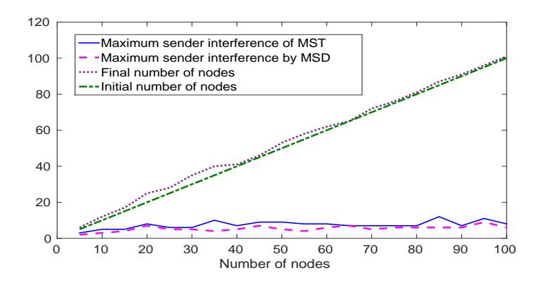
Figure 3. Maximum Sender interference of MST and the resultant spanning tree.
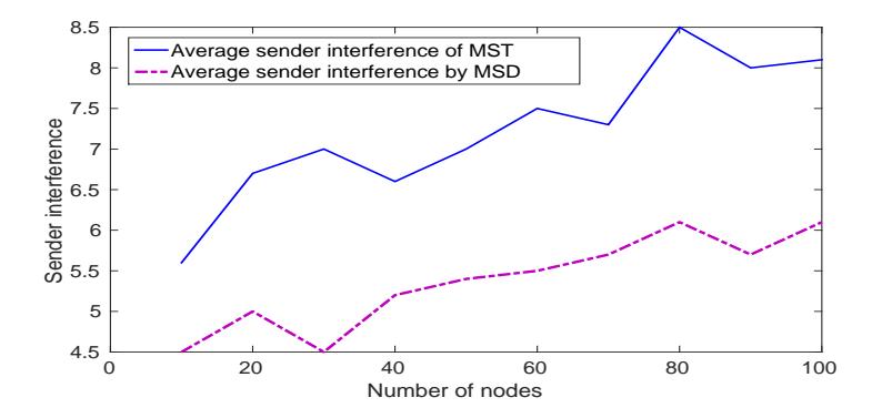
Figure 4. Average maximum Sender interference of MST and that of the resultant spanning tree.
are compared, through extensive simulation for a various number of nodes. We observed that the deployment of the additional nodes in the network reduces the maximum Sender interference of the network. The theoretical properties of the Gabriel graphs can be further explored for a study on interference in a WSN. Though the upper bound on the number of additional nodes is \(|E(T_1)| - |E(T)|\), the maximum number of additional nodes deployed is 1.6 and the maximum reduction in sender interference is 4.7 on an average. Simulation results also show that the average reduced Sender interference after deployment of additional nodes is 25.5 percentage. From the result, it is concluded that the number of additional nodes used does not increase as a function of n and the increase is by a small constant. It is also observed that as the number of nodes increases, the reduction in Sender interference also increases which demonstrates the scalability of the proposed algorithm.
Acknowledgement
The authors would like to acknowledge the National Institute of Technology Karnataka Surathkal, for the support in this research work.
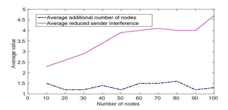
Figure 5. Average additional number of nodes and the average reduction in Sender interference.
References
- [1] P. Agrawal and G.K. Das, Improved interference in wireless sensor networks. Distributed Computing and Internet Technology, ICDCIT Proceedings, (2013), 92–102.
- [2] I.F. Akyildiz, W. Su, Y. Sankarasubramaniam, and E. Cayirci, Wireless sensor networks: a survey, Computer networks 38 (4) (2002), 393–422.
- [3] D. Bilò and G. Proietti, On the complexity of minimizing interference in ad-hoc and sensor networks. Theor. Comput. Sci., 402 (1) (2008), 43–55.
- [4] X. Cheng, B. Narahari, R. Simha, M.X. Cheng, and D. Liu, Strong minimum energy topology in wireless sensor networks: Np-completeness and heuristics. IEEE Trans. Mob. Comput., 2 (3) (2003), 248–256.
- [5] K.R. Gabriel and R.R. Sokal, A new statistical approach to geographic variation analysis, Systematic Biology, 18 (3) (1969), 259–278.
- [6] R. Hayward, D. Rappaport, and R. Wenger, Some extremal results on circles containing points. Discrete & Computational Geometry, 4 (3) (1989), 253–258.
- [7] E. Langetepe, A. Lenerz, and B. Brüggemann (2014). Strategic deployment in graphs. Informatica (Slovenia), 39 (3) (2015), 237–247.
- [8] X. Liu and P. Mohapatra, Placement of sensor nodes in wireless sensor networks. (2004)
- [9] D.W. Matula and R.R. Sokal, Properties of gabriel graphs relevant to geographic variation research and the clustering of points in the plane. Geographical analysis, 12 (3) (1980), 205–222.
- [10] R. Niati, N. Yazdani, and M. Nourani, Deployment of spare nodes in wireless sensor networks. Wireless and Optical Communications Networks, IFIP Conference proceedings, IEEE, (2006), 5-pp.
- [11] B. Panda and D.P. Shetty, Strong minimum interference topology for wireless sensor networks, Advanced Computing, Networking and Security, Springer, 7135 (2011), 366–374.
- [12] S. Rangwala, R. Gummadi, R. Govindan, and K. Psounis, Interference aware fair rate control in wireless sensor networks, ACM SIGCOMM Conference Proceedings, 36 (4) (2006), 63–74.
- [13] D.P. Shetty, M.P. Lakshmi, Algorithms for minimizing the receiver interference in a wireless sensor network. DISCOVER conference proceedings, IEEE, (2016), 113–118.
- [14] D.B. West, Introduction to graph theory, Pearson Education (Singapore) Pte.Ltd., Second Edition, 2001.