Sushobhan Maity, A. K. Bhuniya

Department of Mathematics, Visva-Bharati, Santiniketan-731235, India

susbhnmaity@gmail.com, anjankbhuniya@gmail.com

In this article, we introduce and characterize linear dependence graph Γ(V ) of a finite dimensional vector space V over a finite field of q elements. Two vector spaces U and V are isomorphic if and only if their linear dependence graphs Γ(U) and Γ(V ) are isomorphic. The linear dependence graph Γ(V ) is Eulerian if and only if q is odd. Highly symmetric nature of Γ(V ) is reflected in its automorphism group S^m ⊕ (⊕^{m i}=1Sq−1), where m = q ⁿ−1 q−1 . Besides these basic characterizations of Γ(V ), the main contribution of this article is to find eigen values of adjacency matrix, Laplacian matrix and distance matrix of this graph.

Keywords: graph, linear dependence, Laplacian, distance, spectrum Mathematics Subject Classification : 05C25, 05C50, 05C69

DOI: 10.5614/ejgta.2019.7.1.4

1. Introduction

The study of different algebraic structures, using the properties of graphs associated to them, has become an exciting topic of research in the last three decades. This new technique of studying algebraic structures leads to many fascinating results and questions. For various constructions of graphs on different algebras we refer to [2, 7] on rings, [3, 5] on groups, [6] on semigroups, [23, 24, 26, 33] on posets, [9, 10, 11, 12] on vector spaces.

Received: 26 October 2017, Revised: 13 June 2018, Accepted: 24 December 2018.

A field F is called finite if it contains only finitely many elements. We call a vector space V finite dimensional if it has a finite basis. We denote the null vector of V by \(\theta\) and \(V^* = V \setminus \{\theta\}\). Throughout this article, unless stated otherwise, F stands for a field of q elements and V stands for a finite dimensional vector space over F of dimension n. Hence the vector space V has \(q^n\) elements. We associate a simple graph \(\Gamma(V)\) to a vector space V with vertex set V, and two distinct vertices \(u,v\in V\) are adjacent if and only if u and v are linearly dependent in V. We call the graph \(\Gamma(V)\) the linear dependence graph of V.

The main objective of this paper is to study the interplay of linear algebraic properties of V and graph theoretic properties of \(\Gamma(V)\). Here we prove that two vector spaces U and V are isomorphic if and only if \(\Gamma(U)\) and \(\Gamma(V)\) are isomorphic as graphs. As a consequence, it follows that the invariants of the graph \(\Gamma(V)\) remains invariant algebraically on V. For example, the adjacency spectrum, Laplacian spectrum and distance spectrum of \(\Gamma(V)\) remains invariant up to isomorphism of vector spaces. Thus the results on \(\Gamma(V)\) help illuminate properties of V.

We will include basic definitions of graph theory as needed. Basic references for graph theory are [4, 35]; for vector spaces, see [21]. Now we recall some notions of graph theory and vector spaces, which have been used here commonly. In this article, every graph is simple. Let G =\((\mathbb{V},\mathbb{E})\) be a graph. The number of vertices in \(\mathbb{V}\) is called the order of G. A graph \(G'=(\mathbb{V}',\mathbb{E}')\)is called a subgraph of \(G = (\mathbb{V}, \mathbb{E})\) if \(\mathbb{V}' \subseteq \mathbb{V}\) and \(\mathbb{E}' \subseteq \mathbb{E}\). For any vertex \(v \in \mathbb{V}\), the number of edges incident with v is called the degree of v; which we denote by deg(v). For two distinct vertices \(a, b \in \mathbb{V}\), \(a \sim b\) means that a, b are adjacent. If \(a \sim b\) for every pair of distinct vertices \(a,b \in \mathbb{V}\), then G is called a complete graph. A path of length k in G is an alternating sequence of vertices and edges \(v_0e_0v_1e_1v_2\cdots v_{k-1}e_{k-1}v_k\), where \(v_i\)'s are distinct (except possibly \(v_0\) and \(v_k\)) and \(e_i\) is the edge joining \(v_i\) and \(v_{i+1}\). A cycle is a path with the initial and the terminal vertices same. If there is a path between any pair of distinct vertices of G, then it is called a connected graph. For any two distinct vertices \(u, v \in \mathbb{V}\), the distance d(u, v) of u and v is defined as the length of the shortest path between u and v. Let \(G = (\mathbb{V}, \mathbb{E})\) and \(G' = (\mathbb{V}', \mathbb{E}')\) be two graphs. A mapping \(\phi: \mathbb{V} \longrightarrow \mathbb{V}'\) is called a homomorphism if for every \(a, b \in \mathbb{V}\), \(a \sim b\) in G implies that \(\phi(a) \sim \phi(b)\) in G'. A bijective mapping \(\phi: \mathbb{V} \longrightarrow \mathbb{V}'\) is called an isomorphism if both \(\phi\) and \(\phi^{-1}\) are homomorphisms. Thus a bijective mapping \(\phi: \mathbb{V} \longrightarrow \mathbb{V}'\) is an isomorphism if for every \(a, b \in \mathbb{V}\), \(a \sim b\) in G if and only if \(\phi(a) \sim \phi(b)\) in G'.

For any \(m \times m\) square matrix B, we denote the determinant of B by \(\det B\) or |B|; and the characteristic polynomial \(\det(xI_m - B)\) by \(\Theta(B, x)\). As usual, we denote the ring of all integers modulo m by \(\mathbb{Z}_m\). To avoid trivialities, we assume that \(\dim(V) \geqslant 1\).

The organization of this article is as follows. In addition to this introduction, this article comprises of two sections. Section 2 studies some basic properties of \(\Gamma(V)\) like connectedness, completeness, planarity, etc. Also several graph theoretic parameters including independence number, domination number, chromatic number are found there. Also we find the automorphism group of \(\Gamma(V)\); and a necessary and sufficient condition for \(\Gamma(V)\) to be Eulerian in this section. Section 3 considers the adjacency matrix, Laplacian matrix and distance matrix of the graph. We find eigen values of these three matrices associated with \(\Gamma(V)\), and hence the graph-spectrum based parameters of \(\Gamma(V)\), like algebraic connectivity, energy, etc.

2. Properties of \(\Gamma(V)\)

In this section, we characterize some basic properties of \(\Gamma(V)\) like connectedness, completeness, planarity; and find parameters like clique number, chromatic number, etc. Also we find the group of all automorphisms on \(\Gamma(V)\).

The null vector \(\theta\) is adjacent to every other vertices in \(\Gamma(V)\). Hence \(\Gamma(V)\) is a connected graph for every vector space V. Now we give an example to show the typical form of the linear dependence graph \(\Gamma(V)\) of V.

Let \(\mathbb{Z}_2\) be the ring of all integers modulo 2. Then the polynomial \(x^2 + x + 1\) is irreducible over \(\mathbb{Z}_2\), and so \(F = \mathbb{Z}_2/\langle x^2 + x + 1 \rangle\) is a field of four elements. Consider a vector space V of dimension n over F. Then the linear dependence graph \(\Gamma(V)\) of V is as follows:

Figure 1. The linear dependence graph of a vector space over \(F = \mathbb{Z}_2/\langle x^2 + x + 1 \rangle\).

Thus we see that the graph \(\Gamma(V)\) can not be complete if dim V>1. In fact we have:

Theorem 2.1. \(\Gamma(V)\) is complete if and only if n=1.

Proof. Let \(a \in V\) be a non-null vector. Since \(\Gamma(V)\) is complete for every \(b \in V\), \(b = \lambda a\) for some \(\lambda \in F\). Thus \(V = \langle a \rangle = \{\lambda a : \lambda \in F\}\), showing dim(V) = 1.

Converse is trivial.

The number of edges of a graph is called the size of G.

Theorem 2.2. The size m of \(\Gamma(V)\) is \(\frac{q(q^n-1)}{2}\).

Proof. The null vector \(\theta\) is adjacent with every non-null vector of V. Since \(|V|=q^n\), so degree of the vertex \(\theta\) is \(q^n-1\). Let \(a\neq \theta\) be a vertex of \(\Gamma(V)\). Then a vertex \(b\in \Gamma(V)\) is adjacent with a if and only if \(b\neq a\) and \(b=\lambda a\) for some \(\lambda\in F\). Since |F|=q, so degree of each of the non-zero vector is q-1. Hence \(2m=q^n-1+(q^n-1)(q-1)\) and it follows that \(m=\frac{q(q^n-1)}{2}\).

The diameter of a graph \(G=(\mathbb{V},\mathbb{E})\) is defined as \(diam(G)=max_{u,v\in\mathbb{V}}d(u,v)\), if it exists. Otherwise, diam(G) is defined as \(\infty\). Since the null vector \(\theta\) is adjacent with every other vertices of \(\Gamma(V)\), we have the following result.

Theorem 2.3. \(\Gamma(V)\) is connected and \(diam(\Gamma(V)) = 2\).

A subset D of \(\mathbb{V}\) in a graph \(G = (\mathbb{V}, \mathbb{E})\) is called a dominating set if each element of \(\mathbb{V} \setminus D\) is adjacent to at least one element of D. If no proper subset of D is a dominating set for G, then D is called a minimal dominating set for G. The size of the smallest dominating set is called the domination number of G.

Since \(\theta\) is adjacent to every other vertices in \(\Gamma(V)\), it follows that \(\{\theta\}\) is the smallest dominating subset of V. Thus we have the following result.

Theorem 2.4. The domination number of \(\Gamma(V)\) is 1.

A subset I of \(\mathbb{V}\) in a graph \(G=(\mathbb{V},\mathbb{E})\) is said to be independent if no two elements of I are adjacent. The size of the largest independent set is called the independence number of G.

Note that the number of 1-dimensional subspaces of V is \(\frac{q^{n}-1}{q-1}=q^{n-1}+q^{n-2}+\cdots+1\).

Theorem 2.5. The independence number of \(\Gamma(V)\) is \(q^{n-1} + q^{n-2} + \cdots + 1\).

Proof. It is easy to see that a subset I of V consists of a representatives from each of the 1-dimensional subspaces of V, is a maximal independent set. Then \(|I| = q^{n-1} + q^{n-2} + \cdots + 1\). If possible, suppose that there exists an independent set I' of cardinality greater than \(q^{n-1} + q^{n-2} + \cdots + 1\). Since total number of 1-dimensional subspaces of V is \(q^{n-1} + q^{n-2} + \cdots + 1\), so it follows that there are at least two elements \(a, b \in I'\) such that a, b are in a same 1-dimensional subspace of V. Then \(a \sim b\), which contradicts that I' is independent. Thus the independence number of \(\Gamma(V)\) is \(q^{n-1} + q^{n-2} + \cdots + 1\).

Two graphs \(G = (\mathbb{V}, \mathbb{E})\) and \(G' = (\mathbb{V}', \mathbb{E}')\) are said to be isomorphic if there is an isomorphism \(\phi : \mathbb{V} \longrightarrow \mathbb{V}'\).

Theorem 2.6. Two vector spaces V and W are isomorphic if and only if their corresponding graphs \(\Gamma(V)\) and \(\Gamma(W)\) are isomorphic.

Proof. Let V and W be isomorphic. Then there exists a vector space isomorphism \(T:V\to W\). If \(\alpha\sim\beta\) in \(\Gamma(V)\), then \(\alpha=\lambda\beta\) for some \(\lambda\in F\) and so \(T(\alpha)=\lambda T(\beta)\). Thus \(T(\alpha)\sim T(\beta)\) in \(\Gamma(W)\). Since T is an isomorphism, similarly \(T(\alpha)\sim T(\beta)\) in \(\Gamma(W)\) implies that \(\alpha\sim\beta\) in \(\Gamma(V)\). Hence \(\Gamma(V)\) and \(\Gamma(W)\) are isomorphic as graphs.

Conversely, let \(\phi: \Gamma(V) \to \Gamma(W)\) be a graph isomorphism. Let dimV = m and dimW = n. Since the independence numbers of two isomorphic graphs are the same, so we have \(q^{m-1} + q^{m-2} + \cdots + 1 = q^{n-1} + q^{n-2} + \cdots + 1\) and so m = n. Hence the vector spaces V and W are isomorphic. \(\Box\)

A clique in a graph \(G = (\mathbb{V}, \mathbb{E})\) is a complete subgraph of G. The size of the largest clique is called the clique number of G and is denoted by \(\omega(G)\).

Theorem 2.7. Let M be a clique of \(\Gamma(V)\), then M is maximal if and only if M is an 1-dimensional subspace of V. Hence the clique number \(\omega(\Gamma(V))\) of \(\Gamma(V)\) is q.

Proof. Let M be a maximal clique of Γ(V ). Since θ is adjacent with every other vertices of Γ(V ), there exists x 6= {θ} such that θ, x ∈ M. Since M is maximal, < x >= {λx|λ ∈ F} ⊆ M. Now, let z ∈ M. Then z ∼ x implies that z = λx for some λ ∈ F and so z ∈< x >. Hence M =< x > for some x ∈ V ∗ , showing that M is an 1-dimensional subspace of V .

Converse is trivial.

The chromatic number of a graph G = (V, E), written as χ(G), is the minimum number of colours needed for labeling the vertices in V so that adjacent vertices get different colours.

Theorem 2.8. Chromatic number of Γ(V ) is q.

Proof. If two vectors a and b are adjacent in Γ(V ), then they are in a same 1-dimensional subspace of V . Now |F| = q implies that an 1-dimensional subspace of V contains q elements. Hence the chromatic number χ(Γ(V )) ≤ q. Also χ(Γ(V )) ≥ ω(Γ(V )) = q. Hence χ(Γ(V )) = q.

A graph G = (V, E) is said to be Eulerian if it contains a cycle consisting of all the edges of G exactly once.

Lemma 2.1. The linear dependence graph Γ(V ) is Eulerian if and only if q is odd.

Proof. If q is an odd positive integer, then from the proof of the Theorem 2.2, we see that the degree of every vertex of Γ(V ) is an even integer. Hence the graph Γ(V ) is Eulerian.

Conversely, assume that Γ(V ) is Eulerian. Then degree of every vertices is even. Hence for every v ∈ V ∗ , deg(v) = q − 1 implies that q is odd.

An edge cutset in a graph G = (V, E) is a subset X of edges such that deletion of the edges in X increases the number of connected components of G. If G is connected, then the edge connectivity of G is the minimum number of edges in an edge cutset.

Theorem 2.9. Edge connectivity of Γ(V ) is q − 1.

Proof. From Theorem 2.3, we have the diameter of Γ(V ) is 2. So, the edge connectivity of Γ(V ) is equal to its minimum degree, i.e. q − 1 (Theorem 6; [25]).

A vertex cutset in a graph G = (V, E) is a subset Y of vertex such that deletion of the vertices in Y increases the number of connected components of G. If G is connected, then the vertex connectivity of G is the minimum number of vertices in a vertex cutset.

Deletion of the vertex θ makes the graph Γ(V ) disconnected. Hence we have the following result.

Theorem 2.10. The vertex connectivity of the graph Γ(V ) is 1.

A graph G = (V, E) is called planer if it can be drawn on a plane such that no two edges intersect at a point other than their common vertex. A graph G = (V, E) is called bipartite if the vertices can be partitioned into two classes such that every edge has one end in a class and other end in another class. If moreover, every two vertices from different classes are adjacent, then G is called complete bipartite. A complete bipartite graph with m and l vertices in two classes is denoted by Km,l. We denote a complete graph of m vertices by Km. The famous Kuratowski's Theorem states that a graph G is planer if and only if it does not contain any subgraph isomorphic to K⁵ or K3,3.

Theorem 2.11. \(\Gamma(V)\) is planar if and only if q = 2, 3, 4.

Proof. Every 1-dimensional subspace of V is a complete subgraph of \(\Gamma(V)\). So, for \(q \geq 5\), \(\Gamma(V)\) contains \(K_5\), the complete subgraph of \(\Gamma(V)\) of five vertices, which is nonplanar. Rest of the result follows from Figure 1 and the following.

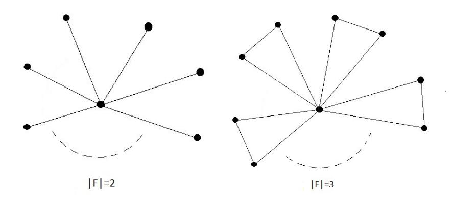
Figure 2. Examples of linear dependence graphs when |F| = 2, 3.

An automorphism on a graph \(G = (\mathbb{V}, \mathbb{E})\) is an isomorphism \(\phi : \mathbb{V} \longrightarrow \mathbb{V}\). It is well-known that that the set of all automorphisms on G is a group which we denote by Aut(G). The group Aut(G) is used to study symmetry of the graph G.

Theorem 2.12. Let F be a finite field of order q and V be a vector space over F of dimension n. Then \(Aut(\Gamma(V)) \simeq S_m \oplus (\bigoplus_{i=1}^m S_{q-1})\), where \(m = q^{n-1} + \cdots + q + 1\).

Proof. In \(\Gamma(V)\), the maximal cliques are precisely the 1-dimensional subspaces of V and so contains q vertices. Since \(\theta\) is the only common element of the maximal cliques, it follows that the total number of maximal cliques is \(m=\frac{q^n-1}{q-1}=q^{n-1}+q^{n-2}+\cdots+q+1\). Let us denote these m maximal cliques by \(C_1,C_2,\cdots,C_m\) and \(C_i=\{\theta,v_1^i,v_2^i,\cdots,v_{q-1}^i\}\). Then for every \(1\leq i,j\leq m\), \(i\neq j\), we have \(C_i\cap C_j=\{\theta\}\).

Hence every graph automorphism \(f:\Gamma(V)\to\Gamma(V)\) induces a permutation \(\sigma_f\) on \(\{C_1,C_2,\cdots,C_m\}\). Also if \(\sigma_f(C_i)=C_j\), then we have a bijection \(f_i:\{v_1^i,v_2^i,\cdots,v_{q-1}^i\}\to\{v_1^j,v_2^j,\cdots,v_{q-1}^j\}\) and so a permutation \(\sigma_f^i\in S_{q-1}\). Thus we get a group isomorphism

\[f\longmapsto (\sigma_f,\sigma_f^1,\sigma_f^2,\cdots,\sigma_f^m)\] from \(Aut(\Gamma(V))\) onto \(S_m\oplus (\bigoplus_{i=1}^m S_{q-1}).\)

3. Spectrums of the graph \(\Gamma(V)\)

In this section, we find the eigen values of the adjacency matrix, Laplacian matrix and distance matrix of the graph \(\Gamma(V)\). Suppose that the vertices of a graph \(G = (\mathbb{V}, \mathbb{E})\) are labeled

Figure 3. The maximal cliques of Γ(V ).

v1, v2, · · · , vm. Then the adjacency matrix A(G) = (aij )m×^m of G is defined as follows:

\[a_{ij} = 1 \text{ if } v_i \sim v_j;\]
= 0 otherwise.

The notion of distance between two vertices of a graph G induces a matrix D(G) which we call the distance matrix of G. It is defined as follows: D(G) = (dij )m×^m where dij = d(vⁱ , v^j ). There is also another matrix of fundamental importance associated with every graph G, known as the Laplacian matrix of G and defined by L(G) = D(G) − A(G), where D(G) is the diagonal matrix of vertex degrees. From the definition it follows that all these three matrices associated with a graph G are symmetric. The Laplacian matrix is positive semidefinite and singular with 0 as the smallest eigenvalue. The eigen values of the adjacency matrix, the Laplacian matrix and the distance matrix are known as the adjacency spectrum, the Laplacian spectrum and the distance spectrum of the graph G respectively. These spectrums play an important role in the study of many graph theoretic properties like connectivity, colouring, energy of a graph, number of spanning trees, Estrada index, etc. We refer to [19, 22] and [32] for more results and applications of these three spectrums.

Let v1, v2, · · · , vⁿ be the n-vertices of a graph G. Then A^v1,v2,··· ,v^k (G) is defined as the principal submatrix of A(G) formed by deleting the rows and columns corresponding to the vertices v1, v2, · · · , vk. In particular if k = |G|, then we define Θ(A^v1,v2,··· ,v|G^| (G), x) = 1.

The field F contains q elements and dim^F V = n implies that V has exactly q ⁿ−¹ + · · · + q + 1 number of 1-dimensional subspaces and each of these 1-dimensional subspaces contains exactly q − 1 nonzero vectors. Also note that no nonzero vector of V can belong to more than one 1 dimensional subspace. We label the vertices of Γ(V ) as follows: take θ first, then the nonzero vectors belonging to a 1-dimensional subspace successively and so on. Since every 1-dimensional

subspace is a clique and no two nonzero vectors from two different 1-dimensional subspaces are adjacent, the adjacency matrix \(A(\Gamma(V))\) of \(\Gamma(V)\) is as follows:

\[\text{[rumus tidak dapat ditampilkan dengan baik — lihat PDF asli]}\]

Order of this matrix is \(q^n\). Hence \(A_{\theta}(\Gamma(V))\) is a matrix of order \(q^n-1\). Also \(A_{\theta}(\Gamma(V))\) is a block diagonal matrix, having \(q^{n-1}+q^{n-2}+\cdots+q+1\) diagonal blocks \(J_{q-1}-I_{q-1}\), where \(J_{q-1}\) is the square matrix of order q-1 such that each entry is 1 and \(I_{q-1}\) is the identity matrix of order q-1.

The degree of the null vector is \(q^n-1\) and the degree of all other elements is q-1. Hence the Laplacian matrix of \(\Gamma(V)\) is

\[\text{[rumus tidak dapat ditampilkan dengan baik — lihat PDF asli]}\]

The distance between any two vertices of an 1-dimensional subspace is 1 and is 2 if they belong to two distinct 1-dimensional subspaces of V. So the distance matrix of \(\Gamma(V)\) is

\[\text{[rumus tidak dapat ditampilkan dengan baik — lihat PDF asli]}\]

Hence we have the following results.

Theorem 3.1. The characteristic polynomial of the adjacency matrix of \(\Gamma(V)\) is

\[\Theta(A(\Gamma(V)), x) = \{x^2 - (q-2)x - (q^n - 1)\}\{x - (q-2)\}^{q^{n-1} + \dots + q}(x+1)^{(q-2)(q^{n-1} + \dots + 1)}.\]

Proof. The characteristic polynomial of \(A(\Gamma(V))\) is

\[\Theta(A(\Gamma(V)), x) = \begin{vmatrix} x & -1 & -1 & \cdots & -1 & \cdots & -1 & -1 & \cdots & -1 \\ -1 & x & -1 & \cdots & -1 & \cdots & 0 & 0 & \cdots & 0 \\ -1 & -1 & x & \cdots & -1 & \cdots & 0 & 0 & \cdots & 0 \\ \vdots & \vdots & \vdots & \ddots & \vdots & \vdots & \vdots & \vdots & \vdots \\ -1 & -1 & -1 & \cdots & x & \cdots & 0 & 0 & \cdots & 0 \\ \vdots & \vdots & \vdots & \vdots & \vdots & \ddots & \vdots & \vdots & \vdots & \vdots \\ -1 & 0 & 0 & \cdots & 0 & \cdots & x & -1 & \cdots & -1 \\ -1 & 0 & 0 & \cdots & 0 & \cdots & -1 & x & \cdots & -1 \\ \vdots & \vdots & \vdots & \ddots & \vdots & \vdots & \vdots & \vdots & \ddots & \vdots \\ -1 & 0 & 0 & \cdots & 0 & \cdots & -1 & -1 & \cdots & x \end{vmatrix}\]

Multiply the 1st row by (x-(q-2)) and apply the row operation \(R_1'=R_1+R_2+\cdots+R_{q^n}\). Then expanding the determinant in terms of the first row, we get

\[\Theta(A(\Gamma(V)), x) = \frac{\{x^2 - (q-2)x - (q^n - 1)\}}{x - (q-2)} \cdot \begin{vmatrix} x & -1 & \cdots & -1 \\ -1 & x & \cdots & -1 \\ \vdots & \vdots & \ddots & \vdots \\ -1 & -1 & \cdots & x \end{vmatrix}_{(q-1) \times (q-1)}^{q^{n-1} + q^{n-2} + \cdots + q + 1}\]

Let

\[A_{1} = \begin{vmatrix} x & -1 & \cdots & -1 \\ -1 & x & \cdots & -1 \\ \vdots & \vdots & \ddots & \vdots \\ -1 & -1 & \cdots & x \end{vmatrix}_{(q-1)\times(q-1)}\] (1)

Multiply the 1st row of (1), by (x - (q - 3)) and apply the row operation by \(R'_1 = R_1 + R_2 + \cdots + R_{q-1}\). Then expanding the determinant in terms of the first row, we get

\[A_{1} = \frac{(x+1)(x-(q-2))}{x-(q-3)} \cdot \begin{vmatrix} x & -1 & \cdots & -1 \\ -1 & x & \cdots & -1 \\ \vdots & \vdots & \ddots & \vdots \\ -1 & -1 & \cdots & x \end{vmatrix}_{(q-2)\times(q-2)}\]

Again multiply the 1st row by (x - (q - 4)) and then apply the row operation \(R'_1 = R_1 + R_2 + \cdots + R_{q-2}\). Then expanding in terms of 1st row, we get

\[A_{1} = \frac{(x+1)^{2}(x-(q-2))}{x-(q-4)} \cdot \begin{vmatrix} x & -1 & \cdots & -1 \\ -1 & x & \cdots & -1 \\ \vdots & \vdots & \ddots & \vdots \\ -1 & -1 & \cdots & x \end{vmatrix}_{(q-3)\times(q-3)}\]

Continuing in this way, we get \(A_1 = (x+1)^{q-2}(x-(q-2))\) and so,

\[\begin{split} \Theta(A(\Gamma(V)),x) = & \frac{\{x^2 - (q-2)x - (q^n-1)\}}{\{x - (q-2)\}} \{(x - (q-2)\}^{q^{n-1} + \dots + 1} (x+1)^{(q-2)(q^{n-1} + \dots + 1)} \\ = & \{x^2 - (q-2)x - (q^n-1)\} \{x - (q-2)\}^{q^{n-1} + \dots + q} (x+1)^{(q-2)(q^{n-1} + \dots + 1)}. \end{split}\]

Let \(G=(\mathbb{V},\mathbb{E})\) be a graph of m vertices. Suppose that the m eigen values of the adjacency matrix A(G) of G are \(\lambda_1,\lambda_2,\cdots,\lambda_m\). Then the energy of the graph G, denoted by \(\varepsilon(G)\), is defined to be \(\sum_{i=1}^n |\lambda_i|\). Recently, Ernesto Estrada [15] has introduced a graph-spectrum based invariant defined as

\[EE(G) = \sum_{i=1}^{m} e^{\lambda_i}.\]

Now it is known as the Estrada index of the graph G. Though it has been introduced only in 2000, already it has been found significant applications in different uncorrelated fields like biochemistry, physical chemistry, network theory, information theory, etc [20]. Also a large number of articles are devoted to study of its mathematical properties [8, 13, 14, 27, 28, 29, 30, 31, 34].

Thus from Theorem 3.1, we have the following consequences:

Corollary 3.1. The energy of the graph \(\Gamma(V)\) is \(2(q-2)(q^{n-1}+\cdots+1)\).

Corollary 3.2. The Estrada index on \(\Gamma(V)\) is given by:

\[2e^{\frac{q-2}{2}}\cosh(\frac{\sqrt{4q^n+q^2-4q}}{2}) + e^{q-2}(q^{n-1}+\cdots+q) + (q-2)(q^{n-1}+\cdots+1)e^{-1}.\]

Theorem 3.2. The characteristic polynomial of the Laplacian matrix of \(\Gamma(V)\) is

\[\Theta(L(\Gamma(V)), x) = x(x - q^n)(x - 1)^{q^{n-1} + \dots + q}(x - q)^{(q-2)(q^{n-1} + \dots + 1)}.\]

Proof. The characteristic polynomial of \(L(\Gamma(V))\) is

\[\Theta(L(\Gamma(V)), x) = \begin{bmatrix} x - (q^n - 1) & 1 & \cdots & 1 & \cdots & 1 & \cdots & 1 \\ 1 & x - (q - 1) & \cdots & 1 & \cdots & 0 & \cdots & 0 \\ \vdots & \vdots & \ddots & \vdots & \vdots & \vdots & \ddots & \vdots \\ 1 & 1 & \cdots & x - (q - 1) & \cdots & 0 & \cdots & 0 \\ \vdots & \vdots & \vdots & \vdots & \ddots & \vdots & \vdots & \vdots \\ 1 & 0 & \cdots & 0 & \cdots & x - (q - 1) & \cdots & 1 \\ \vdots & \vdots & \ddots & \vdots & \vdots & \vdots & \ddots & \vdots \\ 1 & 0 & \cdots & 0 & \cdots & 1 & \cdots & x - (q - 1) \end{bmatrix}\]

Applying the row operation \(R'_1 = R_1 + R_2 + \cdots + R_{q^n}\), we get

\[\Theta(L(\Gamma(V)),x) = x \cdot \begin{vmatrix} 1 & 1 & \cdots & 1 & \cdots & 1 & \cdots & 1 \\ 1 & x - (q-1) & \cdots & 1 & \cdots & 0 & \cdots & 0 \\ \vdots & \vdots & \ddots & \vdots & \vdots & \vdots & \ddots & \vdots \\ 1 & 1 & \cdots & x - (q-1) & \cdots & 0 & \cdots & 0 \\ \vdots & \vdots & \vdots & \vdots & \ddots & \vdots & \vdots & \vdots \\ 1 & 0 & \cdots & 0 & \cdots & x - (q-1) & \cdots & 1 \\ \vdots & \vdots & \ddots & \vdots & \vdots & \vdots & \vdots & \vdots \\ 1 & 0 & \cdots & 0 & \cdots & x - (q-1) & \cdots & 1 \end{vmatrix}\]

Multiply the 1st row by (x-1) and then apply the row operation \(R_1' = R_1 - R_2 - \cdots - R_{q^n}\). Then expanding the determinant in terms of the first row, we get

\[\Theta(L(\Gamma(V)), x) = \frac{x(x-q^n)}{(x-1)} \cdot \begin{vmatrix} x - (q-1) & 1 & \cdots & 1 \\ 1 & x - (q-1) & \cdots & 1 \\ \vdots & \vdots & \ddots & \vdots \\ 1 & 1 & \cdots & x - (q-1) \end{vmatrix}_{(q-1) \times (q-1)}^{q^{n-1} + q^{n-2} + \cdots + q + 1}\]

Let

\[L_{1} = \begin{vmatrix} x - (q-1) & 1 & \cdots & 1 \\ 1 & x - (q-1) & \cdots & 1 \\ \vdots & \vdots & \ddots & \vdots \\ 1 & 1 & \cdots & x - (q-1) \end{vmatrix}_{(q-1) \times (q-1)}\] (2)

Multiply the 1st row of (2), by (x-2) and apply the row operation by \(R'_1 = R_1 - R_2 - \cdots - R_{q-1}\). Then expanding the determinant in terms of the first row, we get

\[L_{1} = \frac{(x-1)(x-q)}{(x-2)} \cdot \begin{vmatrix} x - (q-1) & 1 & \cdots & 1 \\ 1 & x - (q-1) & \cdots & 1 \\ \vdots & \vdots & \ddots & \vdots \\ 1 & 1 & \cdots & x - (q-1) \end{vmatrix}_{(q-2)\times(q-2)}\]

Again multiply the 1st row by (x-3) and then apply the row operation \(R_1' = R_1 - R_2 - \cdots - R_{q-2}\). Then expanding in terms of 1st row, we get

\[L_{1} = \frac{(x-1)(x-q)^{2}}{(x-3)} \cdot \begin{vmatrix} x - (q-1) & 1 & \cdots & 1 \\ 1 & x - (q-1) & \cdots & 1 \\ \vdots & \vdots & \ddots & \vdots \\ 1 & 1 & \cdots & x - (q-1) \end{vmatrix}_{(q-3)\times(q-3)}\]

Continuing in this way, we get \(L_1 = (x-1)(x-q)^{q-2}\). So,

\[\Theta(L(\Gamma(V)), x) = \frac{x(x - q^n)}{(x - 1)} \cdot \{(x - 1)(x - q)^{q - 2}\}^{(q^{n - 1} + \dots + 1)}\]\[= x(x - q^n)(x - 1)^{q^{n - 1} + \dots + q}(x - q)^{(q - 2)(q^{n - 1} + \dots + 1)}.\]

The second smallest eigen value of the Laplacian matrix \(L(\Gamma)\) of a graph \(\Gamma\), is denoted by \(a(\Gamma)\). This quantity shares many properties with the vertex or edge-connectivity and according to Fiedler [16], is called the algebraic connectivity of \(\Gamma\). So, from Theorem 3.2, we have the following result.

Corollary 3.3. The algebraic connectivity of \(\Gamma(V)\) is 1.

Let \(G = (\mathbb{V}, \mathbb{E})\) be a graph of m vertices and l edges. Suppose that the m eigen values of the Laplacian matrix L(G) of G are \(\mu_1 \geqslant \mu_2 \geqslant \cdots \geqslant \mu_m = 0\). Recently Gutman et. al [19] have defined the Laplacian energy of the graph G as follows:

\[LE(G) = \sum_{i=1}^{m} |\mu_i - \frac{2l}{m}|.\]

Similar to Estrada index, Fath-Tabar et al. [17] introduced the Laplacian Estrada index as follows:

\[LEE(G) = \sum_{i=1}^{m} e^{\mu_i}.\]

Also, in the literature an alternative definition of Laplacian Estrada index is found [14]. However, we follow the definition of Fath-Tabar et al.

From Theorem 2.2 and Theorem 3.2, we have:

Corollary 3.4. (i) The Laplacian energy of the graph \(\Gamma(V)\) is

\[q^{n} + (\frac{q^{n}(q-1) - q}{q^{n}})(q^{n-1} + \dots + q) + (\frac{q}{q^{n}})(q-2)(q^{n-1} + \dots + 1).\]

(ii) The Laplacian Estrada index of \(\Gamma(V)\) is

\[1 + e^{q^n} + (q-2)(q^{n-1} + \dots + 1)e^q + (q^{n-1} + \dots + q)e.\]

A connected graph is called a tree if it has no cycle. A subgraph T of a connected graph G is called a spanning tree of G if T is a tree and contains all the vertices of G. The number of spanning trees of G, denoted by G, is equal to \(\frac{\mu_1\mu_2\cdots\mu_{n-1}}{n}\) [Theorem 4.11; [1]].

Thus from Theorem 3.2, we get

Corollary 3.5. The number of spanning trees of \(\Gamma(V)\) is \(q^{(q-2)(q^{n-1}+\cdots+1)}\).

Theorem 3.3. The characteristic polynomial of the distance matrix of \(\Gamma(V)\) is

\[\Theta(D(\Gamma(V)),x) = [x^2 - \{2(q^n-1) - q\}x - (q^n-1)](x+q)^{q^{n-1}+\dots+q}(x+1)^{(q-2)(q^{n-1}+\dots+1)}.\]

Proof. The characteristic polynomial of \(D(\Gamma(V))\) is

\[\Theta(D(\Gamma(V)),x) = \begin{vmatrix} x & -1 & -1 & \cdots & -1 & \cdots & -1 & -1 & \cdots & -1 \\ -1 & x & -1 & \cdots & -1 & \cdots & -2 & -2 & \cdots & -2 \\ -1 & -1 & x & \cdots & -1 & \cdots & -2 & -2 & \cdots & -2 \\ \vdots & \vdots & \vdots & \ddots & \vdots & \vdots & \vdots & \vdots & \ddots & \vdots \\ -1 & -1 & -1 & \cdots & x & \cdots & -2 & -2 & \cdots & -2 \\ \vdots & \vdots & \vdots & \vdots & \vdots & \ddots & \vdots & \vdots & \vdots & \vdots \\ -1 & -1 & -1 & \cdots & x & \cdots & -1 & x & \cdots & -1 \\ -1 & -2 & -2 & \cdots & -2 & \cdots & -1 & x & \cdots & -1 \\ \vdots & \vdots & \vdots & \ddots & \vdots & \vdots & \vdots & \vdots & \ddots & \vdots \\ -1 & -2 & -2 & \cdots & -2 & \cdots & -1 & -1 & \cdots & x \end{vmatrix}\]

Apply the successive column operations \(C'_i = C_i - 2C_1\) for \(i = 2, 3, \dots, q^n\); we get

\[\Theta(D(\Gamma(V)), x) = \begin{vmatrix} x & -1 - 2x & \cdots & -1 - 2x & \cdots & -1 - 2x & \cdots & -1 - 2x \\ -1 & x + 2 & \cdots & 1 & \cdots & 0 & \cdots & 0 \\ \vdots & \vdots & \ddots & \vdots & \vdots & \vdots & \ddots & \vdots \\ -1 & 1 & \cdots & x + 2 & \cdots & 0 & \cdots & 0 \\ \vdots & \vdots & \vdots & \vdots & \ddots & \vdots & \vdots & \vdots \\ -1 & 0 & \cdots & 0 & \cdots & x + 2 & \cdots & 1 \\ \vdots & \vdots & \ddots & \vdots & \vdots & \vdots & \ddots & \vdots \\ -1 & 0 & \cdots & 0 & \cdots & 1 & \cdots & x + 2 \end{vmatrix}\]

\[= (1+2x) \cdot \begin{vmatrix} \frac{x}{1+2x} & -1 & \cdots & -1 & \cdots & -1 & \cdots & -1 \\ -1 & x+2 & \cdots & 1 & \cdots & 0 & \cdots & 0 \\ \vdots & \vdots & \ddots & \vdots & \vdots & \vdots & \ddots & \vdots \\ -1 & 1 & \cdots & x+2 & \cdots & 0 & \cdots & 0 \\ \vdots & \vdots & \vdots & \vdots & \ddots & \vdots & \vdots & \vdots \\ -1 & 0 & \cdots & 0 & \cdots & x+2 & \cdots & 1 \\ \vdots & \vdots & \ddots & \vdots & \vdots & \vdots & \vdots & \vdots \\ -1 & 0 & \cdots & 0 & \cdots & 1 & \cdots & x+2 \end{vmatrix}\]

Multiply the 1st row by x+q and then apply the row operation \(R_1'=R_1+\cdots+R_{q^n}\), we get

\[\Theta(D(\Gamma(V)), x) = \frac{[x^2 - \{2(q^n - 1) - q\}x - (q^n - 1)]}{(x + q)} \cdot \begin{vmatrix} x + 2 & 1 & \cdots & 1 \\ 1 & x + 2 & \cdots & 1 \\ \vdots & \vdots & \ddots & \vdots \\ 1 & 1 & \cdots & x + 2 \end{vmatrix}_{(q - 1) \times (q - 1)}^{q^{n - 1} + q^{n - 2} + \cdots + q + 1}\]

Let

\[D_{1} = \begin{vmatrix} x+2 & 1 & \cdots & 1\\ 1 & x+2 & \cdots & 1\\ \vdots & \vdots & \ddots & \vdots\\ 1 & 1 & \cdots & x+2 \end{vmatrix}_{(q-1)\times(q-1)}\](3)

Multiply the 1st row of (3), by (x+(q-1)) and apply the row operation \(R'_1 = R_1 - R_2 - \cdots - R_{q-1}\). Then expanding the determinant in terms of the first row, we get

\[D_{1} = \frac{(x+q)(x+1)}{(x+(q-1))} \cdot \begin{vmatrix} x+2 & 1 & \cdots & 1\\ 1 & x+2 & \cdots & 1\\ \vdots & \vdots & \ddots & \vdots\\ 1 & 1 & \cdots & x+2 \end{vmatrix}_{(q-2)\times(q-2)}\]

Again multiply the 1st row by (x + (q - 2)) and then apply the row operation \(R'_1 = R_1 - R_2 - \cdots - R_{q-2}\). Then expanding in terms of 1st row, we get

\[D_{1} = \frac{(x+q)(x+1)^{2}}{(x+(q-2))} \cdot \begin{vmatrix} x+2 & 1 & \cdots & 1\\ 1 & x+2 & \cdots & 1\\ \vdots & \vdots & \ddots & \vdots\\ 1 & 1 & \cdots & x+2 \end{vmatrix}_{(q-3)\times(q-3)}\]

Continuing in this way, we get \(D_1 = (x+q)(x+1)^{q-2}\) and so,

\[\begin{split} \Theta(D(\Gamma(V)),x) = & \frac{x^2 - \{2(q^n-1) - q\}x - (q^n-1)}{(x+q)} \{(x+q)(x+1)^{q-2}\}^{(q^{n-1}+\dots+1)} \\ = & [x^2 - \{2(q^n-1) - q\}x - (q^n-1)](x+q)^{q^{n-1}+\dots+q}(x+1)^{(q-2)(q^{n-1}+\dots+1)}. \end{split}\]

Let \(G = (\mathbb{V}, \mathbb{E})\) be a graph of m vertices. Suppose that the m eigen values of the distance matrix D(G) of G are \(d_1, d_2, \cdots, d_m\). Recently Indulal, Gutman and Vijayakumar [22] have defined the distance energy of G as: \(E_D(G) = \sum_{i=1}^n |d_i|\). Similar to the Estrada index and Laplacian Estrada index, Güngör and Bozkurt [18] defined the distance Estrada index of G by:

\[DEE(G) = \sum_{i=1}^{m} e^{d_i}.\]

From Theorem 3.3, we have:

Corollary 3.6. (i) The distance energy of the graph \(\Gamma(V)\) is \(2(2q^n - q - 2)\).

(ii) The distance Estrada index of the graph \(\Gamma(V)\) is

\[2e^{\frac{2(q^{n}-1)-q}{2}}\cosh(\frac{\sqrt{4(q^{n}-1)(q^{n}-q)+q^{2}}}{2})+(q^{n-1}+\cdots+q)e^{-q}+(q-2)(q^{n-1}+\cdots+1)e^{-1}.\]

4. Conclusion

In this article we introduce and study different properties of linear dependence graph \(\Gamma(V)\) on a vector space V. Since both dimension of V and |F| are finite, V has finitely many elements. This helps us to characterize adjacency specrum, Laplacian spectrum and distance spectrum and spectrum based parameters of \(\Gamma(V)\). Chromatic number of \(\Gamma(V)\) is the number of elements of the scalar field F and the independence number of \(\Gamma(V)\) is the number of 1-dimensional subspaces of V. Also there are many other linear algebraic and geometric properties of a vector space V, which can be associated with graph theoretic parameters of \(\Gamma(V)\). We find it to be important to characterize the vector space V such that \(\Gamma(V)\) is a Hamiltonian graph. How the rainbow connection number of \(\Gamma(V)\) is associated with V, may also be studied.

Acknowledgement

The authors are thankful to the anonymous referee for his suggestions on Estrada index and related notions. The first author acknowledges partial financial support by DST-INSPIRE, India (Fellowship grant no. DST/INSPIRE Fellowship/2014/161).

• [1] R.B. Bapat, Graphs and Matrices, Second edition, Hindustan Book Agency, 2014.
• [2] I. Beck, Coloring of commutative rings, J. Algebra, 116 (1988), 208–226.
• [3] A.K. Bhuniya and S. Bera, On some characterizations of strong power graphs of finite groups, Spec. Matrices, 4 (2016), 121–129.
• [4] J.A. Bondy and U.S.R. Murthy, Graph Theory, Springer-Verlag, London, 2008.
• [5] P.J. Cameron and S. Ghosh, The power graph of a finite group, Discrete Math. 311 (13) (2011), 1220–122.

• [6] I. Chakrabarty, S. Ghosh and M.K. Sen, Undirected power graph of semigroups, Semigroup Forum, 78 (2009), 410–426.
• [7] I. Chakrabarty, S. Ghosh, T.K. Mukherjee and M.K. Sen, Intersection graphs of ideals of rings, Discrete Math. 309 (17) (2009), 5381–5392.
• [8] Z. Chen, Yi-Zheng Fan and Wen-Xue Du, Estrada index of random graphs, MATCH Commun. Math. Comput. Chem. 68 (2012,) 825–834.
• [9] A. Das, Non-Zero component graph of a finite dimensional vector spaces, Comm. Algebra, 44 (2016), 3918–3926.
• [10] A. Das, Non-Zero component union graph of a finite dimensional vector space, Linear and Multilinear Algebra, DOI: 10.1080/03081087.2016.1234577.
• [11] A. Das, Subspace inclusion graph of a vector space, Comm. Algebra, 44 (2016), 4724–4731.
• [12] A. Das, On non-zero component graph of vector spaces over finite fields, J. Algebra Appl. 16 (1) (2017), DOI: 10.1142/S0219498817500074.
• [13] Z. Du and B. Zhou, On the Estrada index of graphs with given number of cut edges, Electron. J. Linear Algebra, 22 (2011), 586–592.
• [14] Z. Du and Z. Liu, On the Estrada and Laplacian Estrada indices of graphs, Linear Algebra Appl. 435 (2011), 2065–2076.
• [15] E. Estrada, Characterization of 3D molecular structure, Chemical Physics Letters 319 (2000), 713–718.
• [16] M. Fiedler, Algebraic connectivity of graphs, Czechoslovak Math. J. 23 (1973), 298–305.
• [17] G.H. Fath-Tabar, A.R. Ashrafi and I. Gutman, Note on Estrada and L-Estrada indices of graphs, Bull. cl. Sci. Nat. Sci. Math. 139 (2009), 1–16.
• [18] A.D. Gu¨ngo¨r and S. B. Bozkurt, On the distance Estrada index of graphs, Hacettepe J. Math. Stat. 38 (3) (2009), 277–283.
• [19] I. Gutman I. and B. Zhou, Laplacian energy of a graph, Linear Algebra Appl. 414 (2006), 29–37.
• [20] I. Gutman, H. Deng and S. Radenkovic, The estrada index: an updated survey, ´ in:D. Cvetkovic´ and I. Gutman (Eds.), Selected Topics on Applications of Graph Spectra, Math. Inst., Beograd, 2011, 155–174.
• [21] I.N. Herstein, Topics in Algebra, Second Edition, Wiley, 2016.
• [22] G. Indulal, I. Gutman and A. Vijayakumar, On distance energy of graph, MATCH Commun. Math. Comput. Chem. 60 (2008), 461–472.

• [23] J.D. Lagrange and K.A. Roy, Poset graphs and the lattice of graph annihilators, Discrete Math. 313 (10) (2013), 1053–1062.
• [24] D. Lu and T. Wu, The zero-divisor graphs of posets and an application to semigroups, Graphs Combin. 26 (2010), 793–804.
• [25] J. Plensik, Critical graphs of given diameter, Acta Fac. Rerum Natur. Univ. Comenian. Math. 30 (1975), 71–93.
• [26] Y. Shang, A remark on the chromatic polynomials of incomparability graphs of posets, International Journal of Pure and Applied Mathematics, 67 (2) (2011), 159–164.
• [27] Y. Shang, Lower bounds for the Estrada index of graphs, Electron. J. Linear Algebra, 23 (2012), 664–668.
• [28] Y. Shang, Lower bounds for the Estrada index using mixing time and Laplacian spectrum, Rocky Mountain J. Math. 43 (6) (2013), 2009–2016.
• [29] Y. Shang, Distance Estrada index of random graphs, Linear and Multilinear Algebra, 63 (3) (2015), 466–471.
• [30] Y. Shang, Estrada and L-Estrada indices of Edge-Independent Random graphs, Symmetry, 7 (2015), 1455–1462.
• [31] Y. Shang, Estimating the distance Estrada index, Kuwait J. Sci. 43 (3) (2016), 14–19.
• [32] Y. Shang, On the number of spanning trees, the Laplacian eigenvalues, and the Laplacian Estrada index of subdivided-line graphs, Open Math. 14 (2016), 641–648.
• [33] M. Tavakkoli, A.B. Saeid and N.S. Poursalavati, Classification of posets using zero-divisor graphs, Mathematica Slovaca, 68 (1) (2018), 21–32.
• [34] Wen-Huan Wang and Wei-Wei Xu, Graphs with the maximal Estrada indices, Linear Algebra Appl. 446 (1) (2014), 314–328.
• [35] D.B. West, Introduction to Graph Theory, Prentice Hall, 2011.