Christian Barrientosa , Sarah Minionb
aDepartment of Mathematics, Valencia College, East Campus, Orlando, Florida, U.S.A.
chr barrientos@yahoo.com, sarah.m.minion@gmail.com
In this work we explore some graphs associated with the grid Pm ×Pn. A fence is any subgraph of the grid obtained by deleting any feasible number of edges from some or all the copies of Pm. We present here a closed formula for the number of non-isomorphic fences obtained from Pm × Pn, for every m, n ≥ 2. A rigid grid is a supergraph of the grid, where for every square a pair of opposite vertices are connected; we show that the number of fences built on Pm × Pn is the same that the number of rigid grids built on Pm × Pn+1. We also introduce a substitution scheme that allows us to substitute any interior edge of any Pm in an α-labeled copy of Pm × Pn to obtain a new graph with an α-labeling. This process can be iterated multiple times on the n copies of Pm; in this way we prove the existence of an α-labeling for any graph obtained via these substitutions; these graphs form a quite robust family of α-graphs where the grid is one of its members. We also show two subfamilies of disconnected graphs that can be obtained using this scheme, proving in that way that they are also α-graphs.
Keywords: graceful, α-labeling, fence, rigid grid Mathematics Subject Classification : 05C30, 05C78
DOI: 10.5614/ejgta.2019.7.2.11
1. Introduction
The grid Pm × Pn is the graph that results of the Cartesian product of the paths Pm and Pn. Thus, the grid has vertex-set V (Pm × Pn) = V (Pm) × V (Pn), and edge-set E(Pm × Pn) = E(Pm) × V (Pn) ∪ V (Pm) × E(Pn). This graph has order mn and size 2mn − (m + n). Given
Received: 28 December 2018, Revised: 29 March 2019, Accepted: 28 April 2019.
bDepartment of Mathematics, Full Sail University, Orlando, Florida, U.S.A.
the simplicity of the structure of the paths, the grid also has a strightforward structure, being one of the first graphs studied in the context of graph labeling; in particular, its bipartite nature makes it an ideal candidate to be an α-graph.
The following two definitions were introduced in the mid sixties by Rosa [13]. Let G be a graph of order m and size n; an injective function f : V (G) → {0, 1, . . . , n} is said to be graceful when every edge uv of G has assigned a weight defined as |f(u) − f(v)| and the set of all weights induced on the edges of G is {1, 2, . . . , n}.
The function f is called an α-labeling of G when G is a bipartite graph and there is an integer λ such that whenever f(u) ≤ λ < f(v), u and v are in different stable sets of G. The integer λ is called the boundary value of f; when G admits an α-labeling is named an α-graph. This type of labeling is the most restrictive of the ones introduced by Rosa. Several other types of labeled graphs can be obtained by proving that they are of the α-type. Rosa [13] used these labelings to study the problem of decomposing K2n+1 into copies of any tree of size n. He proved that any tree of size n admiting a ρ-labeling decomposes (cyclically) the graph K2n+1. In a ρ-labeling of a tree of size n, the labels are taken from {0, 1, . . . , 2n} and the set of induced weights is {x1, x2, . . . , xn} where xi = i or xi = 2n+ 1−i. Hence, a graceful labeling is also a ρ-labeling. Rosa proved that a cyclic T-decomposition of K2n+1 exists when T is a tree of size n that admits a ρ-labeling. These are some of the origins of the Graceful Tree Conjecture, that states that all trees are graceful. Several families of graceful trees are known; among them, we have the family of all trees of diameter up to five. Balbuena et al. [2], used the technique of edge switching to prove that all trees of diameter d are graceful, provided that all leaves are vertices of maximum eccentricity and all internal vertices (except a root) have even degree. They also showed that when the degrees of all vertices adjacent to a leaf are odd, the tree is also graceful. The same technique is used by Mishra et al. [11] to show the existence of a graceful labeling for each tree of diameter six such that deg(v) is even for every vertex v adjacent to the root with descendents in level 3. In Section 3, we use edge switching on α-labeled graphs related to Pm ×Pn. A detailed account of results on graph labelings can be found in [9].
Several graph operations have been studied under the perspective of graceful and α-labelings. The Cartesian product and the join of two graphs have recieved special attention. Some results about the corona of two graphs have been published in the last years. In [3], Barrientos proved that if G is a graceful graph of order m and size m − 1, then G nK1 is graceful. Recently, Mitra and Bhoumik [12], showed that in the case of complete bipartite graphs, K2m,2m K2 is graceful. As we mentioned before, Pm × Pn is an ideal candidate to be an α-graph, in fact Jungreis and Read [10] proved that the grid Pm × Pn is an α-graph, they also described a way to transform the α-labeling of the grid into a harmonious labeling. Polyominoes form a robust family of subgraphs of the grid; Acharya [1] asked: Are all polyominoes arbitrarily graceful? Polyominoes can be described as a collection of a number of equal-sized squares arranged with coincident sides. Motivated by Acharya's question we investigated [4] the existence of an αlabeling for a subfamily of polyominoes, the one formed by the snake-polyominoes. Later [7] we used the idea of Jungreis and Read to prove that the α-labeling of the snake polyominoes could also be transformed into a harmonious labeling, proving so that these snakes are also harmonious.
In the present work, we continue the search of subgraphs of the grid that admit α-labelings. In [5] and [6] we show some results about α-graphs associated with the cartesian product of paths and
caterpillars. We also defined a 2-link fence as the graph obtained with r copies of \(P_n\) by connecting two vertices of the ith copy to the corresponding two vertices in the (i+1)th copy. In Section 2 we extend this concept and define a fence as a subgraph of the grid \(P_m \times P_n\) that is formed by deleting k edges from the copies of \(P_n\). We enumerate these fences, discovering that even for quite small values of the parameters m, n, and k, there is a big number of non-isomorphic fences. We close Section 2 with the introduction of a family of supergraphs of the grid \(P_m \times P_n\), called rigid grids; we establish a connection of these graphs and the fences, that allows us to determine its number as a function of m and n. In Section 3 we study \(\alpha\)-labelings of grid-related graphs; we prove a general result that allows us to eliminate some edges of the grid, which originates a fence, and introduce new edges to replace the ones eliminated. This substitution of edges, done on an \(\alpha\)-labeled version of the grid, preserves the order and size of the grid and the resulting grid-like graph is also an \(\alpha\)-graph. In the last two results, we show the existence of an \(\alpha\)-labeling for two distinguishable disconnected graphs constructed using edge replacements on the grid.
In this paper, we follow the notation and terminology used in [8] and [9].
2. Subgraphs and supergraphs of the grid
2.1. The number of non-isomorphic fences
In this work, \(P_m\) denotes the path of order m with \(V(P_m) = \{v_1, v_2, \ldots, v_m\}\) and \(E(P_m) = \{v_i v_{i+1} : 1 \leq i \leq m-1\}\). A fence is a subgraph of the grid \(P_m \times P_n\) obtained by deleting any subset of "horizonal" edges. Formally, suppose that \(P_m^1, P_m^2, \ldots, P_m^n\) are disjoint copies of \(P_m\). For each \(j \in \{1, 2, \ldots, n-1\}\), select a nonempty subset \(S_j\) of \(\{1, 2, \ldots, m\}\); a fence, of order \(m \times n\), is the graph obtained connecting \(P_m^j\) and \(P_m^{j+1}\) by drawing, for every \(i \in S_j\), an edge between the vertices \(v_{i,j}\) and \(v_{i,j+1}\). Our goal is to determine the number of non-isomorphic fences of order \(m \times n\).
In Figure 1 we show several fences, classified horizontally according to the parity of m and n, and vertically according the symmetries within them.
On each of these graphs, the end-vertices of \(P_m^1\) and \(P_m^n\) have been highlighted. Any of these end-vertices can be placed in the lower left corner of the graphical representation of the graph. Thus the graphs of type I are the only one that have four different representations. In Figure 2 we show the four representations of a graph taken from Figure 1.
Graphs of type II only have two different representations because they are symmetric with respect to a vertical axis passing through the center of the figure. The graphs of type III also have two different representations, because they possess a symmetry that corresponds to a \(180^{\circ}\) rotation around their center. Graphs of type IV are symmetric with respect to a horizontal axis passing by the center of the figure, so they also have only two different representations. In Figure 3 we show the different representations for these types of symmetric graphs. Since graphs of type V have all the above symmetries, they have a unique representation.
As we mentioned before, the edges connecting consecutive copies of \(P_m\) are associated to a binary string of length m, so it is natural to represent a fence of order \(m \times n\) as a 0-1 matrix of order \(m \times (n-1)\), where the ith column of this matrix corresponds to the binary string that determines the edges in between \(P_m^i\) and \(P_m^{i+1}\). Thus, to count all the non-isomorphic fences of order \(m \times n\), we count special types of 0-1 matrices of order \(m \times (n-1)\).
Figure 1. Different types of fences and their symmetries
For all 1 ≤ i ≤ m and 1 ≤ j ≤ n, let Z be the set of all 0-1 matrices of order m × (n − 1), V be the subset of Z containing all the matrices V = (vi,j ) such that vi,j = vi,n−j , that is, which associated fence has the vertical symmetry (fence of type II), C be the subset of Z containing all the matrices C = (ci,j ) such that ci,j = cm+1−i,n−j , i.e., those matrices which associated fence has the central symmetry (fence of type III), and H be the subset of Z containing all the matrices H = (hi,j ) such that hi,j = hm+1−i,j , in other terms, where the associated fence has the horizontal symmetry (fence of type IV). In the following theorem we prove that the number of non-isomorphic fences of order m × n is determined by the cardinalities of these sets.
Theorem 2.1. The number f(m, n) of non-isomorphic fences obtained from Pm × Pn is given by
\[f(m,n) = \frac{1}{4}(t+v+c+h),\]
where t, v, c, and h are the cardinalities of Z , V , C , and H , respectively.
Figure 2. A fence with four representations
Figure 3. Fences with exactly two representations
Proof. Suppose that \(\mathscr{A}\) is the set of all the matrices \(A=(a_{i,j})\) in \(\mathscr{Z}\) such that \(a_{i,j}=a_{m+1-i,j}\) and \(a_{i,j}=a_{i,n-j}\) for all \(1\leq i\leq m\) and \(1\leq j\leq n\). In other terms \(\mathscr{A}=\mathscr{V}\cap\mathscr{C}\cap\mathscr{H}\). Let \(a=|\mathscr{A}|\) and v'=v-a, c'=c-a, and h'=h-a; then, v'+c'+h' is the number of 0-1 matrices that appear twice in \(\mathscr{Z}\). Thus, t-v'-c'-h'-a is the number of matrices that appear four times in \(\mathscr{Z}\). Hence, the number f(m,n) of non-isomorphic fences obtained from \(P_m\times P_n\) is:
\[f(m,n) = \frac{t - v' - c' - h' - a}{4} + \frac{v'}{2} + \frac{c'}{2} + \frac{h'}{2} + a\] \[= \frac{t}{4} - \frac{v'}{4} - \frac{c'}{4} - \frac{h'}{4} - \frac{a}{4} + \frac{v'}{2} + \frac{c'}{2} + \frac{h'}{2} + a\] \[= \frac{t}{4} + \frac{v'}{4} + \frac{c'}{4} + \frac{h'}{4} + \frac{3a}{4}\] \[= \frac{1}{4}(t + v' + a + c' + a + h' + a)\] \[= \frac{1}{4}(t + v + c + h).\]
Now we use this equation to find a closed formula for f(m,n). Let T be a 0-1 matrix of order \(m \times (n-1)\); each column of T is a binary string of length m. Since there are \(2^m\) different binary strings of length m, there are \((2^m)^{n-1}\) different possible configurations for T, which implies that \(|\mathcal{Z}| = t = (2^m)^{n-1}\).
Let \(V \in \mathscr{V}\), since for every \(1 \leq j \leq \left\lfloor \frac{n}{2} \right\rfloor\), the jth and (n-j)th columns of V are identical, we conclude that there are \((2^m)^{\left\lfloor \frac{n}{2} \right\rfloor}\) different configurations for V; in other terms \(|\mathscr{V}| = v = (2^m)^{\left\lfloor \frac{n}{2} \right\rfloor}\).
Let \(C \in \mathscr{C}\), then C is formed in such a way that for every \(1 \leq i \leq \left\lfloor \frac{n}{2} \right\rfloor\), the ith column of C is the reverse of its (n-i)th column. Note that when n is even and \(i=\frac{n}{2}\), we have that i=n-i, this implies that the ith column of C is a symmetric binary string. Therefore, when n is even \(|\mathscr{C}| = c = (2^m)^{\frac{n-2}{2}} \cdot 2^{\left\lfloor \frac{m}{2} \right\rfloor}\); when n is odd, \(c = (2^m)^{\frac{n-1}{2}}\).
If \(H \in \mathscr{H}\), then H is formed in such a way that every column is a symmetric binary string. Since there are \(2^{\left\lfloor \frac{m}{2} \right\rfloor}\) different symmetric binary strings, we conclude that \(|\mathscr{H}| = h = \left(2^{\left\lfloor \frac{m}{2} \right\rfloor}\right)^{n-1}\).
Therefore, we have a closed formula for f(m, n) and have proven the following theorem.
Theorem 2.2. For every \(m \ge 2\) and \(n \ge 2\), the number of non-isomorphic fences obtained from \(P_m \times P_n\) is:
- (i) \(f(m,n) = 2^{m(n-1)-2} + 2^{\frac{mn}{2}-2} + 2^{\frac{m(n-1)-2}{2}}\) when m is even and n is even,
- (ii) \(f(m,n) = 2^{m(n-1)-2} + 3 \cdot 2^{\frac{m(n-1)-4}{2}}\) when m is even and n is odd,
- (iii) \(f(m,n) = 2^{m(n-1)-2} + 2^{\frac{mn}{2}-2} + 2^{\frac{m(n-1)-3}{2}} + 2^{\frac{(m+1)(n-1)-4}{2}}\) when m is odd and n is even,
- (iv) \(f(m,n) = 2^{m(n-1)-2} + 2^{\frac{m(n-1)-2}{2}} + 2^{\frac{(m+1)(n-1)-4}{2}}\) when m is odd and n is odd.
In Table 1 we show the first values of f(m, n) where both m and n are in \(\{2, 3, \dots, 10\}\).
In Figure 4 we present an example, exhibiting all non-isomorphic fences obtained from \(P_4 \times P_3\). The fences in brown and green correspond to matrices in \(\mathscr{V}\), the ones in brown and red to the matrices in \(\mathscr{C}\), and the ones in brown and blue to the matrices in \(\mathscr{H}\); the ones in brown have matrices in \(\mathscr{A}\), exclusively.
2.2. The number of non-isomorphic rigid grids
Consider the paths \(P_m\) and \(P_n\). A cell of \(P_m \times P_n\) is any of the subgraphs induced by the vertices \(v_{i,j}, v_{i,j+1}, v_{i+1,j+1}, v_{i+1,j}\), where \(1 \le i \le m-1\) and \(1 \le j \le n-1\). A rigid grid is a graph obtained from \(P_m \times P_n\) in such a way that, on each cell, either \(v_{i,j}\) is connected to \(v_{i+1,j+1}\) or \(v_{i+1,j}\) is connected to \(v_{i,j+1}\). In Figure 5 we show the six non-isomorphic rigid grids obtained from \(P_3 \times P_3\).
Let F be any fence constructed with n copies of \(P_m\). We may construct a rigid grid on \(P_m \times P_{n+1}\) using the information contained in the binary strings associated with the fence F. If the vertices \(v_{i,j}\) and \(v_{i,j+1}\) are connected in F, in \(P_m \times P_{n+1}\) we connect the vertices \(v_{i,j}\) and \(v_{i+1,j+1}\), otherwise we connect the vertices \(v_{i+1,j}\) and \(v_{i,j+1}\). Thus, there is a bijection between the set of all fences associated to \(P_m \times P_n\) and the set of all rigid grids associated to \(P_m \times P_{n+1}\). Therefore, the number of rigid grids constructed on \(P_m \times P_{n+1}\) is the same that the number of fences constructed with n copies of \(P_m\). In Figure 6 we show an example of this bijection where the fence is built with 5 copies of \(P_6\).
Theorem 2.3. The number of rigid grids constructed on \(P_m \times P_{n+1}\) is f(m,n).
Table 1. Initial values of f(m, n)
| m\n | 2 | 3 | 4 |
|---|---|---|---|
| 2 | 3 | 7 | 24 |
| 3 | 6 | 24 | 168 |
| 4 | 10 | 76 | 1,120 |
| 5 | 20 | 288 | 8,640 |
| 6 | 36 | 1,072 | 66,816 |
| 7 | 72 | 4,224 | 529,920 |
| 8 | 136 | 16,576 | 4,212,736 |
| 9 | 272 | 66,048 | 33,632,256 |
| 10 | 528 | 262,912 | 268,713,984 |
| m\n | 5 | 6 | 7 |
| 2 | 76 | 288 | 1,072 |
| 3 | 1,120 | 8,640 | 66,816 |
| 4 | 16,576 | 263,680 | 4,197,376 |
| 5 | 263,680 | 8,407,040 | 268,517,376 |
| 6 | 4,197,376 | 268,517,376 | 17,180,065,792 |
| 7 | 67,133,440 | 8,590,786,560 | 1,099,516,870,656 |
| 8 | 1,073,790,976 | 274,882,625,536 | 70,368,756,760,576 |
| 9 | 17,180,262,400 | 8,796,137,062,400 | 4,503,599,962,914,820 |
| 10 | 274,878,693,376 | 281,475,261,923,328 | 288,230,376,957,018,000 |
| m\n | 8 | 9 | 10 |
| 2 | 4,224 | 16,576 | 66,048 |
| 3 | 529,920 | 4,212,736 | 33,632,256 |
| 4 | 67,133,440 | 1,073,790,976 | 17,180,262,400 |
| 5 | 8,590,786,560 | 274,882,625,536 | 8,796,137,062,400 |
| 6 | 1,099,516,870,656 | 70,368,756,760,576 | 2,251,799,981,457,410 |
| 7 | 140,737,630,961,664 | 18,014,399,717,441,500 | 2,305,843,036,057,240,000 |
| 8 | 18,014,399,717,441,500 | 4,611,686,021,648,610,000 | 1,180,591,621,026,650,000,000 |
| 9 | 2,305,843,036,057,240,000 | 1,180,591,621,026,650,000,000 | 604,462,909,825,457,000,000,000 |
| 10 | 295,147,905,471,411,000,000 | 302,231,454,904,482,000,000,000 | 309,485,009,821,644,000,000,000,000 |
Figure 4. All non-isomorphic fences of order 4 × 3
3. α-labeling of grid-like graphs
In this section we prove that any graph obtained from the grid Pm ×Pn, by replacing some of its edges by new edges, specifically chosen, is also an α-graph. Before showing this new construction we present two, well-known, results about bipartite labelings of the path. The following result is due to Rosa [13]. Suppose that v1, v2, . . . , vn are the consecutive vertices of Pn.
Proposition 1. For every n ≥ 1, the function given below is an α-labeling of Pn.
\[g(v_j) = \begin{cases} (j-1)/2, & \text{if } j \text{ is odd;} \\ n-j/2, & \text{if } j \text{ is even.} \end{cases}\]
Before the next proposition we need some more definitions. Let G be a bipartite graph of size n with stable sets A and B. A bipartite labeling of G is an injection f : V (G) → {0, 1, . . . , t} for which there is an integer λ, named the boundary value of f, such that f(u) ≤ λ < f(v) for every (u, v) ∈ A × B, that induces n different weights. The labeling g : V (G) → {c, c + 1, . . . , c + t},
Figure 5. All the non-isomorphic rigid grids obtained from P3 × P3
Figure 6. A fence and its associated rigid grid
defined for every v ∈ V (G) and c ∈ Z as g(v) = c + f(v), is the shifting of f in c units. Note that this labeling preserves the weights induced by f. Suppose that f is a α-labeling of G with boundary value λ; the labeling h : V (G) → {0, 1, . . . , t + d − 1}, defined for every v ∈ V (G) and d ∈ Z + as h(v) = f(v) if f(v) ≤ λ and h(v) = f(v) + d − 1 if f(v) > λ, is the d-graceful labeling of G obtained from f. The labels used by h are in the set {0, 1, . . . , λ}∪ {λ+d, λ+d+1, . . . , t+d−1} and the set of induced weight is {d, d + 1, . . . , t + d − 1}.
Proposition 2. For every n ≥ 1, there exists a bipartite labeling of Pn where the set of induced weights is {d, d + 1, . . . , d + n − 2}.
Proof. Let V (Pn) = {v1, v2, . . . , vn} and E(Pn) = {vjvj+1 : 1 ≤ j ≤ n−1}. Let f : V (Pn) → N defined as:
\[f(v_j) = \begin{cases} k + (j-1)/2, & \text{if } j \text{ is odd;} \\ d + k + n - (j+2)/2, & \text{if } j \text{ is even.} \end{cases}\]
Note that d + k + n − (j + 2)/2 = k + (d − 1) + n − j/2. Thus, f is a shifting in k units of
the d-graceful labeling of Pn obtained from the α-labeling g in Proposition 1. Therefore, the set of induced weights is {d, d + 1, . . . , d + m − 2}.
Proposition 3. Let 2 ≤ j ≤ m − 2 and x ≤ min{j − 1, m − j − 1}. An α-graph is obtained when the edge vjvj+1 of Pm is replaced by the edge vj−xvj+1+x.
Proof. Suppose that Pm has been labeled using the function f in Proposition 2.
If j is odd, then f(vj ) = k + (j − 1)/2 and f(vj+1) = d + k + m − (j + 3)/2. So, the edge vjvj+1 has weight f(vj+1) − f(vj ) = d + k + m − (j + 3)/2 − k − (j − 1)/2 = dm − j − 1. When x is even,
\[f(v_{j-x}) = k + (j - x - 1)/2\]
= \(f(v_j) - x/2\)
and
\[f(v_{j+1+x}) = d + k + m - (j+1+x+2)\]
= \(d + k + m - (j+3) - x/2\)
= \(f(v_{j+1}) - x/2\).
Thus,
\[f(v_{j+1+x}) - f(v_{j-x}) = f(v_{j+1}) - x/2 - f(v_j) + x/2\]
= \(f(v_{j+1}) - f(v_j)\).
When x is odd,
\[f(v_{j-x}) = d + k + m - (j - x + 2)/2\]
= \(f(v_{j+1}) + (x + 1)/2\)
and
\[f(v_{j+1+x}) = k + (j+1+x-1)/2\]
= \(k + (j-1)/2 + (x+1)/2\)
= \(f(v_j) + (x+1)/2\).
Thus,
\[f(v_{j-x}) - f(v_{j+1+x}) = f(v_{j+1}) + (x+1)/2 - f(v_j) - (x+1)/2\]
= \(f(v_{j+1}) - f(v_j)\).
If j is even, then f(vj ) = d + k + m − (j + 2)/2 and f(vj+1) = k + j/2. So, the edge vjvj+1 has weight f(vj ) − f(vj+1) = d + k + m − (j + 2)/2 − k − j/2 = d + m − j − 1.
When x is even,
\[f(v_{j-x}) = d + k + m - (j - x + 2)/2\]
= \(d + k + m - (j + 2) + x/2\)
= \(f(v_j) + x/2\)
and
\[f(v_{j+1+x}) = k + (j+1-x-1)/2\]
= \(k + j/2 + x/2\)
= \(f(v_{j+1}) + x/2\).
Hence,
\[f(v_{j-x}) - f(v_{j+1+x}) = f(v_j) + x/2 - f(v_{j+1}) - x/2\]
= \(f(v_j) - f(v_{j+1})\).
When x is odd,
\[f(v_{j-x}) = k + (j - x - 1)/2\]
= \(f(v_{j+1})\)
= \((x + 1)/2\)
and
\[f(v_{j+1+x}) = d + k + m - (j+1+x+2)\]
= \(f(v_j) - (x+1)/2\).
Thus,
\[f(v_{j+1+x}) - f(v_{j-x}) = f(v_j) - (x+1)/2 - f(v_{j+1}) + (x+1)/2\]
= \(f(v_j) - f(v_{j+1})\).
Therefore, independently of the parity of j and x, the edges vjvj+1 and vj−xvj+1+x have the same weight. Whence, if the edge vjvj+1 of Pm is replaced by the new edge vj−xvj+1+x, the emerging graph is an α-graph.
Now we turn our attention to the grid Pm×Pn and an α-labeling of it. The grid G = Pm×Pn is a bipartite graph of order mn and size 2mn−(m+n). If V (G) = {vi,j : 1 ≤ i ≤ m and 1 ≤ j ≤ n}, then E(G) = {vi,jvi,j+1 : 1 ≤ i ≤ m and 1 ≤ j ≤ n − 1} ∪ {vi,jvi+1,j : 1 ≤ i ≤ m − 1 and 1 ≤ j ≤ n}.
Jungreis and Reid [10] proved that G is an α-graph for all the positive integers m and n. We show below an α-labeling of G.
\[f(v_{i,j}) = \begin{cases} (2n-1)(i-1)/2 + (j-1)/2, & i \text{ odd and } j \text{ odd;} \\ (2n-1)(2m-1-i)/2 + (n-1) - (j-1)/2, & i \text{ odd and } j \text{ even;} \\ (2n-1)(2m-i)/2 + (j-1)/2, & i \text{ even and } j \text{ odd;} \\ (2n-1)i/2 - (n-1) + (j-1)/2, & i \text{ even and } j \text{ even.} \end{cases}\]
Note that when i is odd (even), the sequence of consecutive integers formed by the labels f(vi,j ) is increasing for the odd (even) values of j and decreasing for the even (odd) values. That is, the labeling of the ith copy of Pm in G follows the same pattern than the labelings in propositions 2 and 3. That means that on any number of copies of Pm in G and for multiple values of j, the edge vi,jvi,j+1 can be replaced by the edge vi,j−xvj+1+x and the resulting graph is an α-graph.
The process of replacing in G the edge vi,jvi,j+1 by the new edge vi,j−xvi,j+1+x is called an elementary transformation. A graph H is said to be a grid-like graph if it is obtained from G via a sequence of elementary transformations. We claim that if H is a grid-like graph, then H is an α-graph.
Theorem 3.1. If H is a grid-like graph, then H is an α-graph.
Proof. Suppose H is a grid-like graph obtained from G = Pm ×Pn. For any edge vi,j−xvi,j+1+x in H, there exists an edge vi,jvi,j+1 in the ith copy of Pm in G. Since we can match every edge of H with an edge of G and the function f described before is an α-labeling of G, we have an α-labeling of H.
In Figure 7 we show the α-labelings of all the graphs H obtained from P5 × P2.
This theorem can be used to prove the following corollaries and to find, eventually, α-labelings for many other families of graphs in an easy way.
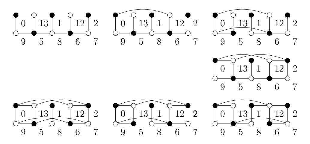
Figure 7. α-labeling of grid-like graphs.
Corollary 1. For positive integers t and n, C4t × Pn ∪ Pn is an α-graph.
Proof. We need to prove that C4t can be obtained from P4t+1 via a sequence of elementary transformations. Thus, suppose that v1, v2, . . . , v4t+1 are the consecutive vertices of P4t+1. The edge v2t+1v2t+2 is replaced with v2v4t+1. For every j ∈ {1, 2, . . . , t}, the edge v2jv2j+1 is replaced with v2j−1v2j+2. Note that in the first transformation x = 2t − 1 and in all the remaining ones, x = 1. Moreover, both extreme vertices of P4t+1 have now degree 2. In order to see that the resulting graph is actually C4t+1 ∪ P1 we must observe that now v1, v4, v3, v6, v5, v8, v7, . . . , v2t−1, v2t+2 are consecutive vertices. This implies that every vertex has degree 2 except v2t+1 that has degree 0. Since the edges v2t+2v2t+3, v2t+3v2t+4, . . . , v4tv4t+1 have not been touched, and v2t+2 is connected to v2t−1 as well as v2 is connected to v4t+1, we can see that our claim is true. Therefore, if these transformations are applied to every copy of P4t+1 within P4t+1 × Pn, the resulting graph is in fact C4t × Pn ∪ Pn.
In Figure 8 we show an example of this result for t = 3 and n = 4.
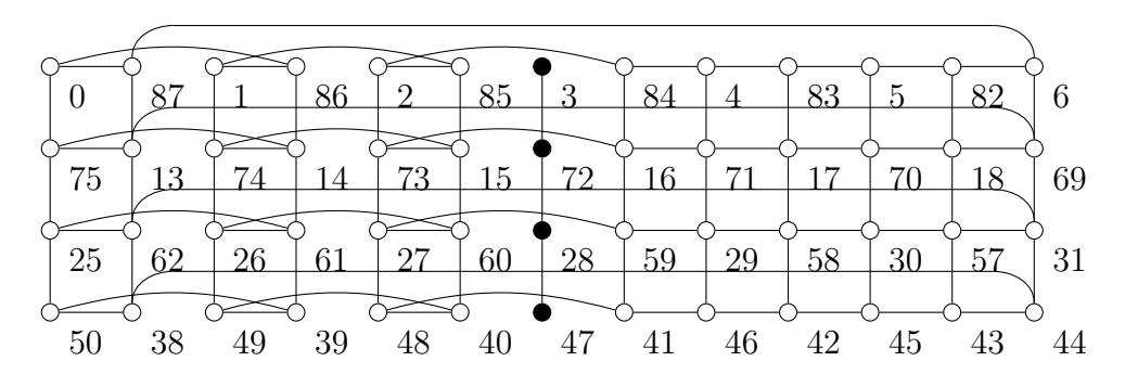
Figure 8. α-labeling of C13 × P4 ∪ P4
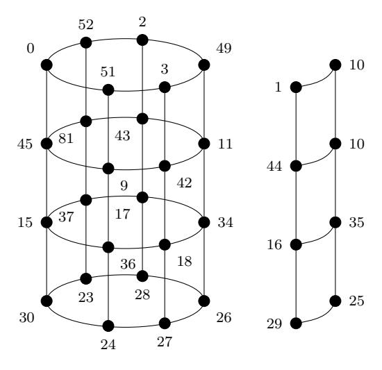
Figure 9. α-labeling of C6 × P4 ∪ P2 × P4
Corollary 2. For every t ≥ 2 and n ≥ 1, the graph C2t × Pn ∪ Pt−1 × Pn is an α-graph.
Proof. Let t ≥ 2 be an integer. Suppose that v1, v2, . . . , v3t−1 are the consecutive vertices of P3t−1 and that they have been labeled using Proposition 1, in such a way that v1 receives the label 0. If for every 2 ≤ i ≤ 3t − 3, the edge vivi+1 is replaced by the edge vi−1vi+2, then the paths hv1, v4, . . . , v3t−2i, hv2, v5, . . . , v3t−1i, and hv3, v6, . . . , v3t−3i are mutually disjoint.
Considering that the edges v2v3 and v3t−3v3t−2 have been replaced, the vertices v3 and v3t−3 have now degree one. In addition, the edges v1v2 and v3t−2v3t−1 have not been replaced, which implies that all the vertices, except v3 and v3t−3, have degree two and the graph induced by the vertices in {vi : i 6≡ 0(mod 3)} is a cycle of length 2t with consecutive vertices v1, v4, . . . , v3t−2, v3t−1, . . . , v5, v2, v1.
Since the α-labeling of P3t−1 has not been affected by these substitutions, the resulting graph, C2t∪Pt−1 is an α-graph. When the same substitutions are made on each copy of P3t−1 in P3t−1×Pn, we obtain an α-labeling of the graph C2t × Pn ∪ Pt−1 × Pn.
In Figure 9 we show an example of this construction for the case t = 3 and n = 4.
Acknowledgement
We want to thank the referee for his/her valuable comments and suggestions.
References
- [1] B.D. Acharya, Are all polyominoes arbitrarily graceful?, Proc. First Southeast Asian Graph Theory Colloquium, Ed. K.M. Koh and H.P. Yap, Springer-Verlag, N. Y. 1984, 205–211.
- [2] C. Balbuena, P. Garc´ıa-Vazquez, X. Marcote and J.C. Valenzuela, trees having an even or ´ quasi even degree sequence are graceful, Appl. Math. Lett. 20 (2007) 370-375.
- [3] C. Barrientos, Graceful graphs with pendant edges, Australas. J. Combin. 33 (2005), 99–107.
- [4] C. Barrientos and S. Minion, Alpha labelings of snake polyominoes and hexagonal chains, Bull. Inst. Combin. Appl. 74 (2015), 73–83.
- [5] C. Barrientos and S. Minion, Constructing graceful graphs with caterpillars, J. Algorithms and Computation 48 (2016), 117–125.
- [6] C. Barrientos and S. Minion, On the graceful Cartesian product of alpha-trees, Theory Appl. Graphs 4 (2017), No. 1, Art. 3, 12 pp.
- [7] C. Barrientos and S. Minion, Snakes: from graceful to harmonious Bull. Inst. Combin. Appl. 79 (2017), 95–107.
- [8] G. Chartrand and L. Lesniak, Graphs & Digraphs 2nd ed., Wadsworth & Brooks/Cole (1986).
- [9] J.A. Gallian, A dynamic survey of graph labelings, Electron. J. Combin. (2018), #DS6.
- [10] D. Jungreis and M. Reid, Labeling grids, Ars Combin., 34 (1992), 167–182.
- [11] D. Mishra, S.K. Rout and P.C. Nayak, Some new graceful generalized classes of diameter six trees, Electron. J. Graph Theory Appl. 5(1) (2017), 94–111.
- [12] S. Mitra and S. Bhoumik, Graceful labeling of triangular extension of complete bipartite graph, Electron. J. Graph Theory Appl. 7(1) (2019), 11–30.
- [13] A. Rosa, On certain valuations of the vertices of a graph, Theory of Graphs (Internat. Symposium, Rome, July 1966), Gordon and Breach, N. Y. and Dunod Paris (1967), 349–355.