Electronic Journal of Graph Theory and Applications

Wai Chee Shiu^a, Richard M. Low^b

^aDepartment of Mathematics, The Chinese University of Hong Kong, Shatin, N.T., Hong Kong, P.R. China ^bDepartment of Mathematics and Statistics, San Jose State University, San Jose, CA 95192, USA

shiu1958@gmail.com, richard.low@sjsu.edu

Let G=(V,E) be a simple connected graph. An injective function \(f:V\to\mathbb{R}^n\) is called an n-dimensional (or n-D) orthogonal labeling of G if \(uv,uw\in E\) implies that \((f(v)-f(u))\cdot (f(w)-f(u))=0\), where \(\cdot\) is the usual dot product in Euclidean space. If such an orthogonal labeling f of G exists, then G is said to be embedded in \(\mathbb{R}^n\) orthogonally. Let the orthogonal rank or(G) of G be the minimum value of G, where G admits an G-D orthogonal labeling (otherwise, we define G-G-G-G-G-G-G-G-G-G-

Keywords: orthogonal labeling, graph embedding, orthogonal drawing, Euclidean space 2010 Mathematics Subject Classification: 05C78, 05C10

DOI: 10.5614/ejgta.2019.7.2.13

1. Introduction

Graph labelings form an important part of graph theory. First formally introduced in the 1960s by Alex Rosa, this area of research has been the subject matter for many papers in the mathematical literature. Certain types of graph labelings have applications to graph decomposition problems, radar pulse code designs, X-ray crystallography and communication network models. The interested reader is directed to J.A. Gallian's comprehensive dynamic survey on graph labelings [2].

Received: 30 March 2018, Revised: 21 May 2019, Accepted: 1 June 2019.

For concepts and notation not explicitly defined in this paper, the reader is directed to [1]. In this paper, G = (V, E) is a simple connected graph. Let \(\Delta(G)\) denote the maximum degree of G. In [3], the following type of graph labeling was introduced:

• An injective function \(f: V \to \mathbb{R}^{\Delta(G)}\) is an orthogonal labeling of G if \(uv, uw \in E\) implies that \((f(v) - f(u)) \cdot (f(w) - f(u)) = 0\), where \(\cdot\) is the usual dot product in Euclidean space. If G has such a labeling, then G is called an orthogonal graph.

In their paper [3], Immanuel and Sugeng showed that the hypercubes \(Q_n\) \((n \ge 1)\), \(C_{2k}\) \((k \ge 2)\) and trees are orthogonal. They also showed that odd cycles, as well as any G containing \(K_3\) as a subgraph, are not orthogonal.

An orthogonal labeling of G can be explicitly constructed from a rectilinear drawing of G in \(\mathbb{R}^{\Delta(G)}\), where incident edges of G are perpendicular to each other. This particular type of labeling is quite interesting as it imposes a geometric structure to a graph. In fact, othogonal drawings of G (where \(\Delta(G)=2\)) have been studied extensively in computational geometry and computer science. As of this writing, a key phrase search for "orthogonal drawing" yields 111 entries in the MathSciNet database.

In this paper, we give further analysis of orthogonal graphs in a more general context. We start with a few definitions. For a graph G=(V,E), an injective function \(f:V\to\mathbb{R}^n\) is an n-dimensional (or n-D) orthogonal labeling of G if \(uv,uw\in E\) implies that \((f(v)-f(u))\cdot(f(w)-f(u))=0\), where \(\cdot\) is the usual dot product in Euclidean space. Let the orthogonal rank of G (denoted by or(G)) be the minimum value of n such that G admits an n-D orthogonal labeling (if any), otherwise define \(or(G)=\infty\). If \(or(G)=\Delta(G)\), then G is called an orthogonal graph.

Observations.

• 1. If G has an n-D orthogonal labeling, then \(n \geq \Delta(G)\).
• 2. Suppose H is a subgraph of a graph G. Then, \(or(H) \leq or(G)\).

2. Some results

For convenience, we will use v to denote the vertex label f(v) and uv to denote the vector f(v) - f(u), for \(u, v \in V(G)\), when there is no danger for confusion.

Lemma 2.1. \[or(K_{2,3}) = \infty\].

Proof. Let (X,Y) be the vertex set bipartition of \(K_{2,3}\), where \(X=\{x_1,x_2\}\) and \(Y=\{y_1,y_2,y_3\}\). Suppose there is an n-D orthogonal labeling f of \(K_{2,3}\), where \(3\leq n<\infty\). Without loss of generality, assume that \(x_1=(0,\ldots,0),\ y_1=(a_1,0,\ldots,0),\ y_2=(0,a_2,0,\ldots,0)\) and \(y_3=(0,0,a_3,0,\ldots,0),\) for some \(a_i\in\mathbb{R}\setminus\{0\},\ 1\leq i\leq 3.\) Now, suppose that \(x_2=(p_1,p_2,p_3,\ldots,p_n).\) Then, \(y_1x_2=(p_1-a_1,p_2,p_3,\ldots,p_n),\ y_2x_2=(p_1,p_2-a_2,p_3,\ldots,p_n)\) and \(y_3x_2=(p_1,p_2,p_3-a_3,\ldots,p_n).\) Since \(y_1x_1\) and \(y_1x_2\) are orthogonal, we have \(a_1(p_1-a_1)=0.\) Since \(a_1\neq 0\), this implies that \(a_1=a_2.\) Similarly, we have \(a_2=a_2.\) Since \(a_1=a_3.\) Since \(a_1=a_3.\) Since \(a_1=a_3.\) Since \(a_1=a_3.\) Since \(a_1=a_3.\) Since \(a_1=a_3.\) Since \(a_1=a_3.\) Since \(a_1=a_3.\) Since \(a_1=a_3.\) Since \(a_1=a_3.\) Since \(a_1=a_3.\) Since \(a_1=a_3.\) Since \(a_1=a_3.\) Since \(a_1=a_3.\) Since \(a_1=a_3.\) Since \(a_1=a_3.\) Since \(a_1=a_3.\) Since \(a_1=a_3.\) Since \(a_1=a_3.\) Since \(a_1=a_3.\) Since \(a_1=a_3.\) Since \(a_1=a_3.\) Since \(a_1=a_3.\) Since \(a_1=a_3.\) Since \(a_1=a_3.\) Since \(a_1=a_3.\) Since \(a_1=a_3.\) Since \(a_1=a_3.\) Since \(a_1=a_3.\) Since \(a_1=a_3.\) Since \(a_1=a_3.\) Since \(a_1=a_3.\) Since \(a_1=a_3.\) Since \(a_1=a_3.\) Since \(a_1=a_3.\) Since \(a_1=a_3.\) Since \(a_1=a_3.\) Since \(a_1=a_3.\) Since \(a_1=a_3.\) Since \(a_1=a_3.\) Since \(a_1=a_3.\) Since \(a_1=a_3.\) Since \(a_1=a_3.\) Since \(a_1=a_3.\) Since \(a_1=a_3.\) Since \(a_1=a_3.\) Since \(a_1=a_3.\) Since \(a_1=a_3.\) Since \(a_1=a_3.\) Since \(a_1=a_3.\) Since \(a_1=a_3.\) Since \(a_1=a_3.\) Since \(a_1=a_3.\) Since \(a_1=a_3.\) Since \(a_1=a_3.\) Since \(a_1=a_3.\) Since \(a_1=a_3.\) Since \(a_1=a_3.\) Since \(a_1=a_3.\) Since \(a_1=a_3.\) Since \(a_1=a_3.\) Since \(a_1=a_3.\) Since \(a_1=a_3.\) Since \(a_1=a_3.\) Since \(a_1=a_3.\) Since \(a_1=a_3.\) Since \(a_1=a_3.\) Since \(a_1=a_3.\) Since \(a_1=a_3.\) Since \(a_1=a_3.\) Since \(a_1=a_3.\) Since \(a_1=a_3.\) Since \(a_1=a_3.\) Since \(a_1=a_3.\) Since \(a_1=a_3.\) Since \(a_1=a_3.\) Since \(a_1=a_3.\) Since \(a_1=a_3.\) Since \(a_1=a_3.\) Since \(a_1=a_3.\) Since \(a_1=a_3.\) Since \(a_1=a_3.\) Since \(a_1=\)

Corollary 2.2. Suppose G contains \(K_{2,3}\). Then, \(or(G) = \infty\).

Proof. This follows immediately from Lemma 2.1 and Observation 2.

Corollary 2.3. \(or(K_{m,n}) = \infty\), for \(2 \le m \le n\), where m, n are not simultaneously equal to 2. Furthermore, \(or(K_{2,2}) = 2\).

Proof. In [3], it was shown that all even cycles are orthogonal. Thus, \(or(K_{2,2}) = 2\). The remainder of the claim follows immediately from Corollary 2.2.

Let \(G_i\), \(1 \le i \le n\), be n disjoint graphs. Suppose \(u_i \in V(G_i)\). Let H be the graph obtained from the \(G_i\) by identifying all the \(u_i\) to a single vertex. We say that H is a one-point union of the \(G_i\), where \(1 \le i \le n\).

Lemma 2.4. Let G' be a one-point union of arbitrary graphs G and H, with identified vertex w. Then, \(or(G') = \max\{or(G), or(H), \deg(w)\}.\)

Proof. If \(or(G) = \infty\) or \(or(H) = \infty\), then the result is obvious. So, we assume that or(G) = g and or(H) = h. Let w be the vertex in G' after merging \(u \in V(G)\) and \(v \in V(H)\). Clearly, \(or(G') \ge \max\{or(G), or(H), \deg(w)\}\).

We need to show that \(or(G') \leq \max\{or(G), or(H), \deg(w)\}\). Let \(\alpha: V(G) \to \mathbb{R}^g\) and \(\beta: V(H) \to \mathbb{R}^h\) be g-D and h-D orthogonal labelings of G and H, respectively. Without loss of generality, let \(1 \leq h \leq g\). Let the neighborhood of u in G be \(\{u_1, \ldots, u_m\}\) and the neighborhood of v in H be \(\{v_1, \ldots, v_n\}\). Clearly, \(m \leq g\) and \(n \leq h\).

Case 1: Suppose \(m+n \leq g\). By using rotation and translation, we can assume that \(\alpha(u)\) is the origin in \(\mathbb{R}^g\) and each edge \(\alpha(u)\alpha(u_i)\) lies on the positive i-th axis, \(1 \leq i \leq m\). Moreover, we can also assume that \(\alpha(V(G))\) lies in the region \(\Omega_+ = \{(x_1, \ldots, x_g) \mid x_i \geq 0\}\). Similarly, we can assume that each edge \(\beta(v)\beta(v_j)\) lies on the negative (m+j)-th axis, \(1 \leq j \leq n\). Moreover, we can also assume that \(\beta(V(H))\) lies in the region \(\Omega_- = \{(x_1, \ldots, x_g) \mid x_i \leq 0\}\). Combining these two labelings, we have the required labeling of G' and or(G') = g = or(G).

Case 2: Suppose m+n>g. Now, we want to orthogonally embed G' in \(\mathbb{R}^{m+n}\). By using rotation and translation, we can assume that \(\alpha(u)\) is the origin in \(\mathbb{R}^{m+n}\) and each edge \(\alpha(u)\alpha(u_i)\) lies on the positive i-th axis, \(1\leq i\leq m\). Moreover, we can also assume that \(\alpha(V(G))\) lies in the region \(\Omega_+=\{(x_1,\ldots,x_g,0,\ldots,0)\in\mathbb{R}^{m+n}\mid x_i\geq 0,1\leq i\leq g\}\). Similarly, we can assume that each edge \(\beta(v)\beta(v_j)\) lies on the negative (m+j)-th axis, \(1\leq j\leq n\). Moreover, we can also assume that \(\beta(V(H))\) lies in the region \(\Omega_-=\{(x_1,\ldots,x_g,\ldots,x_{m+n})\mid x_i\leq 0,1\leq i\leq m+n\}\). Combining these two labelings, we have the required labeling of G' and \(or(G')=m+n=\deg(w)\).

Figure 1 illustrates Lemma 2.4. In the first graph, \(G_1\) is a one-point union of \(C_5\) and \(K_{1,3}\), with the identified vertex being a leaf of \(K_{1,3}\). In the second graph, \(G_2\) is another one-point union of \(C_5\) and \(K_{1,3}\), where the identified vertex is the vertex of degree three in \(K_{1,3}\).

Corollary 2.5. The one-point union of orthogonal graphs is orthogonal.

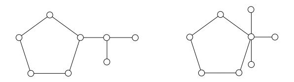
Figure 1. \(or(G_1) = 3\) and \(or(G_2) = 5\).

Proof. This follows immediately from Lemma 2.4.

Corollary 2.6. The one-point union of an orthogonal graph G and a tree T is orthogonal.

Proof. In [3], it was shown that every tree is orthogonal. Hence by Corollary 2.5, the claim is established. \(\Box\)

We note that Corollary 2.6 was also shown in [3].

Lemma 2.7. Let \(or(G), or(H) < \infty\) for graphs G and H, respectively. Then, \(\Delta(G) + \Delta(H) \le or(G \times H) \le or(G) + or(H)\).

Proof. Note that the maximum degree of \(G \times H\) is \(\Delta(G) + \Delta(H)\). So, the first inequality is obvious. Let \(f_G : V(G) \to \mathbb{R}^m\) and \(f_H : V(H) \to \mathbb{R}^n\), where \(or(G) \le m\) and \(or(H) \le n\). Define \(f : V(G) \times V(H) \to \mathbb{R}^{m+n}\) by \(f((u,v)) = (f_G(u), f_H(v))\), for \(u \in V(G)\) and \(v \in V(H)\). It is straightforward to check that f is an (m+n)-D orthogonal labeling of \(G \times H\), which establishes the second inequality.

Corollary 2.8. If G and H are orthogonal, then \(G \times H\) is orthogonal.

Proof. Let G and H be orthogonal graphs. Then, \(or(G) = \Delta(G)\) and \(or(H) = \Delta(H)\). Thus, by Lemma 2.7, the claim follows.

Lemma 2.9. Let K be a connected graph with cut-edge uv. Suppose K - uv = G + H (where \(u \in G\), \(v \in H\)) and or(G), \(or(H) < \infty\). Then, \(or(K) = \max\{or(G), or(H), \deg_K(u), \deg_K(v)\}\).

Proof. Clearly, \(or(K) \geq \max\{or(G), or(H), \deg_K(u), \deg_K(v)\}\). Let g = or(G) and h = or(H). Without loss of generality, assume \(1 \leq h \leq g\). Clearly, \(\deg_G(u) = m \leq g\) and \(\deg_H(v) = n \leq h\). Note that \(\deg_K(u) = m + 1 \leq g + 1\) and \(\deg_K(v) = n + 1 \leq h + 1 \leq g + 1\). Let \(\alpha: V(G) \to \mathbb{R}^g\) and \(\beta: V(H) \to \mathbb{R}^h\) be g-D and h-D orthogonal labelings, respectively. Let the neighborhood of u in G be \(\{u_1, \ldots, u_m\}\) and the neighborhood of v in H be \(\{v_1, \ldots, v_n\}\).

We first consider h < g.

<u>Case 1</u>: Suppose m < g. Then, \(\max\{or(G), or(H), \deg_K(u), \deg_K(v)\} = g\). It suffices to find a g-D orthogonal labeling for K. By using rotation and translation, we can assume that \(\alpha(u)\) is the origin in \(\mathbb{R}^g\) and each edge \(\alpha(u)\alpha(u_i)\) lies on the positive i-th axis, \(1 \le i \le m\). Moreover, we can also assume that \(\alpha(V(G))\) lies in the region \(\Omega_+ = \{(x_1, \ldots, x_g) \mid x_i \ge 0, 1 \le i \le g\}\). Similarly,

we can embed the graph H in \(\mathbb{R}^g\) such that \(\beta(v)\) is the origin of \(\mathbb{R}^g\) and each edge \(\beta(v)\beta(v_j)\) lies on the negative j-th axis, \(1 \leq j \leq n\). Moreover, we can also assume that \(\beta(V(H))\) lies in the region \(\Omega_- = \{(x_1, \ldots, x_g) \mid x_j \leq 0, 1 \leq j \leq g\}\). Finally, we translate \(\beta(V(H))\) one unit downward along the g-th axis. This gives us the required labeling.

<u>Case 2</u>: Suppose m = g. Then, \(\max\{or(G), or(H), \deg_K(u), \deg_K(v)\} = g + 1\). It suffices to find a (g + 1)-D orthogonal labeling for K. The proof is the same as in Case 1, by replacing g with g + 1.

Now, suppose h=g. Without loss of generality, we can assume that \(n \leq m\). The proof for this case is the same as above.

Thus, \[or(K) \leq \max\{or(G), or(H), \deg_K(u), \deg_K(v)\}\]. This completes the proof. \(\square\)

3. Applications

There is a 2-D orthogonal labeling of \(C_{2k}\) in [3]. Its restriction is a 2-D orthogonal labeling of \(P_{2k} = v_0v_1\cdots v_{2k-1}\) for \(k\geq 2\). For the sake of completeness, we list that labeling \(\phi\) here: \(\phi(v_0)=(0,0); \phi(v_{2r})=(r,k-r)\) for \(1\leq r\leq k-1;\) and \(\phi(v_{2r-1})=(r-1,k-r)\) for \(1\leq r\leq k.\) See Figure 2.

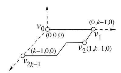
Figure 2. A 2-D orthogonal labeling of \(P_{2k}\) (drawn in \(\mathbb{R}^3\)).

For further use, we now introduce a 3-D orthogonal labeling of \(P_{2k+1} = v_0v_1u_0v_2\cdots v_{2k-1}\) such that the end vertices \(v_0\) and \(v_{2k-1}\) are embedded in x-axis, where \(k \geq 2\). Starting from the 2-D orthogonal labeling \(\phi\) for \(P_{2k} = v_0v_1\cdots v_{2k-1}\) shown above, we embed \(P_{2k}\) in the xy-path. Then, we embed the inserted vertex \(u_0\) at (1/2, k-1, 1/2). Clearly \(v_0v_1\bot v_1u_0\), \(v_1u_0\bot u_0v_2\) and \(u_0v_2\bot v_2v_3\).

Furthermore, we see that, \(v_{2k-1}v_0 \perp v_0 u_0\). Hence, we have the following theorem.

Theorem 3.1. For \[k \geq 2\], \(or(C_{2k}) = 2\) and \(or(C_{2k+1}) = 3\).

For an illustration of the above remarks and Theorem 3.1, see Figure 3.

Lemma 3.2. \(or(C_3) = \infty\).

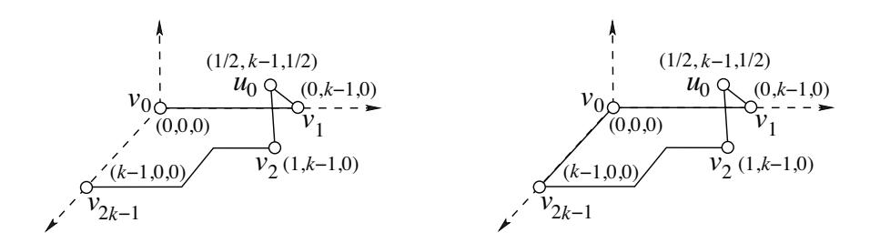
Figure 3. 3-D orthogonal labelings of \(P_{2k+1}\) and \(C_{2k+1}\), respectively.

Proof. Assume that \(or(C_3) = t\), for some finite t. Without loss of generality, let \(v_0\) be labeled with \((0,0,0,\ldots,0)\), \(v_1\) labeled with \((1,0,0,\ldots,0)\) and \(v_2\) labeled with \((0,c,0,\ldots,0)\). Then, \(v_2v_1 \perp v_0v_1\) implies \(1^2 + 0^2 + 0^2 + \cdots + 0^2 = 0\), which gives the desired contradiction.

We note that Lemma 3.2 is also mentioned in [3].

Corollary 3.3. If G is orthogonal, then \(G \times C_{2n}\) is orthogonal, for \(n \geq 2\).

Corollary 3.4. One-point union of n cycles is orthogonal, for \(n \geq 2\).

Proof. Let G be a one-point union of n cycles \(H_i\)'s. Note that \(or(H_i) = 2\) or 3, for each i. Consider n = 2 first. By Lemma 2.4, we have \(or(G) = \max\{or(H_1), or(H_2), 4\} = 4\). Now, we consider \(n \geq 3\). By applying Lemma 2.4 repeatedly, we see that the orthogonal rank of a one-point union of cycles is 2n, for \(n \geq 2\).

4. Bicyclic graphs without pendant

It is known that a bicyclic graph without pendant is a one-point union of two cycles, a theta graph or a long dumbbell graph [6]. In this section, we show that all bicyclic graphs without pendant are orthogonal.

Let U(m,n) be the one-point union of two cycles \(C_m = u_0u_1 \cdots u_{m-1}u_0\) and \(C_n = u_0u_mu_{m+1} \cdots u_{n+m-2}u_0\), where \(m, n \geq 3\). Corollary 3.4 shows that U(m,n) is orthogonal.

Definition 4.1. A theta graph is the union of three internally disjoint paths that have the same two distinct end vertices. Without loss of generality, we may assume that \(s \geq t \geq r \geq 1\) such that \(Q_s = u_0 u_1 \cdots u_s\), \(Q_t = u_0 u_{s+1} u_{s+2} \cdots u_{s+t-1} u_s\) and \(Q_r = u_0 u_{s+t} u_{s+t+1} \cdots u_{s+t+r-2} u_s\). Here, \(Q_i\) denotes a path of length i. We denote this graph by \(\Theta(s,t,r)\). Since we only consider simple graphs, at least two of \(s \geq t \geq 2\).

Definition 4.2. A long dumbbell graph is a graph obtained from two cycles \(C_m\) and \(C_n\), by joining a path \(Q_l\) of length l for \(m, n \geq 3\) and \(l \geq 1\). Without loss of generality, we can assume

\[C_m = u_0 u_1 \cdots u_{m-1} u_0, \quad Q_l = u_{m-1} u_m \cdots u_{m+l-1}\]

and \[C_n = u_{m+l-1}u_{m+l} \cdots u_{m+n+l-2}u_{m+l-1}\].

We denote this graph by D(m, n; l).

Theorem 4.1. The long dumbbell graph D(m, n; l) is orthogonal and or(D(m, n; l)) = 3, for \(m, n \geq 3\) and \(l \geq 1\).

Proof. Let uv be an edge in \(Q_l\). Let \(D(m,n;l) - uv = G_1 + G_2\). By Lemma 2.4, we have \(2 \le or(G_1) \le 3\) and \(2 \le or(G_2) \le 3\). Now \(\deg(u) = 1\) or 3 and \(\deg(v) = 1\) or 3. Applying Lemma 2.9, we have or(D(m,n;l)) = 3. Hence, D(m,n;l) is orthogonal.

Since \(\Theta(s,2,1)\) contains \(K_3\) and \(\Theta(2,2,2)\cong K_{2,3}\), their orthogonal ranks are infinity. Thus, we now only consider \(\Theta(s,t,1)\) when \(s\geq t\geq 3\), and \(\Theta(s,t,r)\) when \(s\geq t\geq 2\) but \((s,t,r)\neq (2,2,2)\).

Theorem 4.2. The theta graph \(\Theta(s,t,1)\) is orthogonal and \(or(\Theta(s,t,1))=3\), for \(s\geq t\geq 3\).

Proof. We keep the notation defined above. We embed \(Q_t\) (as well as \(Q_t \cup Q_1 \cong C_{t+1}\)) in the first octant such that \(u_0\) is the origin and \(u_s\) is the point \((\lceil t/2 \rceil - 1, 0, 0)\).

Individually, we may put \(Q_s\) in the fourth octant (i.e., the region \(\{(x,y,z) \mid x,z \geq 0, y \leq 0\}\)) such that \(u_0\) is the origin and \(u_s = (\lceil s/2 \rceil - 1, 0, 0)\). Scale down the image of \(Q_s\) by the rate \(\frac{\lceil t/2 \rceil - 1}{\lceil s/2 \rceil - 1}\) so that \(u_s\) becomes \((\lceil t/2 \rceil - 1, 0, 0)\). Hence, this labeling is the required orthogonal labeling. \(\square\)

Theorem 4.3. The theta graph \(\Theta(s,t,r)\) is orthogonal [except \(\Theta(2,2,2)\)] and \(or(\Theta(s,t,r))=3\), for s>t>r>2.

Proof. The labeling is similar to the proof of Theorem 4.2. We embed \(Q_t \cup Q_r \cong C_{t+r}\) in the first octant such that \(u_0\) is the origin and \(u_{s+1}\) is the point \((\lfloor (t+r)/2 \rfloor -1, 0, 0)\). Suppose the vertex \(u_s\) is put at the point \(\boldsymbol{w}\).

We view the ray from the origin to w as the positive x-axis on defining \(\phi\) or \(\psi\) above. By applying enlargement if necessary, we embed \(Q_s\) in the fifth octant (i.e., the region \(\{(x,y,z) \mid x,y \ge 0, z \le 0\}\)) such that \(u_0\) is the origin and \(u_s\) is w. Hence, this labeling is the required orthogonal labeling.

Hence, all bicyclic graphs without pendant (except \(\Theta(s,2,1)\) and \(\Theta(2,2,2)\)) are orthogonal.

5. Tessellation graphs

A tessellation is a tiling of the plane, using polygons. If a tessellation consists of congruent polygons, it is a regular tessellation. Thus, there are only three regular tessellations, utilizing equilateral triangles, squares, or regular hexagons. A tessellation graph is a finite subgraph of a regular tessellation, consisting of a grid of congruent polygons where each polygon shares at least one common edge with another.

Definition 5.1. A region \(\Omega\) in the plane is n-connected if the complement of \(\Omega\) has exactly n components.

Definition 5.2. For \(n \geq 2\), an n-tessellation graph is a graph which tessellates an n-connected region in the plane.

For example, a 1-tessellation graph tessellates a simply-connected, bounded region in the plane.

Consider a tessellation of the plane, using congruent equilateral triangles. Two triangles are connected if they share a common edge. Let T be a connected collection of triangles. Then, T is a connected planar graph, consisting of a grid of \(C_3\)'s with each \(C_3\) sharing at least one common edge with another. A connected collection of triangles is called a triomino. T is called an n-triomino if it is an n-tessellation graph.

Theorem 5.1. Let T be a 1-triomino. Then, \(or(T) = \infty\).

Proof. Every 1-triomino contains \(K_3\). Thus, the result follows immediately from \(or(K_3) = \infty\) and Observation 2.

A cell is the boundary of a unit square (\(\cong C_4\)) in the xy-plane, where the vertices of the square are at lattice points. Two cells are connected if they share a common edge. Let S be a connected collection of connected cells. Thus, S can be viewed as a connected planar graph, consisting of a grid of \(C_4\)'s with each \(C_4\) sharing at least one common edge with another. A connected collection of connected cells is called a polyomino.

Theorem 5.2. Every 1-polyomino is orthogonal.

Proof. Let P be a 1-polyomino. If \(P \cong P_n \times P_2\), then P is orthogonal by Corollary 2.8. Now, suppose that P is not isomorphic to \(P_n \times P_2\). Then, P is a subgraph of \(P_n \times P_m\), where \(m \geq 3\). Also, \(\Delta(P) = 4\). Thus, \(or(P) \geq 4\). Since \(or(P_n \times P_m) = 4\), we have that \(or(P) \leq 4\) by Observation 2. Hence, or(P) = 4.

Consider a tessellation of the plane, using congruent hexagons. Two hexagons are connected if they share a common edge. Let H be a connected collection of hexagons. Then, H is a connected planar graph, consisting of a grid of \(C_6\)'s with each \(C_6\) sharing at least one common edge with another. A connected collection of hexagons is called a honeycomb graph.

Here, we view such a graph (or benzenoid system) as a (finite) connected plane graph, where each inner face is a regular hexagon of side length one. The wall, which was defined in [4], is an infinite graph W=(V,E), where \(V=\mathbb{Z}\times\mathbb{Z}\) and \(\{(y_1,z_1),(y_2,z_2)\}\in E\) if: (1). \(z_1=z_2\) and \(|y_1-y_2|=1\); or (2). \(y_1=y_2,|z_1-z_2|=1\) and \(y_1+z_1+y_2+z_2\equiv 1\pmod 4\). See Figure 4.

<u>Remark.</u> Suppose (y, z) is a vertex of W. The neighborhood N(y, z) of (y, z) is as follows:

• For even y and even z, \(N(y, z) = \{(y 1, z), (y + 1, z), (y, z + 1)\}.\)
• For even y and odd z, \(N(y, z) = \{(y 1, z), (y + 1, z), (y, z 1)\}.\)
• For odd y and even z, \(N(y, z) = \{(y 1, z), (y + 1, z), (y, z 1)\}.\)
• For odd y and odd z, \(N(y, z) = \{(y 1, z), (y + 1, z), (y, z + 1)\}.\)

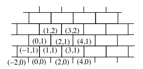
Figure 4. The wall W.

Note that a honeycomb graph is isomorphic to a subgraph of W.

Theorem 5.3. The wall W is orthogonal and or(W) = 3.

Proof. We embed the wall into the yz-plane first. That is, each vertex \((y_i, z_j)\) of the wall is located at \((0, y_i, z_j)\). Secondly, we move the point \((0, y_i, z_j)\) to \((1, y_i, z_j)\) when \(y_i\) is odd.

Now, for the point \((0,y_i,z_j)\) (i.e., \(y_i\) is even), its neighbors are \((1,y_i-1,z_j)\), \((1,y_i+1,z_j)\), \((0,y_i,z_j+\alpha)\), where \(\alpha\) is either 1 or -1. The vector raised from \((0,y_i,z_j)\) to these neighbors are (1,-1,0), (1,1,0) and \((0,0,\alpha)\). Clearly, they are mutually orthogonal. For the point \((1,y_i,z_j)\) (i.e., \(y_i\) is odd), its neighbors are \((0,y_i-1,z_j)\), \((0,y_i+1,z_j)\), \((1,y_i,z_j+\alpha)\). The vector raised from \((1,y_i,z_j)\) to these neighbors are (-1,-1,0), (-1,1,0) and \((0,0,\alpha)\). Clearly, they are also mutually orthogonal and or(W)=3.

Corollary 5.4. Every 1-tessellation honeycomb graph is orthogonal.

6. Acknowledgments

The authors are grateful to the anonymous referees. Their valuable comments and suggestions improved the final manuscript.

References

• [1] J.A. Bondy and U.S.R. Murty. Graph Theory with Applications, MacMillan, New York, (1976).
• [2] J.A. Gallian. A dynamic survey of graph labeling, Electron. J. Combin. 20 (2017), #DS6.
• [3] B. Immanuel and K.A. Sugeng. Orthogonal labeling, Indonesian Journal of Combinatorics. 1 (2016), 1-8.
• [4] W.C. Shiu and P.C.B. Lam. The Wiener number of the hexagonal net, Discrete Appl. Math. 73 (1997), 101-111.
• [5] W.C. Shiu and P.C.B. Lam. Wiener numbers of pericondensed benzenoid molecule systems, Congr. Numer. 126 (1997), 113-124.
• [6] W.C. Shiu and R.M. Low. The integer-magic spectra of bicyclic graphs without pendant, Congr. Numer. 214 (2012), 65-73.