Ravindra B. Bapat

Indian Statistical Institute, New Delhi, 110016, India

rbb@isid.ac.in

Let T be a tree with vertex set {1, . . . , n} such that each edge is assigned a nonzero weight. The squared distance matrix of T, denoted by ∆, is the n × n matrix with (i, j)-element d(i, j) 2 , where d(i, j) is the sum of the weights of the edges on the (ij)-path. We obtain a formula for the determinant of ∆. A formula for ∆⁻¹ is also obtained, under certain conditions. The results generalize known formulas for the unweighted case.

Keywords: tree, distance matrix, squared distance matrix, determinant, inverse

Mathematics Subject Classification: 05C50, 15A15

DOI: 10.5614/ejgta.2019.7.2.8

1. Introduction

Let G be a connected graph with vertex set V (G) = {1, . . . , n}. The distance between vertices i, j ∈ V (G), denoted d(i, j), is the minimum length (the number of edges) of a path from i to j (or an ij-path). We set d(i, i) = 0, i = 1, . . . , n. The distance matrix D(G), or simply D, is the n × n matrix with (i, j)-element dij = d(i, j).

A classical result of Graham and Pollak [7] asserts that if T is a tree with n vertices, then the determinant of the distance matrix D of T is (−1)ⁿ−¹ (n − 1)2ⁿ−² . Thus the determinant depends only on the number of vertices in the tree and not on the tree itself. A formula for the inverse of the distance matrix of a tree was given by Graham and Lovasz [6]. Several extensions and ´ generalizations of these results have been proved (see, for example [1], [2], [5], [8], [9] and the references contained therein).

Received: 12 October 2018, Accepted: 12 May 2019.

Let T be a tree with vertex set \(\{1, \ldots, n\}\) and let D be the distance matrix of T. The squared distance matrix \(\Delta\) is defined to be the Hadamard product \(D \circ D\), and thus has the (i, j)-element \(d(i, j)^2\). A formula for the determinant of \(\Delta\) was proved in [3], while the inverse and the inertia of \(\Delta\) were considered in [4].

In this paper we consider weighted trees. Let T be a tree with vertex set \(V(T) = \{1, \ldots, n\}\) and edge set \(E(T) = \{e_1, \ldots, e_{n-1}\}\). We assume that each edge is assigned a weight and let the weight assigned to \(e_i\) be denoted \(w_i\), which is a nonzero real number (not necessarily positive).

For \(i, j \in V(T), i \neq j\), the distance d(i, j) is defined to be the sum of the weights of the edges on the (unique) ij-path. We set d(i, i) = 0, i = 1, ..., n. Let D be the \(n \times n\) distance matrix with \(d_{ij} = d(i, j)\).

The Laplacian of T is the \(n \times n\) matrix defined as follows. The rows and the columns of L are indexed by V(T). For \(i \neq j\), the (i,j)-element is 0 if i and j are not adjacent. If i and j are adjacent, and if the edge joining them is \(e_k\), then the (i,j)-element of L is set equal to \(-1/w_k\). The diagonal elements of L are defined so that L has zero row (and column) sums.

The paper is organized as follows. In this section we review some basic properties of the distance matrix of a tree such as formulas for its determinant and inverse. Some preliminary results are obtained in Section 2. Sections 3 and 4 are devoted to the determinant and the inverse of \(\Delta\), respectively.

Example. Consider the tree

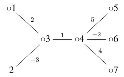
The Laplacian of the tree is given by

\[\begin{bmatrix} 1/2 & 0 & -1/2 & 0 & 0 & 0 & 0 \\ 0 & -1/3 & 1/3 & 0 & 0 & 0 & 0 \\ -1/2 & 1/3 & 7/6 & -1 & 0 & 0 & 0 \\ 0 & 0 & -1 & 19/20 & -1/5 & 1/2 & -1/4 \\ 0 & 0 & 0 & -1/5 & 1/5 & 0 & 0 \\ 0 & 0 & 0 & 1/2 & 0 & -1/2 & 0 \\ 0 & 0 & 0 & -1/4 & 0 & 0 & 1/4 \end{bmatrix}.\]

We let Q be the \(n \times (n-1)\) vertex-edge incidence matrix of the underlying unweighted tree, with an orientation assigned to each edge. Thus the rows and the columns of Q are indexed by V(T) and E(T) respectively. If \(i \in V(T), e_j \in E(T)\), the (i,j)-element of Q is 0 if i and \(e_j\) are not incident, it is 1(-1) if i and \(e_j\) are incident and i is the initial (terminal) vertex of \(e_j\). It is well-known [1] that Q has rank n-1 and any minor of Q is either 0 or \(\pm 1\) (thus Q is totally unimodular).

Let F be the n × n diagonal matrix with diagonal elements w1, . . . , wn−1. It can be verified that L = QF ⁻¹Q⁰ .

Lemma 1.1. The following assertions are true:

• (i) Q⁰DQ = −2F.
• (ii) LDL = −2L.

Proof. (i). The result follows from the following observation which is easily verified: If e^p = {i, j} and e^q = {k, `} are edges of T, then

\[d(i,k) + d(j,\ell) - d(i,\ell) - d(j,k)\]

equals 0 if e^p and e^q are distinct, and equals −2wp, if e^p = eq.

(ii). We have

\[LDL = QF^{-1}Q'DQF^{-1}Q'\] = \(QF^{-1}(-2F)F^{-1}Q'\) by (i) = \(-2QF^{-1}Q'\) = \(-2L\),

and the proof is complete.

Let δⁱ denote the degree of the vertex i, i = 1, . . . , n, and let δ be the n × 1 vector with components δ1, . . . , δn. We set τⁱ = 2 − δⁱ , i = 1, . . . , n, and let τ be the n × 1 vector with components τ1, . . . , τn.

Theorem 1.1. The following assertions are true:

• (i) det D = (−1)ⁿ−¹2 n−2 ( P ⁱ wi)(Q ⁱ wi).
• (ii) If P ⁱ wⁱ 6= 0, then D is nonsingular and

\[D^{-1} = -\frac{1}{2}L + \frac{1}{2\sum_{i} w_{i}} \tau \tau'.\]

(iii) Dτ = (P ⁱ wi)1.

Proof. Parts (i) and (ii) are well-known, see for example, [2]. To prove (iii), note that from (ii),

\[D^{-1}\mathbf{1} = \frac{1}{2\sum_{i} w_{i}} \tau \tau' \mathbf{1} = \frac{1}{\sum_{i} w_{i}} \tau,\]

since 1 0 τ = 2. It follows that Dτ = (P ⁱ wi)1 and the proof is complete.

2. Preliminary results

We now turn to the main results for the case of a weighted tree. Let T be a tree with vertex set \(V(T) = \{1, \ldots, n\}\) and edge set \(E(T) = \{e_1, \ldots, e_{n-1}\}\). Let \(w_1, \ldots, w_{n-1}\) be the edge-weights. Recall that \(\delta_i\) is the degree of vertex i and \(\tau_i = 2 - \delta_i\). We write \(j \sim i\) if vertex j is adjacent to vertex i. We let \(\hat{\delta}_i\) be the weighted degree of i, which is defined as

\[\hat{\delta}_i = \sum_{j:j\sim i} w(\{i,j\}), i = 1,\dots, n.\]

Let \(\hat{\delta}\) be the \(n \times 1\) vector with components \(\hat{\delta}_1, \dots, \hat{\delta}_n\).

Let \(\Delta\) be the squared distance matrix of T, which is the \(n \times n\) matrix with its (i, j)-element equal to \(d_{ij}^2\) or equivalently, \(d(i, j)^2\). The next result was obtained in [4] for the unweighted case,

Lemma 2.1. \(\Delta \tau = D\hat{\delta}\).

Proof. Let \(i \in \{1, ..., n\}\) be fixed. For \(j \neq i\), let \(\gamma(j)\) be the predecessor of j on the ij-path (in the underlying unoriented tree). Let \(e^j\) be the edge \(\{\gamma(j), j\}\) and set \(\theta^j = \hat{\delta}_j - w(e^j)\). We have

\[2\sum_{j=1}^{n} d(i,j)^{2}\] \[= \sum_{j=1}^{n} d(i,j)^{2} + \sum_{j\neq i} (d(i,\gamma(j)) + w(e^{j}))^{2}\] \[= \sum_{j=1}^{n} d(i,j)^{2} + \sum_{j\neq i} d(i,\gamma(j))^{2} + 2\sum_{j\neq i} d(i,\gamma(j))w(e^{j}) + \sum_{j\neq i} w(e^{j})^{2}.\] (1)

Note that

\[\sum_{j \neq i} d(i, \gamma(j))^2 = \sum_{j=1}^n (\delta_j - 1) d(i, j)^2, \tag{2}\]

since vertex j serves as a predecessor of \(\delta_j - 1\) vertices in paths from i. Also note that

\[\sum_{i \neq i} w(e^j)^2 = \sum_{k=1}^{n-1} w(e_k)^2.\] (3)

We have

\[\sum_{j=1}^{n} d(i,j)\hat{\delta}_{j}\] \[= \sum_{j\neq i} (d(i,\gamma(j) + w(e^{j}))(w(e^{j}) + \theta^{j})\] \[= \sum_{j\neq i} d(i,\gamma(j))w(e^{j}) + \sum_{j\neq i} w(e^{j})^{2} + \sum_{j\neq i} (d(i,\gamma(j)) + w(e^{j}))\theta^{j}.\] (4)

Observe that \(\theta^j\) is the sum of the weights of all the edges incident to j, except the edge \(e^j\), which is on the ij-path. Thus \((d(i,\gamma(j))+w(e^j))\theta^j\) equals \(\sum d(i,\gamma(\ell))w(e^\ell)\), where the summation is over all vertices adjacent to j, except i. Therefore it follows that

\[\sum_{j \neq i} d(i, \gamma(j)) w(e^j) = \sum_{j \neq i} (d(i, \gamma(j)) + w(e^j)) \theta^j.\] \[(5)\]

From (1)-(5) we get

\[2\sum_{i=1}^{n} d(i,j)^{2} = \sum_{j=1}^{n} d(i,j)^{2} \delta_{j} + \sum_{j=1}^{n} d(i,j) \hat{\delta}_{j},\]

which is equivalent to

\[\sum_{i=1}^{n} d(i,j)^{2} \tau_{j} = \sum_{j=1}^{n} d(i,j) \hat{\delta}_{j},\]

and the proof is complete.

Next we define the edge orientation matrix of T. We assign an orientation to each edge of T. Let \(e_i = (p,q)\); \(e_j = (r,s)\) be edges of T. We say that \(e_i\) and \(e_j\) are similarly oriented, denoted by \(e_i \Rightarrow e_j\), if d(p,r) = d(q,s). Otherwise \(e_i\) and \(e_j\) are said to be oppositely oriented, denoted by \(e_i \rightleftharpoons e_j\). For example, in the following diagram \(e_i\) and \(e_j\) are similarly oriented.

\[\circ p \longrightarrow \circ q - - - \circ r \longrightarrow \circ s\]

The edge orientation matrix of T is the \((n-1) \times (n-1)\) matrix H having the rows and the columns indexed by the edges of T. The (i,j)-element of H, denoted by h(i,j) is defined to be 1(-1) if the corresponding edges \(e_i, e_j\) of T are similarly (oppositely) oriented. The diagonal elements of H are set to be 1. We assume that the same orientation is used while defining the matrix H and the incidence matrix Q.

If the tree T has no vertex of degree 2, then we let \(\hat{\tau}\) be the diagonal matrix with diagonal elements \(1/\tau_1, \ldots, 1/\tau_n\). We state some basic properties of H next, see [3].

Theorem 2.1. Let T be a directed tree on n vertices, let H and Q be the edge orientation matrix and the vertex-edge incidence matrix of T, respectively. Then \(\det H = 2^{n-2} \prod_{i=1}^{n} \tau_i\). Furthermore, if T has no vertex of degree 2, then H is nonsingular and \(H^{-1} = \frac{1}{2}Q'\hat{\tau}Q\).

Let \(w_1, \ldots, w_{n-1}\) be the edge-weights. Recall that F be the diagonal matrix with diagonal elements \(w_1, \ldots, w_{n-1}\).

Also note that,

\[(FHF)_{ij} = \begin{cases} w_i w_j, & \text{if } e_i \Rightarrow e_j; \\ -w_i w_j, & \text{if } e_i \rightleftharpoons e_j. \end{cases}\]

Lemma 2.2. \(Q'\Delta Q = -2FHF\).

Proof. For \(i, j \in \{1, \dots, n-1\}\), let the edge \(e_i\) be from p to q and the edge \(e_j\) be from r to s. Then

\[(Q'\Delta Q)_{ij} = \begin{cases} d(p,r)^2 + d(q,s)^2 - d(p,s)^2 - d(q,r)^2, & \text{if } e_i \Rightarrow e_j; \\ d(p,s)^2 + d(q,r)^2 - d(p,r)^2 - d(q,s)^2, & \text{if } e_i \rightleftharpoons e_j. \end{cases}\](6)

Let \(d(r, s) = \alpha\). It follows from (6) that

\[(Q'\Delta Q)_{ij} = \begin{cases} (w_i + \alpha)^2 + (w_j + \alpha)^2 - (w_i + w_j + \alpha)^2 - \alpha^2 = -2w_i w_j, & \text{if } e_i \Rightarrow e_j; \\ (w_i + w_j + \alpha)^2 + \alpha^2 - (w_i + \alpha)^2 - (w_j + \alpha)^2 = 2w_i w_j, & \text{if } e_i \Rightarrow e_j; \\ = -2(FHF)_{ij}, \end{cases}\]

and the proof is complete.

Let \(\tilde{\tau}\) be the diagonal matrix with diagonal elements \(\tau_1, \ldots, \tau_n\).

Lemma 2.3. \(\Delta L = 2D\tilde{\tau} - 1\hat{\delta}'\).

Proof. Let \(i, j \in \{1, ..., n\}\) be fixed. Let vertex j have degree p. Suppose j is adjacent to vertices \(u_1, ..., u_p\) and let \(e_{\ell_1}, ..., e_{\ell_p}\) be the corresponding edges with weights \(w_{\ell_1}, ..., w_{\ell_p}\), respectively. We consider two cases.

Case 1. i = j. We have

\[(\Delta L)_{jj} = \sum_{k=1}^{n} d(j,k)^{2} \ell_{kj}\] \[= w_{\ell_{1}}^{2} (-w_{\ell_{1}})^{-1} + \dots + w_{\ell_{p}}^{2} (-w_{\ell_{p}})^{-1}\] \[= -(w_{\ell_{1}} + \dots + w_{\ell_{p}})\] \[= -\hat{\delta}_{j}.\]

Since the (j,j)-element of \(2D\tilde{\tau} - \mathbf{1}\hat{\delta}'\) is \(-\hat{\delta}_j\), the proof is complete in this case.

Case 2. \(i \neq j\). We assume, without loss of generality, that the ij-path passes through \(u_1\) (it is possible that \(i = u_1\)). Let \(d(i, j) = \alpha\). Then \(d(i, u_1) = \alpha - w_{\ell_1}, d(i, u_2) = \alpha + w_{\ell_2}, \dots, d(i, u_p) = \alpha\)

\(\alpha + w_{\ell_p}\). We have

\[(\Delta L)_{ij} = \sum_{k=1}^{n} d(i,k)^{2} \ell_{kj}\] \[= d(i,u_{1})^{2} (-w_{\ell_{1}})^{-1} + \cdots + d(i,u_{p})^{2} (-w_{\ell_{p}})^{-1} + d(i,j)^{2} \ell_{jj}\] \[= (\alpha - w_{\ell_{1}})^{2} (-w_{\ell_{1}})^{-1} + (\alpha + w_{\ell_{2}})^{2} (-w_{\ell_{2}})^{-1} + \cdots + (\alpha + w_{\ell_{p}})^{2} (-w_{\ell_{p}})^{-1}\] \[+ \alpha^{2} ((w_{\ell_{1}})^{-1} + \cdots + (w_{\ell_{p}})^{-1})\] \[= (-2\alpha w_{\ell_{1}} + w_{\ell_{1}}^{2})(-w_{\ell_{1}})^{-1} + (2\alpha w_{\ell_{2}} + w_{\ell_{2}}^{2})(-w_{\ell_{2}})^{-1} + \cdots\] \[+ (2\alpha w_{\ell_{p}} + w_{\ell_{p}}^{2})(-w_{\ell_{p}})^{-1}\] \[= 2\alpha - 2\alpha(p - 1) - (w_{\ell_{1}} + \cdots + w_{\ell_{p}})\] \[= 2\alpha \tau_{j} - (w_{\ell_{1}} + \cdots + w_{\ell_{p}}),\]

which is the (i, j)-element of \(2D\tilde{\tau} - \mathbf{1}\hat{\delta}'\) and the proof is complete.

3. Determinant

Our next objective is to obtain a formula for the determinant of the squared distance matrix. We first consider the case when the tree has no vertex of degree 2.

Theorem 3.1. Let T be a tree with vertex set \(V(T) = \{1, \ldots, n\}\), edge set \(E(T) = \{e_1, \ldots, e_{n-1}\}\), and edge weights \(w_1, \ldots, w_{n-1}\). Suppose T has no vertex of degree 2. Then

\[\det \Delta = (-1)^{n-1} \frac{4^{n-2}}{2} \prod_{i=1}^{n} \tau_i \prod_{i=1}^{n-1} w_i^2 \sum_{i=1}^{n} \frac{\hat{\delta}_i^2}{\tau_i}.\] (7)

Proof. We assign an orientation to the edges of the tree and let H and Q be, respectively, edge orientation matrix and the vertex-edge incidence matrix of T.

Let \(\Delta_i\) denote the i-th column of \(\Delta\), and let \(t_i\) be the column vector with 1 at the i-th place and zeros elsewhere, \(i = 1, \ldots, n\). Then

\[\begin{bmatrix} Q' \\ t'_1 \end{bmatrix} \Delta \begin{bmatrix} Q & t_1 \end{bmatrix} = \begin{bmatrix} Q'\Delta Q & Q'\Delta_1 \\ \Delta'_1 Q & 0 \end{bmatrix}. \tag{8}\]

Since \(\det \left[ \begin{array}{c} Q' \\ t_1' \end{array} \right] = \pm 1,\) it follows from (8) that

\[\det \Delta = \begin{bmatrix} Q' \Delta Q & Q' \Delta_1 \\ \Delta'_1 Q & 0 \end{bmatrix}\] \[= \begin{bmatrix} -2FHF & Q' \Delta_1 \\ \Delta'_1 Q & 0 \end{bmatrix} \text{ by Lemma 2.1}\] \[= (\det(-2FHF))(-\Delta'_1 Q(-2FHF)^{-1} Q' \Delta_1)\] \[= (-2)^{n-1} \prod_{i=1}^{n-1} w_i^2 (\det H) 2\Delta'_1 QF^{-1} H^{-1} F^{-1} Q' \Delta_1\] \[= (-1)^{n-1} 2^n \prod_{i=1}^{n-1} w_i^2 (\det H) \Delta'_1 QF^{-1} Q' \hat{\tau} QF^{-1} Q' \Delta_1, \tag{9}\]

in view of Theorem 2.1.

By Lemma 2.2 we have

\[\Delta_{1}'QF^{-1}Q'\hat{\tau}QF^{-1}Q'\Delta_{1} = \sum_{i} (2d_{1i}\tau_{i} - \hat{\delta}_{i})^{2} \frac{1}{\tau_{i}}\] \[= \sum_{i} (4d_{1i}^{2}\tau_{i}^{2} + \hat{\delta}_{i}^{2} - 4d_{1i}\tau_{i}\hat{\delta}_{i}) \frac{1}{\tau_{i}}\] \[= \sum_{i} 4d_{1i}^{2}\tau_{i} + \sum_{i} \frac{\hat{\delta}_{i}^{2}}{\tau_{i}} - 4\sum_{i} d_{1i}\hat{\delta}_{i}\] (10)

It follows from (10) and Lemma 2.1 that

\[\Delta_1' Q F^{-1} Q' \hat{\tau} Q F^{-1} Q' \Delta_1 = \sum_i \frac{\hat{\delta}_i^2}{\tau_i}.\] (11)

Also by Theorem 2.1,

\[\det H = 2^{n-2} \prod_{i=1}^{n} \tau_i. \tag{12}\]

The proof is complete by substituting (11) and (12) in (9).

Corollary 3.1. [3] Let T be an unweighted tree with vertex set \(V(T) = \{1, ..., n\}\). Suppose T has no vertex of degree 2. Then

\[\det \Delta = (-1)^n 4^{n-2} \left( 2n - 1 - 2 \sum_i \frac{1}{\tau_i} \right) \prod_{i=1}^n \tau_i.\] (13)

Proof. We set \(w_i = 1, i = 1, \dots, n-1\) in Theorem 3.1. Then \(\hat{\delta}_i = \delta_i = 2 - \tau_i, i = 1, \dots, n\). We have

\[\sum_{i} \frac{\delta_{i}^{2}}{\tau_{i}} = \sum_{i} \frac{(2 - \tau_{i})^{2}}{\tau_{i}}\] \[= \sum_{i} \frac{4 + \tau_{i}^{2} - 4\tau_{i}}{\tau_{i}}\] \[= 4 \sum_{i} \frac{1}{\tau_{i}} + \sum_{i} \tau_{i} - 4n\] \[= 4 \sum_{i} \frac{1}{\tau_{i}} + 2 - 4n\] \[= -2 \left(2n - 1 - 2 \sum_{i} \frac{1}{\tau_{i}}\right). \tag{14}\]

The proof is complete by substituting (14) in (7).

We turn to the case when there is a vertex of degree 2.

Theorem 3.2. Let T be a tree with vertex set \(V(T) = \{1, \ldots, n\}\), edge set \(E(T) = \{e_1, \ldots, e_{n-1}\}\), and edge weights \(w_1, \ldots, w_{n-1}\). Let q be a vertex of degree 2 and let p and r be neighbors of q. Let \(e_i = (pq), e_j = (qr)\). Then

\[\det \Delta = (-1)^{n-1} 2^{2n-5} (w_i + w_j)^2 \prod_{s=1}^{n-1} w_s^2 \prod_{k \neq a} \tau_k.\] (15)

Proof. We assume, without loss of generality, that \(e_i\) is directed from p to q and \(e_j\) is directed from q to r.

\[\circ p \xrightarrow{e_i} \circ q \xrightarrow{e_j} \circ r\]

Let \(z_q\) be the \(n \times 1\) unit vector with 1 at the q-th place and zeros elsewhere. Let \(\Delta_q\) be the q-th column of \(\Delta\). We have

\[\begin{bmatrix} Q' \\ z'_q \end{bmatrix} \Delta \begin{bmatrix} Q & z_q \end{bmatrix} = \begin{bmatrix} Q'\Delta Q & Q'\Delta_q \\ \Delta'_q Q & 0 \end{bmatrix} = \begin{bmatrix} -2FHF & Q'\Delta_q \\ \Delta'_q Q & 0 \end{bmatrix}, \tag{16}\]

in view of Lemma 2.2. It follows from (16) that

\[\begin{bmatrix} F^{-1} & 0 \\ 0 & 1 \end{bmatrix} \begin{bmatrix} Q' \\ z'_{a} \end{bmatrix} \Delta \begin{bmatrix} Q & z_{q} \end{bmatrix} \begin{bmatrix} F^{-1} & 0 \\ 0 & 1 \end{bmatrix} = \begin{bmatrix} -2H & F^{-1}Q'\Delta_{q} \\ \Delta'_{a}QF^{-1} & 0 \end{bmatrix}.\] (17)

Taking determinants of matrices in (17) we get

\[(\det F^{-1})^2 \det \Delta = \det \begin{bmatrix} -2H & F^{-1}Q'\Delta_q \\ \Delta'_q Q F^{-1} & 0 \end{bmatrix}.\] (18)

Note that the i-th and the j-th columns of H are identical.

Let H(j|j) denote the submatrix obtained by deleting row j and column j from H.

\(\ln \begin{bmatrix} -2H & F^{-1}Q'\Delta_q \\ \Delta_q'QF^{-1} & 0 \end{bmatrix}, \text{ subtract column } i \text{ from column } j, \text{ row } i \text{ from row } j, \text{ and then expand the determinant along column } j. \text{ Then we get}\)

\[\det \begin{bmatrix} -2H & F^{-1}Q'\Delta_q \\ \Delta'_q Q F^{-1} & 0 \end{bmatrix} = -((\Delta'_q Q F^{-1}))_j - (\Delta'_q Q F^{-1})_j)^2 \det(-2H(j|j))\]\[= -(-2)^{n-2} \det H(j|j)(-w_j - w_i)^2, \tag{19}\]

Note that H(j|j) is the edge orientation matrix of the tree obtained by deleting vertex q and replacing edges \(e_i\) and \(e_j\) by a single edge directed from p to r in the tree. Hence by Theorem 2.1,

\[\det H(j|j) = 2^{n-3} \prod_{k \neq q} \tau_k. \tag{20}\]

It follows from (17),(18) and (19) that

\[\det \Delta = -(\det F)^{2}(-1)^{n}2^{n-2}2^{n-3}(\prod_{k\neq q}\tau_{k})(w_{i} + w_{j})^{2}\] \[= (-1)^{n-1}2^{2n-5}(w_{i} + w_{j})^{2}\prod_{s=1}^{n-1}w_{s}^{2}\prod_{k\neq q}\tau_{k},\] (21)

and the proof is complete.

Corollary 3.2. Let T be a tree with vertex set \(V(T) = \{1, ..., n\}\), edge set \(E(T) = \{e_1, ..., e_{n-1}\}\), and edge weights \(w_1, ..., w_{n-1}\). Suppose T has at least two vertices of degree 2. Then \(\det \Delta = 0\).

Proof. The result follows from Theorem 3.2 since \(\tau_i = 0\) for at least two values of i.

4. Inverse

We now turn to the inverse of \(\Delta\), when it exists. When the tree has no vertex of degree 2, we can give a concise formula for the inverse. We first prove some preliminary results.

Lemma 4.1. Let the tree have no vertex of degree 2. Then

\[\Delta(2\tau - L\hat{\tau}\hat{\delta}) = (\hat{\delta}'\hat{\tau}\hat{\delta})\mathbf{1}.\] (22)

Proof. By Lemma 2.3, \(\Delta L = 2D\tilde{\tau} - 1\hat{\delta}'\). Hence

\[\Delta L \hat{\tau} \hat{\delta} = 2D \hat{\delta} - (\hat{\delta}' \hat{\tau} \hat{\delta}) \mathbf{1}. \tag{23}\]

Since by Lemma 2.1, \(\Delta \tau = D\hat{\delta}\), we obtain the result from (23).

For a square matrix A, we denote by cof A, the sum of the cofactors of A.

Lemma 4.2. Let T be a tree with vertex set \(V(T) = \{1, ..., n\}\), edge set \(E(T) = \{e_1, ..., e_{n-1}\}\), and edge weights \(w_1, ..., w_{n-1}\). Suppose T has no vertex of degree 2. Then

\[\cot \Delta = (-1)^{n-1} 2^{2n-3} \prod_{k=1}^{n-1} w_k^2 \prod_{i=1}^n \tau_i.\] (24)

Proof. By Lemma 2.2, \(Q'\Delta Q = -2FHF\). Taking determinant of both sides and using Cauchy-Binet formula, we get

\[cof \Delta = (-2)^{n-1} (\det F)^2 \det H = (-2)^{n-1} \prod_{k=1}^{n-1} w_k^2 2^{n-2} \prod_{i=1}^n \tau_i \text{ by Theorem 2.1} = (-1)^{n-1} 2^{2n-3} \prod_{k=1}^{n-1} w_k^2 \prod_{i=1}^n \tau_i,\] (25)

and the proof is complete.

Corollary 4.1. Let the tree have no vertex of degree 2 and let \(\beta = \hat{\delta}'\hat{\tau}\hat{\delta}\). If \(\beta \neq 0\), then \(\Delta\) is nonsingular and

\[\mathbf{1}'\Delta^{-1}\mathbf{1} = \frac{4}{\beta}.\tag{26}\]

Proof. Observe that \(\beta = \sum_{i=1}^{n} \frac{\hat{\delta}_{i}^{2}}{\tau_{i}}\). By Theorem 3.1,

\[\det \Delta = (-1)^{n-1} \frac{4^{n-2}}{2} \prod_{i=1}^{n} \tau_i \prod_{i=1}^{n-1} w_i^2 \sum_{i=1}^{n} \frac{\hat{\delta}_i^2}{\tau_i}.\] (27)

If \(\beta \neq 0\), then \(\Delta\) is nonsingular by (27). Note that \(\mathbf{1}'\Delta^{-1}\mathbf{1} = \frac{\cot \Delta}{\det \Delta}\). The proof is complete using Lemma 4.2 and (27).

Theorem 4.1. Let the tree have no vertex of degree 2 and let \(\beta = \hat{\delta}'\hat{\tau}\hat{\delta}\). Let \(\eta = 2\tau - L\hat{\tau}\hat{\delta}\). If \(\beta \neq 0\), then \(\Delta\) is nonsingular and

\[\Delta^{-1} = -\frac{1}{4}L\hat{\tau}L + \frac{1}{4\beta}\eta\eta'.\] (28)

Proof. Let \(X = -\frac{1}{4}L\hat{\tau}L + \frac{1}{4\beta}\eta\eta'\). Then

\[\Delta X = -\frac{1}{4}\Delta L\hat{\tau}L + \frac{1}{4\beta}\Delta\eta\eta'. \tag{29}\]

Squared distance matrix of a weighted tree Ravindra B. Bapat

By Lemma 2.3, \(\Delta L = 2D\tilde{\tau} - 1\hat{\delta}'\). Hence

\[\Delta L \hat{\tau} L = 2DL - \mathbf{1} \hat{\delta}' \hat{\tau} L. \tag{30}\]

Using Theorem 1.1, we can see that

\[DL = -2I + 1\tau'. \tag{31}\]

Finally, by Lemma 4.1, \(\Delta \eta = \beta\). This fact and (29), (30) and (31) lead to

\[\Delta X = I - \frac{1}{2} \mathbf{1} \tau' + \frac{1}{4} \hat{\delta}' \hat{\tau} L + \frac{1}{4\beta} \mathbf{1} \eta'. \tag{32}\]

Since \(\eta = 2\tau - L\hat{\tau}\hat{\delta}\), it follows from (32) that \(\Delta X = I\) and the proof is complete.

We conclude with an example to show that the condition \(\beta \neq 0\) is necessary in Theorem 4.1.

Example Consider the tree

\[\begin{array}{c|c} \circ 2 \\ \downarrow 1 \\ \circ 3 & 1 & 1 \\ \downarrow \gamma \\ \circ 4 \end{array}\]

The distance matrix of the tree is given by

\[D = \begin{bmatrix} 0 & 1 & 1 & \gamma & 1 \\ 1 & 0 & 2 & 1+\gamma & 2 \\ 1 & 2 & 0 & 1+\gamma & 2 \\ \gamma & 1+\gamma & 1+\gamma & 0 & 1+\gamma \\ 1 & 2 & 2 & 1+\gamma & 0 \end{bmatrix}.\]

It can be checked that \(\det \Delta = -32\gamma^2(\gamma^2-6\gamma-3)\). Thus \(\Delta\) is singular if \(\gamma=3+2\sqrt{3}\). Note that \(\hat{\delta}'=[\gamma+3,1,1,\gamma,1],\ \tau'=[-2,1,1,1,1]\) and hence, if \(\gamma=3+2\sqrt{3}\), then \(\sum_{i=1}^4\frac{\hat{\delta}^2}{\tau_i}=0\).

Acknowledgement

I sincerely thank Ranveer Singh for a careful reading of the manuscript. Support from the JC Bose Fellowship, Department of Science and Technology, Government of India, is gratefully acknowledged.

• [1] R.B. Bapat, Graphs and Matrices. Universitext. Springer, London; Hindustan Book Agency, New Delhi, 2010.
• [2] R.B. Bapat, S.J. Kirkland and M. Neumann, On distance matrices and Laplacians, Linear Algebra Appl. 401 (2005), 193–209.
• [3] R.B. Bapat and S. Sivasubramanian, Product distance matrix of a graph and squared distance matrix of a tree, Appl. Anal. Discrete Math. 7 (2013), no. 2, 285–301.
• [4] R.B. Bapat and S. Sivasubramanian, Squared distance matrix of a tree: inverse and inertia, Linear Algebra Appl. 491 (2016), 328–342.
• [5] R.B. Bapat, A.K. Lal and Sukanta Pati, A q-analogue of the distance matrix of a tree, Linear Algebra Appl. 416 (2006), 799–814.
• [6] R.L. Graham and L. Lovasz, Distance matrix polynomials of trees, ´ Adv. Math. 29 (1978), 60–88.
• [7] R.L. Graham and H.O. Pollak, On the addressing problem for loop switching, Bell System Tech. J. 50 (1971), 2495–2519.
• [8] Weigen Yan and Yeong-Nan Yeh, The determinants of q-distance matrices of trees and two quantities relating to permutations, Adv. in Appl. Math. 39 (2007), 311–321.
• [9] Hui Zhou and Qi Ding, The distance matrix of a tree with weights on its arcs, Linear Algebra Appl. 511 (2016), 365–377.