Electronic Journal of Graph Theory and Applications
Luis A. Dupont, Raquiel R. López Martínez, Miriam Rodríguez
Facultad de Matemáticas, Universidad Veracruzana, Circuito Gonzalo Aguirre Beltrán S/N; Zona Universitaria; Xalapa, Ver., México, CP 91090.
ldupont@uv.mx, ralopez@uv.mx, miriamrodriguezuv@gmail.com
The non-commuting graph \(\Gamma(G)\) of a non-abelian group G is defined as follows. The vertex set \(V(\Gamma(G))\) of \(\Gamma(G)\) is \(G \setminus Z(G)\) where Z(G) denotes the center of G and two vertices x and y are adjacent if and only if \(xy \neq yx\). We prove that the rainbow k-connectivity of \(\Gamma(G)\) is equal to \(\left\lceil \frac{k}{2} \right\rceil + 2\), for \(3 \leq k \leq |Z(G)|\).
Keywords: non-commuting graph, non-abelian group, rainbow connectivity, rainbow path
AMS Mathematics Subject Classification: 05C15, 05C25, 05C38
DOI: 10.5614/ejgta.2020.8.1.7
1. Introduction
Let G be a group and Z(G) be the center of G. The non-commuting graph \(\Gamma(G)\) associated to G is the graph with vertex set \(G \setminus Z(G)\) and such that two vertices x and y are adjacent whenever \(xy \neq yx\). The non-commuting graph of a group was first considered by Paul Erdös in 1975, [6]. Subsequently, it was strongly developed in [1].
Let \(\Gamma\) be a connected graph with the vertex set \(V(\Gamma)\) and the edge set \(E(\Gamma)\). Define a coloring \(\varphi: E(\Gamma) \to \{1, 2, \dots, t\}, t \in \mathbb{N}\), where adjacent edges may be colored the same. Given an edge coloring of \(\Gamma\), a path P is rainbow if no two edges of P are colored the same. An edge-colored
Received: 6 November 2018, Revised: 12 May 2019, Accepted: 27 June 2019.
graph \(\Gamma\) is rainbow connected if every pair of vertices of \(\Gamma\) are connected by a rainbow. The rainbow connection number \(\operatorname{rc}_1(\Gamma)\) of \(\Gamma\) is defined to be the minimum integer t such that there exists an edge-coloring of \(\Gamma\) with t colors that makes \(\Gamma\) rainbow connected.
From a generalization given by Chartrand, Johns, McKeon and Zhang in 2009 [2], an edge-colored graph \(\Gamma\) is called rainbow k-connected if any two distinct vertices of \(\Gamma\) are connected by at least k internally disjoint rainbow paths. The rainbow k-connectivity of \(\Gamma\), denoted by \(\operatorname{rc}_k(\Gamma)\), is the minimum number of colors required to color the edges of \(\Gamma\) to make it rainbow k-connected, and \(\varphi\) is called a rainbow k-coloring of \(\Gamma\). We usually denote \(\operatorname{rc}_1(\Gamma)\) by \(\operatorname{rc}(\Gamma)\).
The importance of rainbow connection number emerge from applications to the secure transfer of classified information between agencies [2]. Recently, Septyanto in [8], showed another form to see the application.
The commutator of an ordered pair \(g_1, g_2\) of elements of G is the element
\[[g_1, g_2] = g_1^{-1} g_2^{-1} g_1 g_2 \in G\]
G is abelian if and only if \([g_1, g_2] = 1\)
Let G(V, E), and let \(a = (e_1, ..., e_j)\) be a path with \(e_i \in E\). Then l(a) := j is called the length of a.
We denote by P(x,y) the set of all x,y paths in G. Then \(d(x,y) := min\{l(a)|a \in P(x,y)\}\) is called the distance from x to y.
We call \(diam(G) := max\{d(x,y)|x,y \in G\}\) the diameter of G. The length of a shortest cycle of G is called the girth of G.
When a pair of vertices \(g_i, g_j\) are joined, we denoted by \(g_i \sim g_j\). In otherwise we denoted by \(g_i \sim g_j\).
A non–commutative graph \(\Gamma(G)\) is connected and the diameter of \(\Gamma(G)\) is 2, \(diam(\Gamma(G))=2\).
Theorem 1.1. [1] For any non-abelian group G, \(diam(\Gamma(G)) = 2\). In particular, \(\Gamma(G)\) is connected.
In [9], it is shown that \(rc(\Gamma(G)) = rc_2(\Gamma(G)) = 2\).
Theorem 1.2. [9] Let G be a finite non-abelian group. Then \(rc(\Gamma(G)) = rc_2(\Gamma(G)) = 2\).
In the present article, we estimate \(rc_k(\Gamma(G))\) for \(3 \le k \le |Z(G)|\). Our main result is the following theorem.
Theorem 1.3. Let G be a finite non-abelian group. Then \(\operatorname{rc}_k(\Gamma(G)) \leq k\), for \(3 \leq k \leq |Z(G)|\) with \(|Z(G)| \geq 3\). Specifically \(\operatorname{rc}_k(\Gamma(G)) = \left\lceil \frac{k}{2} \right\rceil + 2\).
2. \(\operatorname{rc}_{\mathbf{k}}(\Gamma(G))\) with \(1 \leq k \leq |Z(G)|\)
Let G be a finite non-abelian group, from now on we write the vertices of \(\Gamma(G)\) as the partition
\[V(\Gamma(G)) = g_1 Z \dot{\cup} g_2 Z \dot{\cup} \cdots \dot{\cup} g_m Z,\]
with Z = Z(G), \(g_i Z \neq Z\), m = [G : Z(G)] - 1 and where \(g_i Z\) is an independent subset of \(\Gamma(G)\).
Proposition 2.1. Let G be a finite non-abelian group. Then the m-partite graph \(\Gamma(G)\) with partition \(V(\Gamma(G)) = g_1 Z \dot{\cup} g_2 Z \dot{\cup} \cdots \dot{\cup} g_m Z\), provides an adjacency by blocks.
Proof. Observe that every pair of vertices \(g_i \sim g_j\), if and only if for all \(x,y \in Z\) \(g_ix \sim g_jy\). In addition, for each i, the vertex \(g \in V(\Gamma(G))\) is adjacent to \(g_i\) if and only if it is adjacent to every element of the set \(g_iZ\). In other words, it is an adjacency by blocks.
Definition 2.2. Let G be a non-commutative finite group, with m-partition
\[V(\Gamma(G)) = g_1 Z \dot{\cup} g_2 Z \dot{\cup} \cdots \dot{\cup} g_m Z\]
adjacency by blocks. We define the skeleton of the m-partition as the subgraph induced by \(M = \{g_1, g_2, \dots, g_m\}\). The skeleton is denoted by \(S_{\Gamma(G)}^M\).
Remark 2.3. The graph \(\Gamma(G)\) is not complete , however \(S^M_{\Gamma(G)}\) can be complete, we can see this in the follow example: Let \(G = D_{2\times 4} := \langle a, x : a^4 = x^2 = 1, xax = a^{-1} \rangle\), the dihedral group of order 8. Then \(Z := Z(G) = \{1, a^2\}\), and we have
\[V(\Gamma(G)) = aZ\dot{\cup}xZ\dot{\cup}axZ.\]
Since each pair of \(\{a, x, ax\}\) do not commute, we have \(S^M_{\Gamma(D_{2\times 4})}\) is complete.
By Theorem 1.2, there is a coloration
\[\varphi: E(\Gamma(G)) \to \{1, 2\}\]
such that \(rc(\Gamma) = rc_2(\Gamma) = 2\). Thus, the graph \(\Gamma(G)\) is not complete, implies that \(\varphi(E(S^M_{\Gamma(G)})) = \{1, 2\}\). Therefore, the coloration
\[\phi := \varphi|_{E(S^M_{\Gamma(G)})} : E(S^M_{\Gamma(G)}) \to \{1, 2\}\]
meets the 2-connectivity, that is to say, \(rc(S^M_{\Gamma(G)}) \le 2\). Consider \(Z(G) = \{e = z_1, z_2, z_3, \dots, z_s\}\) and define the following coloring of \(\Gamma(G)\):
\[\psi: E(\Gamma(G)) \to \{1,2\} \text{ given by}\] \[\psi(\{g_iz_p,g_jz_p\}) = \phi(\{g_i,g_j\}) \text{ for } 1 \leq i,j,p \leq m; i \neq j;\] \[\psi(\{g_iz_p,g_jz_q\}) \neq \phi(\{g_i,g_j\}) \text{ for } 1 \leq i,j,p,q \leq m; i \neq j; p \neq q.\]
In the next section we give a coloring for \(3 \le k \le s\) with \(p \ne q\). Moreover in section 6 we will proof that this coloring works.
3. About edge-connectivity
We need to find k-rainbow paths between any two vertices for \(\Gamma(G)\), with \(k \geq 3\). We may ask for the maximum number of paths from \(v_1\) to \(v_2\) vertices, no two of which have an edge in common (such paths are called edge-disjoint paths). As a consequence of Menger's theorem about max-flow and min-cut, Witney [10] presented that a graph is k-connected if and only if any two vertices are connected by k internally disjoint paths. With Whitney's result we can answer how many edge-disjoint paths are connecting a given pair of vertices on \(\Gamma(G)\).
Definition 3.1. The edge-connectivity is the minimum size of a subset \(C \subset E(G)\) for which G - C is not connected for a graph G. The edge-connectivity of G is denoted by \(\lambda(G)\). If \(\lambda(G) \geq k\) then G es called k-edge connected.
The next theorem is a result implied by Menger's theorem. This form can be found in [7, Chapter 15].
Theorem 3.2. An undirected graph G = (V, E) is k-edge-connected if and only if there exist k edge-disjoint paths between any two vertices s and t.
As we can obtain the rainbow-connectivity number of \(\Gamma(G)\) and this graph is connected by blocks with s = |Z(G)| as size of each block, we have that the graph \(\Gamma(G)\) is s-edge-connected and there exist s edge-disjoint paths in \(\Gamma(G)\). Then, our problem now is coloring the s edge-disjoint paths of \(\Gamma(G)\).
Remark 3.3. By 1.1 we note that there exist two cases that we need analyze, for \(g_i, g_j, g_k, g_l \in S^M_{\Gamma(G)}\) and \(z_r, z_t, z_w, z_p \in Z(G)\). The first case is when \(g_i z_r \sim g_j z_t\) which give us a bipartite complete graph in \(\Gamma(G)\). The second case is when we have \(g_i z_r \sim g_j z_t \sim g_k z_w\), but \(g_i z_r \nsim g_k z_w\).
Remark 3.4. We note that \(\lambda(G) \geq s\). Then, if we want a path between end vertices \(g_i z_r\) and \(g_j z_t\), without loss of generality we start with \(g_i z_r\), necessarily, from 3.2, the edges \(g_i z_r \sim g_j z_{t_b}\) with \(t_b \in \{1, ..., s\}\), are in the set of edge-disjoint paths. The same happens for the edges \(g_i z_{r_a} \sim g_j z_t\) with \(r_a \in \{1, ..., s\}\) because we have s disjoint paths, therefore we need all outedge from \(g_i z_r\), and all in-edge to \(g_j z_t\), thus all our edge-disjoint paths have the following form: \((g_i z_r, g_j z_{t_b}, ..., g_i z_{r_a}, g_j z_t)\), with \(t_a, r_b \in \{1, ..., s\}\).
4. Rainbow k–connectivity
4.1. Case when \(g_i \sim g_j \in V(S^M_{\Gamma(G)})\)
Let s = |Z(G)| and let \(\bar{r} \equiv r \mod s\) with \(1 \leq r \leq s\). If \(g_i \sim g_j \in V(S^M_{\Gamma(G)})\), then the set of edges is given by
\[\text{[rumus tidak dapat ditampilkan dengan baik — lihat PDF asli]}\] \[E_2 = \begin{cases} \{e \in E(\Gamma(G)) | g_i z_r \sim g_j z_r \text{ such that } \psi(\{g_i z_p, g_j z_p\}) = 2\} \bigcup \\ \{e \in E(\Gamma(G)) | \text{ for } g_i z_r \sim g_j z_{\overline{r+1}} \text{ such that } \psi(\{g_i z_p, g_j z_p\}) = 1 \text{ with } \\ 1 \leq i, j, p \leq m; i \neq j \} \end{cases}\] \[E_3 = \{ \{e \in E(\Gamma(G)) | g_i z_r \sim g_j z_{\overline{r+2}} \} \}\] \[\vdots \qquad \vdots \qquad \vdots\] \[E_n = \{ \{e \in E(\Gamma(G)) | g_i z_r \sim g_j z_{\overline{r+n-1}} \} \}\] \[E_{n+1} = \{ \{e \in E(\Gamma(G)) | g_i z_r \sim g_j z_{\overline{r+n}} \} \}\] \[\text{[rumus tidak dapat ditampilkan dengan baik — lihat PDF asli]}\] with \(n = \lfloor \frac{k}{2} \rfloor\). The coloring given by: \[\text{[rumus tidak dapat ditampilkan dengan baik — lihat PDF asli]}\] \[f \mapsto i \text{ if } f \in E_i\]
For an easier study of this kind of graph we use a table called rainbow table, whose entries \((r_a, t_b)\) are the color from edge \((g_i z_{r_a}, g_j z_{t_b})\). This table is the following form:
\[\begin{array}{c} g_{j}z_{1} & g_{j}z_{2} & g_{j}z_{3} & \cdots & g_{j}z_{n} & g_{j}z_{n+1} & g_{j}z_{n+2} & \cdots & g_{j}z_{s} \\ g_{i}z_{1} & 1 & 2 & 3 & \cdots & n & n+1 \\ & & 1 & 2 & \cdots & n-1 & n & n+1 \\ & & & 1 & \cdots & n-2 & n-1 & n & \cdots \\ \vdots & \vdots & \vdots & \vdots & \vdots & \vdots \\ g_{i}z_{n} & & & 1 & 2 & 3 & \cdots & n+1 \\ \vdots & & & & & 1 & 2 & \cdots & n \\ \vdots & \vdots & & & & \vdots & \vdots \\ g_{i}z_{n} & & & & 1 & 2 & \cdots & n+1 \\ \vdots & & & & & \vdots & \vdots \\ g_{i}z_{s} & 2 & 3 & 4 & \cdots & n+1 & \vdots \\ & & & & & \vdots & \vdots \\ g_{i}z_{s} & & & & & 1 & 2 & \cdots & n \\ \end{array}\]
The (n+2)-color in the table is given by white space.
4.2. Case when \(g_i \sim g_j \sim g_l\) but \(g_i \nsim g_l\) in \(S_{\Gamma(G)}^M\)
Let s = |Z(G)| and let \(\bar{r} \equiv r \mod s\) with \(1 \leq r \leq s\). If \(g_i \sim g_j \in V(S^M_{\Gamma(G)})\), then the set of edges is given by
\[E_1 = \begin{cases} e \in E(\Gamma(G)) | g_i z_r \sim g_j z_r \text{ such that } \psi(\{g_i z_p, g_j z_p\}) = 1\} \bigcup \\ \{e \in E(\Gamma(G)) | \text{ for } g_i z_r \sim g_j z_{\overline{r+1}} \text{ such that } \psi(\{g_i z_p, g_j z_p\}) = 2 \text{ with } \\ 1 \leq i, j, p \leq m; i \neq j \end{cases}\] \[\text{[rumus tidak dapat ditampilkan dengan baik — lihat PDF asli]}\] \[E_3 = \{ e \in E(\Gamma(G)) | g_i z_r \sim g_j z_{\overline{r+2}} \}\] \[\vdots \quad \vdots \quad \vdots\] \[E_n = \{ e \in E(\Gamma(G)) | g_i z_r \sim g_j z_{\overline{r+n-1}} \}\] \[E_{n+1} = \{ e \in E(\Gamma(G)) | g_i z_r \sim g_j z_{\overline{r+n}} \}\] \[E_{n+2} = E(\Gamma(G)) \setminus (E_1 \cup \dots \cup E_{n+1})\] with \(n = \lceil \frac{k}{2} \rceil\). The coloring given by: \[\psi : E(\Gamma(G)) \longrightarrow \{1, \dots, n+2\}\] \[f \mapsto i \quad \text{ if } f \in E_i\]
This give us a table as:
\[\text{[rumus tidak dapat ditampilkan dengan baik — lihat PDF asli]}\]
Case when \(g_i \sim g_j \sim g_l\) but \(g_i \nsim g_l\) in \(S^M_{\Gamma(G)}\) with \(n = \left\lceil \frac{k}{2} \right\rceil\) and (n+2)-color with white spaces.
5. How to build the rainbow table
Example 5.1. We give the case when s=6 and \(g_1 \sim g_2\) in \(S_{\Gamma(G)}^M\) with the coloring assigned before. Without loss of generality suppose that \(\psi(\{g_1z_p,g_2z_p\})=1\), then the rainbow table is given by:
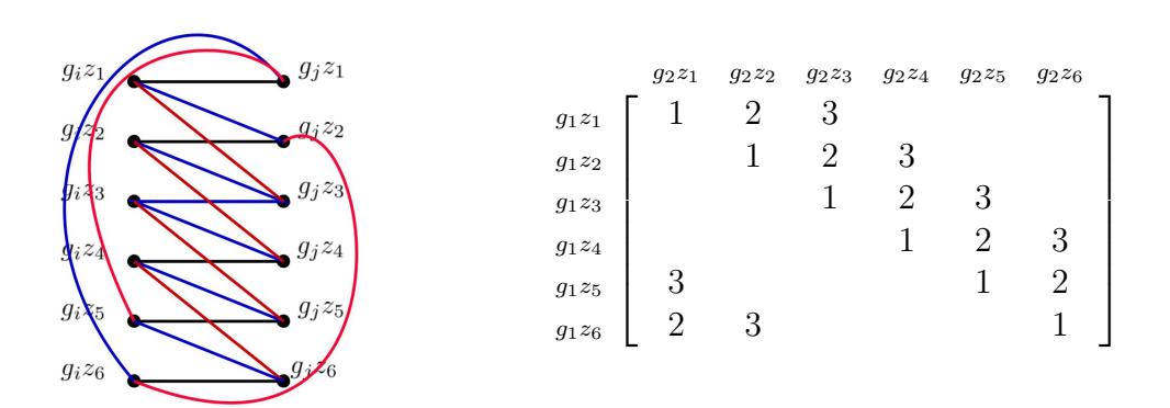
We can see that there is not exist a rainbow k-connectivity with 4 colors. To give s edge-disjoint paths with ends vertices \(g_1z_2\) and \(g_2z_4\), the first path cross above \(g_2z_1\), then we start the path with \(g_1z_2 \stackrel{4}{\sim} g_2z_1\). Now, we need move from \(g_2z_1\) but our only options are \(g_2z_1 \stackrel{1}{\sim} g_1z_1\), \(g_2z_1 \stackrel{3}{\sim} g_1z_5\) and \(g_2z_1 \stackrel{?}{\sim} g_1z_6\) and these edges can not arrive to \(g_2z_4\) because all the in-edge repeat color 4. For this reason we need to ensure that there exist enough in-edge that cover complete the out-edge in the set edges with majority color. For the existence of all edge-disjoint paths for any vertex we need to add one color more, and the table is given by
\[\text{[rumus tidak dapat ditampilkan dengan baik — lihat PDF asli]}\]
Example 5.2. We will do an example step-by-step about how we found all the edge-disjoint paths with our table. Let \(g_1 \sim g_2\) in \(S_{\Gamma(G)}^M\) and |Z(G)| = 4. Then, we will build our rainbow table with 3 colors the following form.
\[\text{[rumus tidak dapat ditampilkan dengan baik — lihat PDF asli]}\]
From this table we can found \(rc_3(\Gamma(G)) = 3\) for any vertices. For example, for end vertices \(g_1z_3, g_2z_4\)
\[\text{[rumus tidak dapat ditampilkan dengan baik — lihat PDF asli]}\]
If we note, we can not find 4 edge-disjoint paths with 3 colors, because \(g_1z_1\) to \(g_2z_1\) passes through \(g_2z_3\), the paths are the followings: \(g_1z_1 \stackrel{3}{\sim} g_2z_3 \stackrel{2}{\sim} g_1z_2 \stackrel{3}{\sim} g_2z_1\) or \(\text{[rumus tidak dapat ditampilkan dengan baik — lihat PDF asli]}\)\(g_2z_1\). Then, we need add another color, then the table is 4 colors the following form:
\[\text{[rumus tidak dapat ditampilkan dengan baik — lihat PDF asli]}\]
Then, with all this 4 colors we found all 4 edge-disjoint paths from \(g_1z_1\) to \(g_2z_1\), and they are the followings:
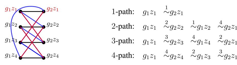
and the same is true for any pair of vertices.
6. Proofs
6.1. Case 3-partite with |Z(G)| = 3
The coloring given before can not help us to find all the disjoint-edge paths for the case when \(g_i \sim g_j \sim g_l\) but \(g_i \nsim g_l\) in \(S^M_{\Gamma(G)}\), for example, the rainbow table for this case is the next
\[\text{[rumus tidak dapat ditampilkan dengan baik — lihat PDF asli]}\]
But, we can see that for go from \(g_i z_1\) to \(g_l z_2\) we have same colors then, we need to do paths with length at least 4 like the following picture:

The coloring given for this specifical case is the following: The rainbow tables for each case
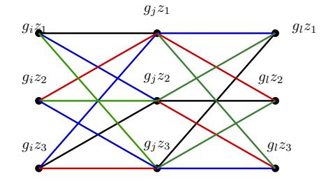
are the following:
\[\text{[rumus tidak dapat ditampilkan dengan baik — lihat PDF asli]}\]
Theorem 6.1. Let G be a non-abelian group with |Z(G)| = 3 and \(\Gamma(G)\) be the non-commutative graph associated to G, then \(rc_3(\Gamma(G)) = 4\).
Proof. Let the set of edges be the following form:
\[E_1 = \{e \in E(\Gamma(G)) | g_i z_{k_r} \sim g_j z_1 \text{ such that } \psi(\{g_i,g_j\}) = 1 \text{ for } g_i, g_j \in S^M_{\Gamma(G)} \text{ and } k_r = 1,2,3\}\] \[\bigcup \{e \in E(\Gamma(G)) | g_j z_2 \sim g_l z_2, g_j z_3 \sim g_l z_1 \text{ such that } \psi(\{g_j,g_l\}) = 2 \text{ for } g_j, g_l \in S^M_{\Gamma(S)}\}\] \[E_2 = \{e \in E(\Gamma(G)) | g_i z_{k_r} \sim g_j z_2 \text{ such that } \psi(\{g_i,g_j\}) = 1 \text{ for } g_i, g_j \in S^M_{\Gamma(G)} \text{ and } k_r = 1,2,3\}\] \[\bigcup \{e \in E(\Gamma(G)) | g_j z_{j_a} \sim g_l z_{j_a} \text{ such that } \psi(\{g_j,g_l\}) = 2 \text{ for } g_j, g_l \in S^M_{\Gamma(S)} \text{ and } j_a = 1,3\}\] \[E_3 = \{e \in E(\Gamma(G)) | g_i z_{k_r} \sim g_j z_3 \text{ such that } \psi(\{g_i,g_j\}) = 1 \text{ for } g_i, g_j \in S^M_{\Gamma(G)} \text{ and } k_r = 1,2,3\}\] \[\bigcup \{e \in E(\Gamma(G)) | g_j z_1 \sim g_l z_2, g_j z_2 \sim g_l z_3 \text{ such that } \psi(\{g_j,g_l\}) = 2 \text{ for } g_j, g_l \in S^M_{\Gamma(S)}\}\] \[E_4 = E \setminus (E_1 \cup E_2 \cup E_3)\]
And the coloring is given by
\[\psi: E(\Gamma(G)) \longrightarrow \{1, 2, 3, 4\}\] \[f \mapsto i \text{ if } i \in E_i.\]
The following are all the 3 edge-disjoint paths for each pair of vertices when \(\phi(\{g_j, g_l\}) = 2\)
| \(g_j z_1 \stackrel{2}{\sim} g_l z_1\) | \[g_j z_1 \stackrel{3}{\sim} g_l z_2\] | \(g_j z_1 \stackrel{4}{\sim} g_l z_3\) |
|---|---|---|
| \[g_j z_1 \stackrel{4}{\sim} g_l z_3 \stackrel{2}{\sim} g_j z_3 \stackrel{1}{\sim} g_l z_1\] | \[g_j z_1 \stackrel{2}{\sim} g_l z_1 \stackrel{1}{\sim} g_j z_3 \stackrel{4}{\sim} g_l z_2\] | \[g_j z_1 \stackrel{2}{\sim} g_l z_1 \stackrel{4}{\sim} g_j z_2 \stackrel{3}{\sim} g_l z_3\] |
| \[g_j z_1 \stackrel{3}{\sim} g_l z_2 \stackrel{1}{\sim} g_j z_2 \stackrel{4}{\sim} g_l z_1\] | \[g_j z_1 \stackrel{4}{\sim} g_l z_3 \stackrel{3}{\sim} g_j z_2 \stackrel{1}{\sim} g_l z_2\] | \[g_j z_1 \stackrel{3}{\sim} g_l z_2 \stackrel{4}{\sim} g_j z_3 \stackrel{2}{\sim} g_l z_3\] |
| \(g_j z_2 \stackrel{4}{\sim} g_l z_1\) | \[g_j z_2 \stackrel{1}{\sim} g_l z_2\] | \(g_j z_2 \stackrel{3}{\sim} g_l z_3\) |
| \[g_j z_2 \stackrel{1}{\sim} g_l z_2 \stackrel{3}{\sim} g_j z_1 \stackrel{2}{\sim} g_l z_1\] | \[g_j z_2 \stackrel{4}{\sim} g_l z_1 \stackrel{2}{\sim} g_j z_1 \stackrel{3}{\sim} g_l z_2\] | \[g_j z_2 \stackrel{4}{\sim} g_l z_1 \stackrel{1}{\sim} g_j z_3 \stackrel{2}{\sim} g_l z_3\] |
| \[g_j z_2 \stackrel{3}{\sim} g_l z_3 \stackrel{2}{\sim} g_j z_3 \stackrel{1}{\sim} g_l z_1\] | \[g_j z_2 \stackrel{3}{\sim} g_l z_3 \stackrel{2}{\sim} g_j z_3 \stackrel{4}{\sim} g_l z_2\] | \[g_j z_2 \stackrel{1}{\sim} g_l z_2 \stackrel{3}{\sim} g_j z_1 \stackrel{4}{\sim} g_l z_3\] |
| \(g_j z_3 \stackrel{1}{\sim} g_l z_1\) | \(g_j z_3 \stackrel{4}{\sim} g_l z_2\) | \(g_j z_3 \stackrel{2}{\sim} g_l z_3\) |
| \[g_j z_3 \stackrel{4}{\sim} g_l z_2 \stackrel{3}{\sim} g_j z_1 \stackrel{2}{\sim} g_l z_1\] | \[g_j z_3 \stackrel{1}{\sim} g_l z_1 \stackrel{2}{\sim} g_j z_1 \stackrel{3}{\sim} g_l z_2\] | \[g_j z_3 \stackrel{4}{\sim} g_l z_2 \stackrel{1}{\sim} g_j z_2 \stackrel{3}{\sim} g_l z_3\] |
| \[g_j z_3 \stackrel{2}{\sim} g_l z_3 \stackrel{3}{\sim} g_j z_2 \stackrel{4}{\sim} g_l z_1\] | \[g_j z_3 \stackrel{2}{\sim} g_l z_3 \stackrel{3}{\sim} g_j z_2 \stackrel{1}{\sim} g_l z_2\] | \[g_j z_3 \stackrel{1}{\sim} g_l z_1 \stackrel{2}{\sim} g_j z_1 \stackrel{4}{\sim} g_l z_3\] |
All the edge-disjoint paths when \(\phi(\{g_i,g_j\})=2, \phi(\{g_j,g_l\})=2\) and \(g_i\sim g_j\sim g_l\) but \(g_i\nsim g_l\)
| \(g_i z_1 \sim g_l z_1\) | \(g_i z_1 \sim g_l z_2\) | \(g_i z_1 \sim g_l z_3\) |
|---|---|---|
| \[g_{i}z_{1} \stackrel{1}{\sim} g_{j}z_{1} \stackrel{2}{\sim} g_{l}z_{1}\] \[g_{i}z_{1} \stackrel{2}{\sim} g_{j}z_{2} \stackrel{4}{\sim} g_{l}z_{1}\] \[g_{i}z_{1} \stackrel{4}{\sim} g_{j}z_{3} \stackrel{1}{\sim} g_{l}z_{2}\] | \[g_{i}z_{1} \stackrel{4}{\sim} g_{j}z_{3} \stackrel{2}{\sim} g_{l}z_{3} \stackrel{3}{\sim} g_{i}z_{2} \stackrel{1}{\sim} g_{l}z_{2}\] \[g_{i}z_{1} \stackrel{2}{\sim} g_{j}z_{2} \stackrel{1}{\sim} g_{i}z_{3} \stackrel{3}{\sim} g_{j}z_{3} \stackrel{4}{\sim} g_{l}z_{2}\] \[g_{i}z_{1} \stackrel{1}{\sim} g_{j}z_{1} \stackrel{3}{\sim} g_{l}z_{2}\] | 2 3 |
| \(g_i z_2 \sim g_l z_1\) | \(g_i z_2 \sim g_l z_2\) | \(g_i z_2 \sim g_l z_3\) |
|---|---|---|
| \[g_{i}z_{2} \stackrel{3}{\sim} g_{j}z_{1} \stackrel{2}{\sim} g_{j}z_{1}\] \[g_{i}z_{2} \stackrel{2}{\sim} g_{j}z_{3} \stackrel{3}{\sim} g_{i}z_{3} \stackrel{1}{\sim} g_{j}z_{2} \stackrel{4}{\sim} g_{l}z_{1}\] | \[\text{[rumus tidak dapat ditampilkan dengan baik — lihat PDF asli]}\] | |
| \(g_i z_2 \overset{4}{\sim} g_j z_2 \overset{3}{\sim} g_l z_3 \overset{2}{\sim} g_j z_3 \overset{1}{\sim} g_l z_1\) | \[\begin{vmatrix} g_i z_2 \stackrel{3}{\sim} g_j z_1 \stackrel{2}{\sim} g_l z_1 \stackrel{4}{\sim} g_j z_2 \stackrel{1}{\sim} g_l z_2 \end{vmatrix}\] | \[\begin{vmatrix} g_i z_2 \stackrel{?}{\sim} g_j z_3 \stackrel{4}{\sim} g_l z_2 \stackrel{1}{\sim} g_j z_2 \stackrel{3}{\sim} g_l z_3 \end{vmatrix}\] |
| \(g_i z_3 \sim g_l z_1\) | \[g_i z_3 \sim g_l z_2\] | \(g_i z_3 \sim g_l z_3\) |
|---|---|---|
| \[g_{i}z_{3} \stackrel{3}{\sim} g_{j}z_{3} \stackrel{1}{\sim} g_{l}z_{1}\] \[g_{i}z_{3} \stackrel{2}{\sim} g_{j}z_{1} \stackrel{3}{\sim} g_{l}z_{2} \stackrel{1}{\sim} g_{j}z_{2} \stackrel{4}{\sim} g_{l}z_{1}\] | \[\text{[rumus tidak dapat ditampilkan dengan baik — lihat PDF asli]}\] | \[g_i z_3 \stackrel{2}{\sim} g_j z_1 \stackrel{4}{\sim} g_l z_3\]\[g_i z_3 \stackrel{1}{\sim} g_j z_2 \stackrel{3}{\sim} g_l z_3\] |
| \[|g_i z_3 \stackrel{\cdot}{\sim} g_j z_2 \stackrel{\tau}{\sim} g_i z_2 \stackrel{\circ}{\sim} g_j z_1 \stackrel{\circ}{\sim} g_l z_1\] | \[\mid g_i z_3 \stackrel{\circ}{\sim} g_j z_3 \stackrel{\circ}{\sim} g_i z_2 \stackrel{\circ}{\sim} g_j z_2 \stackrel{\circ}{\sim} g_l z_2\] | \(g_i z_3 \stackrel{\circ}{\sim} g_j z_3 \stackrel{\circ}{\sim} g_l z_3\) |
All the edge-disjoint paths when \(\psi(\{g_i,g_j\})=1\)
| \(g_i z_1 \stackrel{1}{\sim} g_j z_1\) | \(\mid g_i z_1 \stackrel{2}{\sim} g_j z_2\) | \(g_i z_1 \stackrel{4}{\sim} g_j z_3\) |
| \[g_i z_1 \stackrel{2}{\sim} g_j z_2 \stackrel{4}{\sim} g_i z_2 \stackrel{3}{\sim} g_j z_1\] | \[g_i z_1 \stackrel{4}{\sim} g_j z_3 \stackrel{3}{\sim} g_i z_3 \stackrel{1}{\sim} g_j z_2\] | \[g_i z_1 \stackrel{2}{\sim} g_j z_2 \stackrel{1}{\sim} g_i z_3 \stackrel{3}{\sim} g_j z_3\] |
| \[g_i z_1 \stackrel{4}{\sim} g_j z_3 \stackrel{3}{\sim} g_i z_3 \stackrel{2}{\sim} g_j z_1\] | \[g_i z_1 \stackrel{1}{\sim} g_j z_1 \stackrel{3}{\sim} g_i z_2 \stackrel{4}{\sim} g_j z_2\] | \[g_i z_1 \stackrel{1}{\sim} g_j z_1 \stackrel{3}{\sim} g_i z_2 \stackrel{2}{\sim} g_j z_3\] |
| \(g_i z_2 \stackrel{3}{\sim} g_j z_2\) | \(g_i z_2 \stackrel{4}{\sim} g_j z_2\) | \(g_i z_2 \stackrel{2}{\sim} g_j z_3\) |
| \[g_i z_2 \stackrel{4}{\sim} g_j z_2 \stackrel{1}{\sim} g_i z_3 \stackrel{2}{\sim} g_j z_1\] | \[g_i z_2 \stackrel{3}{\sim} g_j z_1 \stackrel{1}{\sim} g_i z_1 \stackrel{2}{\sim} g_j z_2\] | \(g_i z_2 \stackrel{3}{\sim} g_j z_1 \stackrel{1}{\sim} g_i z_1 \stackrel{4}{\sim} g_j z_3\) |
| \[g_i z_2 \stackrel{2}{\sim} g_j z_3 \stackrel{4}{\sim} g_i z_1 \stackrel{1}{\sim} g_j z_1\] | \[g_i z_2 \stackrel{2}{\sim} g_j z_1 \stackrel{3}{\sim} g_i z_3 \stackrel{1}{\sim} g_j z_2\] | \[g_i z_2 \stackrel{4}{\sim} g_j z_2 \stackrel{1}{\sim} g_i z_3 \stackrel{3}{\sim} g_j z_3\] |
| \(g_i z_3 \stackrel{2}{\sim} g_j z_1\) | \(g_i z_3 \stackrel{1}{\sim} g_j z_2\) | \(g_i z_3 \stackrel{3}{\sim} g_j z_3\) |
| \[g_i z_3 \stackrel{1}{\sim} g_j z_2 \stackrel{4}{\sim} g_i z_2 \stackrel{3}{\sim} g_j z_1\] | \[g_i z_3 \stackrel{3}{\sim} g_j z_3 \stackrel{4}{\sim} g_i z_1 \stackrel{2}{\sim} g_j z_2\] | \[g_i z_3 \stackrel{1}{\sim} g_j z_2 \stackrel{4}{\sim} g_i z_2 \stackrel{2}{\sim} g_j z_3\] |
| \[g_i z_3 \stackrel{3}{\sim} g_j z_3 \stackrel{4}{\sim} g_i z_1 \stackrel{1}{\sim} g_j z_1\] | \[g_i z_3 \stackrel{2}{\sim} g_j z_1 \stackrel{3}{\sim} g_i z_2 \stackrel{4}{\sim} g_j z_2\] | \[g_i z_3 \stackrel{2}{\sim} g_j z_1 \stackrel{1}{\sim} g_i z_1 \stackrel{4}{\sim} g_j z_3\] |
Theorem 6.2. Let G be a finite non-abelian group. Then \(\operatorname{rc}_k(\Gamma(G)) \leq \left\lceil \frac{k}{2} \right\rceil + 2\), for \(3 \leq k \leq s = |Z(G)|\) with \(|Z(G)| \geq 4\).
Proof. We will proof that 4 is a coloring works for our graph.
1. Case \(\mathbf{g_i} \sim \mathbf{g_j}\) Let \(g_i z_{i_a}, g_j z_{j_b}\) be the end vertices. We want to find the edge-disjoint paths between them. Let 4.1 the rainbow table assigned for this case. From 4.1 it is evident that the first path is given by \(g_i z_{i_a} \stackrel{(i_a, j_b)}{\sim} g_j z_b\) with color \((i_a, j_b)\).
Let \(j_1\) be the column assigned to the row \(i_a\) such that \((i_a, j_1) = f_1\) then, we remove the entries with color \(f_1\) to the column \(g_j z_{j_1}\) and, the same happen to column \(g_j z_{j_b}\).
Remark 6.3. When we say remove the entry we say that entry is not consider to form the rainbow path.
Thus, the path for this case is
\[g_i z_{i_a} \overset{f}{\sim} g_j z_{j_1} \overset{(i_{a_1}, j_1)}{\sim} g_i z_{i_{a_1}} \overset{(i_{a_1}, j_b)}{\sim} g_j z_{j_b}\] (1)
Luis A. Dupont et al.
with \((i_{a_1}, j_1) \neq f_1 \neq (i_{a_1}, j_b)\) the colors assigned to remaining entries and \(g_j z_{j_1}, g_i z_{i_{a_1}}\) the respective vertices from remaining entries.
Let \((i_a, j_2)\) be the entry with \(j_2 \neq j_1\), such that \((i_a, j_2) = f_2\) then, we remove the entries with same color as \(f_2\) in column \(g_j z_{j_2}\). We can not use the entry \((g_i z_{a_1}, g_j z_{j_b})\) because is an edge for 1, moreover we remove all the entries with same color as \(f_2\) in column \(g_j z_{j_b}\). Thus, the path is the following:
\[g_i z_{i_a} \overset{(i_a, j_2)}{\sim} g_j z_{j_2} \overset{(i_{a_2}, j_2)}{\sim} g_i z_{i_{a_2}} \overset{(i_{a_2}, j_b)}{\sim} g_j z_{j_b}\] (2)
with \((i_{a_2}, j_2), (i_{a_2}, j_b)\) the colors assigned to remaining entries and \(g_j z_{j_2}, g_i z_{i_{a_2}}\) the respective vertices from remaining entries.
\[\text{[rumus tidak dapat ditampilkan dengan baik — lihat PDF asli]}\]
Under the conditions stated above we apply the same to all the colors assigned to \(i_a\)-raw. We take edges from remaining entries to form the rest paths with the same method. Let \(j'_1\) such that \(f' = (i_a, j'_1)\) from \(j_b\)-column we remove the row with entry same color like f'. The new path is the following:
\[g_i z_{i_a} \overset{(i_a, j_1')}{\sim} g_j z_{j_1'} \overset{(i_{a_1'}, j_1')}{\sim} g_i z_{i_{a_1'}} \overset{(i_{a_1'}, j_b)}{\sim} g_j z_{j_b}\] (3)
Take \((i_a, j'_1)\), \((i_{a'_1}, j'_1)\) as remaining entries from all the entries do not removed before with a dofferent color as f'.
Remark 6.4. Suppose that we can coloring with only \(\left\lfloor \frac{k}{2} \right\rfloor + 1\) colors. Let \(g_i z_{i_m}\) any start vertex, then there exists a pair of vertices \(g_j z_{j_n}, g_j z_{j_{n'}}\) such that \(\{(a_{i_r}, b_{j_n}) | (a_{i_r}, b_{j_n}) - \text{color} \neq (\left\lfloor \frac{k}{2} \right\rfloor + 1) - color \}\) identify with \(\{(a_{i_r}, b_{j_{n'}}) | (a_{i_r}, b_{j_n}) - \text{color} = \text{the last color} \}\), therefore is impossible to built k paths between any end vertices \(g_i z_{i_m}, g_j z_{j_n}\) passes through \(g_j z_{j_{n'}}\), just like 5.1.
- 2. Case: \(\mathbf{g_i} \sim \mathbf{g_j} \sim \mathbf{g_l}\) with \(\mathbf{g_i} \sim \mathbf{g_l}\) in \(S_{\Gamma(G)}^M\).
- (a) Repetition of different color to the last color
Case: repetition of one color between columns. Suppose that f is the repeated color between the columns assigned to the end vertices \(g_i z_{i_a}\) and \(g_l z_{l_b}\) i.e. \(f = (j_c, i_a) = (j_c, l_b)\) in the rainbow table, for some \(c = \{1, ..., |Z(G)|\}\), with \(l_b \in g_l Z\) and \(i_a \in g_i Z\). Suppose that f is in the path passes through \(g_j z_{j_c}\), thus for do the rainbow path we need
to find another row \(j_{c'}\) such that \((j_{c'}, l_b) = f' \neq f\) then for do the rainbow path, to the row \(j_{c'}\) we remove the columns with color f (i.e. 2 columns) and one of color f'. To row \(j_c\) remove 2 columns for color f' and 2 columns assigned for \(i_a\) and \(l_b\). Then we remove a total of 7 columns. There are in total 2|Z(G)| columns in our rainbow table, then it remains 2|Z(G)| - 7 columns with \(|Z(G)| \geq 4\), leaving at least one column for do the path without similar colors. The path is \(g_i z_{i_a} \stackrel{f}{\sim} g_j z_{j_c} \stackrel{f_1}{\sim} g(j_c) \stackrel{f_2}{\sim} g(j_{c'}) \stackrel{f'}{\sim} g_l z_{l_b}\) with \(f_1, f_2\) colors assigned to left column and \(g(j_c), g(j_{c'})\) vertices in column assigned to above column.
\[\text{[rumus tidak dapat ditampilkan dengan baik — lihat PDF asli]}\]
Now we make the path who starts in \(g_i z_{i_a} \stackrel{g}{\sim} g_j z_{j_{c'}}\)
When \(g \neq f\) and \(g \neq f'\). As written above we remove the columns in row \(j_{c'}\) with color f and one of color g, i.e. 3 columns, and in the row \(j_c\) remove the columns assigned with color g and two of columns \(i_a\) and \(l_b\), in total we remove 7 columns and leaving 2|Z(G)| - 7 columns where we can find the desired path.
Case: repetition of two colors between columns with g = f'. We remove 2 columns with color f' to \(j_c\)-row and 2 columns assigned to \(i_a\) and \(l_b\). In row \(j_{c'}\) remove 2 columns assigned with color f. There are in total 2|Z(G)| - 6 free columns to find rainbow paths.
Case: repetition of 3 colors Suppose that there are 3 repeated colours between the columns for do the paths with end vertices \(g_i z_{i_a}\) and \(g_l z_{l_b}\) passes through \(g_j z_{j_c}\), \(g_j z_{j_{c'}}\) and \(g_j z_{j_{c''}}\). For do the paths passes through \(g_j z_{j_c}\), just like the first case, we remove columns with color f' to \(j_c\)-row and, to row \(j'_c\) remove the 2 columns with color f minus the rows assigned \(i_a\) and \(l_b\), then for \(|Z(G)| \geq 4\) there are 2|Z(G)| - 6 free columns for do the rainbow path with end vertices \(g_i z_{i_a}\) and \(g_l z_{l_b}\) cross above \(g_j z_{j_c}\) and \(g_j z_{j_{c''}}\). The same happens for rainbow path passes through \(g_j z_{j_{c'}}\), \(g_j z_{c''}\) and \(g_j z_{j_{c''}}\), \(g_j z_{j_c}\). The paths have the following form:
\[g_{i}z_{i_{a}} \overset{f}{\sim} g_{j}z_{j_{c}} \overset{g_{1}}{\sim} g_{1}(j_{c}) \overset{g'_{2}}{\sim} g'_{2}(j_{c'}) \overset{f'}{\sim} g_{l}z_{l_{b}},\] \[g_{i}z_{i_{a}} \overset{f'}{\sim} g_{j}z_{j_{c'}} \overset{g'_{1}}{\sim} g'_{1}(j_{c'}) \overset{g''_{2}}{\sim} g''_{2}(j_{c''}) \overset{f''}{\sim} g_{l}z_{l_{b}},\] \[g_{i}z_{i_{a}} \overset{f''}{\sim} g_{j}z_{j_{c''}} \overset{g''_{1}}{\sim} g''_{1}(j_{c''}) \overset{g_{2}}{\sim} g_{2}(j_{c}) \overset{f}{\sim} g_{l}z_{l_{b}}\]
\[\text{[rumus tidak dapat ditampilkan dengan baik — lihat PDF asli]}\]
Note that \(g_1, g_2'\); \(g_1', g_2''\) and \(g_1'', g_2\) are the colors between free columns with colors assigned f, f'; f', f'' and f'', f respectively, and \(g_1(j_c), g_2(j_c)\); \(g_1'(j_{c'}), g_2'(j_{c'})\); \(g_1''(j_{c''}), g_2''(j_{c''})\) are vertices associated to the colors in the free columns with its rows \(j_c, j_{c'}, j_{c''}\) respectively.
(b) Repetition of last color between columns
Case: repeat the last color \(\lceil \frac{k}{2} \rceil + 2\) one time. Let \(g_i z_{i_a}\) and \(g_l z_{l_b}\) be the end vertices and suppose that only is repeated the last color \(\lceil \frac{k}{2} \rceil + 2\) only one time. Let \(f = \lceil \frac{k}{2} \rceil + 2\) be the last color and let \(B = 2 \lceil k - (\lceil \frac{k}{2} \rceil + 1) \rceil\) be the number of entries with the last color in each row of the rainbow table. Let \(j_{c'}\) be a row associated with different color to f in the entries \((j_{c'}, i_a)\) and \((j_{c'}, l_b)\).
For make the rainbow path passes through \(j_c\), to row \(j_{c'}\) remove B columns associated to the last color f and one column designated to color f', i.e., we remove B+1 columns. Further in row \(j_c\) we remove B-2 columns associated to f, 2 columns associated to color f' and 2 columns for columns associated to \(i_a\) and \(l_b\), thus we remove from row \(j_c\) B+2 columns. If the columns removed are all different from each other then we keep C=2k-(2B+3) free columns, in the extreme case that we eliminate the same columns for each case, evaluate in f and f', thus we would have 2k-(B+2) free columns, then the value of free columns is \(2k-(2B+3) \le C \le 2k-(B+2)\) for \(k \le 4\). The same happens to do a path passes through \(g_j z_{j_{c'}}\). Thus, we have enough free columns to do the rainbow path.
\[j_c \left[ \begin{array}{cccc} & i_a & & l_b \ & \vdots & & \vdots \ & \ddots & f & & f & \cdots \ & \vdots & & \vdots \ & \ddots & \vdots & & \vdots \ & \ddots & g & & f' & \cdots \ & \vdots & & \vdots \end{array} \right]\]
Later, for make the rainbow path from \(g_i z_{i_a} \stackrel{g}{\sim} g_j z_{z_{j_c'}}\) we remove 2 columns assigned to color g to \(j_c\)-row, B-2 columns assigned to color f and 2 for the columns \(i_a, l_b\),
i.e., remove B+2 columns. Moreover from \(j_{c'}\)-row remove B columns for last color f plus 1 column for color g, i.e. B+1 columns. In total the amount of free columns is between:
\[2k - (2B+3) \le C \le 2k - (B+2) \qquad k \ge 4 \tag{4}\]
Then, there are enough free columns for do the rainbow path.
Case: repeat two colors, one of them the last color, i.e., \(\mathbf{g} = \mathbf{f}' \neq \mathbf{f}\). To the row \(j_{c'}\) we remove B columns associated to last color f and the row \(j_c\) we remove B-2 columns associated to last color f, 2 columns associated to color f' and 2 columns associated to columns \(i_a\) and \(l_b\), i.e. we remove B+2 columns. In total there are \(2k-(2B+2) \leq C \leq 2k-(B+2)\)
\[2(k-B-1) \le C \le 2k - (B+2)\] for \(k \ge 4\) (5)
Since k - B - 1 > 0 for all k we always have a minimum, two columns to form two paths.
Case: repeat at most \(\frac{\mathbf{B}}{2}\) entries between columns. Suppose that between columns \(i_a\) and \(l_b\) assigned to end vertices \(g_i z_{i_a}, g_l z_{l_b}\) there are, at most \(D = k - (\left\lceil \frac{k}{2} \right\rceil + 1)\) entries with the last color f in each column, since \(D < \left\lceil \frac{k}{2} \right\rceil + 1\) we can proceed like the previous cases.
3. Case: any vertices of same class We can do the paths directly, if we want to go from \(g_i z_{i_a}\) to \(g_i z_{i_b}\) the paths are of the following form \(g_i z_{i_a} \stackrel{(i_a,p)}{\sim} g_j z_p \stackrel{(i_j,p)}{\sim} g_i z_{i_b}\) for \(p = \{1,...,s = |Z(G)|\}\). We note that we can only find up to \((\lceil \frac{k}{2} \rceil + 2)\) edge disjoint paths for any pair of vertices.
\[\text{[rumus tidak dapat ditampilkan dengan baik — lihat PDF asli]}\]
Corollary 6.5. Let G be a finite non-abelian group. If \(g_i \sim g_j\) then \(\left|\frac{k}{2}\right| + 1 < rc_k(\Gamma(G))\).
Corollary 6.6. Let G be a finite non-abelian group. If \(g_i \sim g_j \sim g_l\) with \(g_i \nsim g_l\) then \(\left\lceil \frac{k}{2} \right\rceil + 1 < rc_k(\Gamma(G))\).
Proof. Suppose that \(B = 2(k - \left\lceil \frac{k}{2} \right\rceil)\) then, for any value of k, B = 2m \((k = \{2m, 2m + 1\})\). For the case where only repeat one time the last color f, from 4
\[\begin{array}{ll} -3 \leq C \leq 2m-2 & \text{for } k=2m \\ -1 \leq C \leq 2m & \text{for } k=2m+1 \end{array}\]
Thus, there are cases when we have not free columns for do the rainbow paths. The same happens for case 5:
\[\begin{array}{ll} -2 \leq C \leq 2m-2 & \text{for } k=2m \\ 0 \leq C \leq 2m-1 & \text{for } k=2m+1 \end{array}\]
Therefore, we can not form k rainbow paths with \(\lceil \frac{k}{2} \rceil + 1\) different colors.
Theorem 1.3 Let G be a finite non-abelian group. Then \(rc_k(\Gamma(G)) = \lceil \frac{k}{2} \rceil + 2\), for \(3 \le k \le s = |Z(G)|\) with \(|Z(G)| \ge 4\).
Given the structure of \(\Gamma(G)\), it could be considered a generalization of study in [5] to find the Harary index of \(\Gamma(G)\).
Example 6.7. Let G be the Heisenberg group for p=3 with presentation
\[\langle x, a, b | x^3 = a^3 = b^3 = 1, ab = ba, xax^{-1} = ab, xbx^{-1} = b \rangle.\]
We know that |G|=27, \(|G\setminus Z(G)|=24\) and |G/Z(G)|=9, i.e. the partition for \(V(\Gamma(G))=\{Z,aZ,a^2Z,xZ,axZ,a^2xZ,x^2Z,ax^2Z,a^2x^2Z\}\) by [x,a]=b we have xa=bax, then xaZ=axZ. The following is the graph for \(S_{\Gamma(G)}^M\)
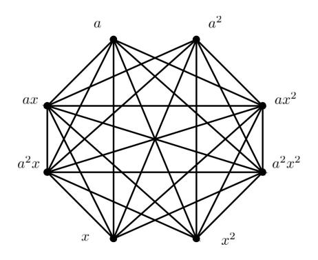
Figure 1. Heisenberg skeleton graph for p = 3.
In \(S_{\Gamma(G)}^M\) the only vertices with distance 2 are a with \(a^2\) and x with \(x^2\). Suppose without loss of generality that \(\psi(\{g,a\})=1\). The edge-disjoint paths for end vertices a and \(a^2\) are the following
\[\text{[rumus tidak dapat ditampilkan dengan baik — lihat PDF asli]}\]
And all the paths are given in 6.1.
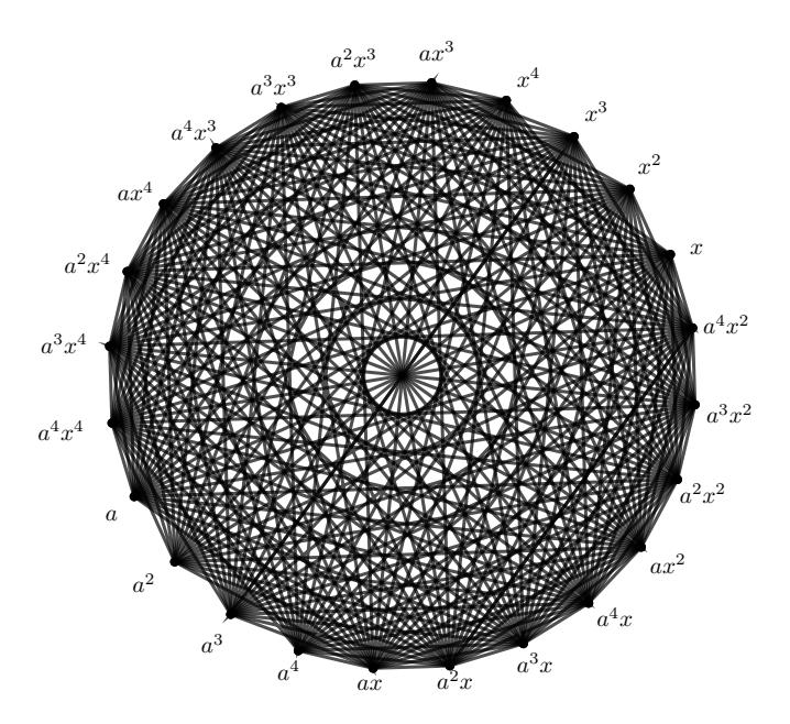
Figure 2. Heisenberg skeleton graph for p = 5.
Example 6.8. Let G be the Heisenberg group for p = 5 with presentation
\[\langle x, a, b | x^5 = a^5 = b^5 = 1, ab = ba, xax^{-1} = ab, xbx^{-1} = b \rangle.\]
We know that |G|=125, \(|G\setminus Z(G)|=120\) and |G/Z(G)|=25. Since [x,a]=b we have xa=bax, then xaZ=axZ. The graph 2 is the skeleton \(S^M_{\Gamma(G)}\) of G.
By 3.2 we know that we can found 5 edge-disjoint paths for any pair of vertices then, without loss of generality we give the 5 edge-disjoint paths for end vertices \(x, ax^2 \in S^M_{\Gamma(G)}\). By 1.3 we know that we need \(\left(\lfloor \frac{5}{2} \rfloor + 2\right)\)-color. The rainbow table is given below
\[\text{[rumus tidak dapat ditampilkan dengan baik — lihat PDF asli]}\]
Rainbow table for \(x \sim ax^2 \in S^M_{\Gamma(G)}\)
Then, the 5 edge-disjoin paths are given by:
We can give 4 paths with 4 colors. The rainbow and the 4 edge-disjoint paths with ends vertices \(x^4, x^3b^3\) are the following
\[\text{[rumus tidak dapat ditampilkan dengan baik — lihat PDF asli]}\]
If we note, we can not find 5 edge-disjoint paths with only 4 colors, for example, for the end vertices \(x^4b^4\) and \(x^3b^2\) we have the following paths:
| 1 | 6 F | ||
|---|---|---|---|
| Start with color 1 | Start with color 2 | ||
| \(x^4b^4 \stackrel{1}{\sim} a^3b^4 \stackrel{4}{\sim} x^3b^2\) | \(x^4b^4 \stackrel{2}{\sim} a^3 \stackrel{3}{\sim} x^3b^2\) | ||
| \(x^4b^4 \stackrel{1}{\sim} a^3b^4 \stackrel{3}{\sim} x^4b^2 \stackrel{2}{\sim} a^3b^3 \stackrel{4}{\sim} x^3b^2\) | \(x^4b^4 \stackrel{?}{\sim} a^3 \stackrel{3}{\sim} x^4b^3 \stackrel{4}{\sim} a^3b \stackrel{1}{\sim} x^3b^2\) | ||
| \(x^4b^4 \stackrel{1}{\sim} a^3b^4 \stackrel{4}{\sim} x^4 \stackrel{3}{\sim} a^3b^2 \stackrel{2}{\sim} x^3b^3\) | 2 | \(x^4b^4 \stackrel{2}{\sim} a^3 \stackrel{3}{\sim} x^4\) | \(b^3 \stackrel{1}{\sim} a^3 b^3 \stackrel{4}{\sim} x^3 b^2\) |
| \(x^4b^4 \stackrel{1}{\sim} a^3b^4 \stackrel{2}{\sim} x^3b^3 \stackrel{4}{\sim} a^3 \stackrel{3}{\sim} x^3b^3\) | 2 | \[x^4b^4 \stackrel{2}{\sim} a^3 \stackrel{1}{\sim} x^3\] | \[b \stackrel{3}{\sim} a^3 b^4 \stackrel{4}{\sim} x^3 b^2\] |
| Start with color 3 | Start with color \(x^4b^4 \stackrel{4}{\sim} a^3b^2\) | Start with color 4 from | |
| \[x^4b^4 \stackrel{4}{\sim} a^3b^3\] | |||
| \(x^4b^4 \stackrel{3}{\sim} a^3b \stackrel{1}{\sim} x^3b^2\) | \(x^4b^4 \stackrel{4}{\sim} a^3b^2\) | \(\stackrel{?}{\sim} x^3b^2\) | \(x^4b^4 \stackrel{4}{\sim} a^3b^3 \stackrel{1}{\sim} x^3b^4 \stackrel{3}{\sim}\) |
| \[x^3b^2 \stackrel{2}{\sim} x^3b^2\] | |||
| \(x^4b^4 \stackrel{3}{\sim} a^3b \stackrel{4}{\sim} x^4b^2 \stackrel{1}{\sim} a^3b^2 \stackrel{2}{\sim}\) | \(x^4b^4 \stackrel{4}{\sim} a^3b^2 \stackrel{3}{\sim} x^4 \stackrel{2}{\sim} a^3b \stackrel{1}{\sim}\) | \(x^4b^4 \stackrel{4}{\sim} a^3b^3 \stackrel{2}{\sim} x^3b^3 \stackrel{3}{\sim} x^3b \stackrel{1}{\sim}\) | |
| \(x^3b^2\) | \(x^3b^2\) | \(x^3b^2\) | |
| Color 3 can not came to color 4 | Color 4 can not came to color | Color \(x^4b^4 \stackrel{4}{\sim} a^3b^3\) can not | |
| \(a^3 \stackrel{3}{\sim} x^3 b^2\) | came to color \(a^3 \stackrel{3}{\sim} x^3 b^2\) | ||
Thus, we have not columns for do the rainbow path from \(x^4b^4 \stackrel{3}{\sim} a^3b\) to \(a^3b^3 \stackrel{4}{\sim} x^3b^2\)
\[\text{[rumus tidak dapat ditampilkan dengan baik — lihat PDF asli]}\]
Then, we can not find a path from \(x^4b^4\) to \(x^3b^2\) passes through \(a^3b\), because the last color from \(x^4b^4\) only can came to \(x^3b^2\) passes through \(a^3b\) and \(a^3b^2\). Then we need one more color.
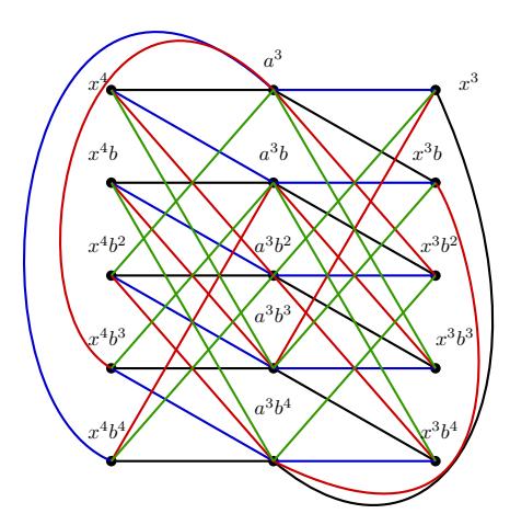
Figure 3. Graph in \(\Gamma(G)\)
\[\text{[rumus tidak dapat ditampilkan dengan baik — lihat PDF asli]}\]
Rainbow table for found the 5 edge-disjoin paths between \(x^4\) and \(x^3\)
With the given structure, we could ask about the meaning of d-coloring redundant as a generalization of [4]. For example, in Figure 3 we could considered a particular case of Turán graph with T(m|Z|,m).
Acknowledgements
This work was partially supported by CONACYT. We highly appreciate the valuable comments on our manuscript and the great editing.
References
- [1] A. Abdollahi, S. Akbari, and H. R. Maimani, Non-commuting graph of a group, J. Algebra 298 (2) (2006), 468–492.
- [2] G. Chartrand, G.L. Johns, K.A. McKeon, P. Zhang, The rainbow connectivity of a graph, Networks 54 (2009), 75–81.
- [3] M. R. Darafsheh, Groups with the same non-commuting graph, Discrete Appl. Math. 157 (2009), 833–837.
- [4] B. Demoen, N. Phuong-Lan, Graphs with coloring redundant edges, Electron. J. Graph Theory Appl. 4 (2) (2016), 223–230.
- [5] H. Deng, S. Balachandran, S. Elumalai, T. Mansour, Harary index of bipartite graphs Electron. J. Graph Theory Appl. 7 (2) (2019), 365–372.
- [6] B. H. Neumann, A problem of Paul Erdos on groups, ¨ J. Aust. Math. Soc. 21(Series A) (1976), 467–472.
- [7] A. Schrijver, Combinatorial Optimization: Polyhedra and Efficiency, Algorithms and Combinatorics, Volume 24, Springer-Verlag, Heidelberg, 2003.
- [8] F. Septyanto, K. A. Sugeng, Color code techniques in rainbow connection, Electron. J. Graph Theory Appl. 6 (2) (2018), 347–361.
- [9] Y. Wei, X. Ma and K. Wang, Rainbow connectivity of the non-commuting graph of a finite group, J. Algebra Appl. 15 (6) (2016), 1–8.
- [10] H. Whitney, Congruent graphs and the connectivity of graphs, American Journal of Matematics 54 (1) (1932), 150–168.