Christian Barrientos
Valencia College, Orlando, FL 32832, U.S.A.
chr barrientos@yahoo.com
Graceful labelings are an effective tool to find cyclic decompositions of complete graphs and complete bipartite graphs. The strongest kind of graceful labeling, the α-labeling, is in the center of the research field of graph labelings, the existence of an α-labeling of a graph implies the existence of several, apparently non-related, other labelings for that graph. Furthermore, graphs with α-labelings can be combined to form new graphs that also admit this type of labeling. The standard way to combine these graphs is to identify every vertex of a base graph with a vertex of another graph. These methods have in common that all the graphs involved, except perhaps the base, have the same size. In this work, we do something different, we prove the existence of an α-labeling of a tree obtained by attaching paths of different lengths to the vertices of a base path, in such a way that the lengths of the pendent paths form an arithmetic sequence with difference one, where consecutive vertices of the base path are identified with paths which lengths are consecutive elements of the sequence. These α-trees are combined in several ways to generate new families of α-trees. We also prove that these trees can be used to create unicyclic graphs with an α-labeling. In addition, we show that the pendent paths can be substituted by equivalent α-trees to produce new α-trees, obtaining in this manner a quite robust category of α-trees.
Keywords: α-labeling, graceful graph, unicyclic graph Mathematics Subject Classification : 05C78, 05C30
DOI: 10.5614/ejgta.2020.8.2.8
Received: 21 March 2020, Revised: 23 May 2020, Accepted: 18 June 2020.
1. Introduction
A difference vertex labeling of a graph G of size m is an injective mapping f from V (G) into a set S of nonnegative integers, such that every edge uv of G has assigned a weight defined by |f(u) − f(v)|. In this work the integer interval [a, b] is the set {a, a + 1, . . . , b}. The following labelings were introduced by Rosa [16]. The labeling f is called graceful when S = [0, m] and the set of induced weights is W = [1, m]. In this case, G is called a graceful graph. Let G be a bipartite graph and {A, B} be the natural bipartition of V (G), we refer to A and B as the stable sets of G where |A| = a and |B| = b. A bipartite labeling of G is an injection f : V (G) → [0, k] for which there is an integer λ, named the boundary value of f, such that f(u) ≤ λ < f(v) for every (u, v) ∈ A × B, that induces m different weights. From this definition we may conclude that k ≥ m; furthermore, the sets formed by the labels assigned by f on the vertices of A and B, denoted by LA and LB, are included in the interval [0, λ] and [λ + 1, k], respectively. If k = m, the function f is an α-labeling and G is an α-graph. Note that when f is an α-labeling of a tree such that f −1 (0) ∈ A, then its boundary value is λ = a − 1.
Suppose that f : V (G) → [0, m] is a graceful labeling of a graph G of size m. The function g : V (G) → [c, c + m], defined for every v ∈ V (G) and c ∈ Z as g(v) = c + f(v), is the shifting of f in c units. Note that this labeling preserves the weights induced by f. The function f : V (G) → [0, m], defined for every v ∈ V (G) as f(v) = m − f(v), is called the complementary labeling of f. This labeling not only preserves the weights induced by f, it also preserves their location, i.e., the weight of any edge of G is the same under both labelings.
Suppose now that f : V (G) → [0, m] is an α-labeling of a graph G of size m with boundary value λ. The function fr : V (G) → [0, m], defined for every v ∈ V (G) as fr(v) = λ − f(v) if f(v) ≤ λ, and fr(v) = m + λ + 1 − f(v) if f(v) > λ, is the reverse labeling of f. Note that fr is also an α-labeling of G with boundary value λ. Rosa [17] called this labeling the inverse of f. The function g : V (G) → {0, 1, . . . , m + d − 1}, defined for every v ∈ V (G) and d ∈ N as g(v) = f(v) if f(v) ≤ λ and g(v) = f(v) + d − 1 if f(v) > λ, is the d-graceful labeling of G obtained from f. Under the labeling g, we get LA = [0, λ] and LB = [λ + d, m + d − 1] and the set of induced weights is W = [d, m + d − 1]. This type of labeling was introduced independently by Maheo and Thuillier [12] and Slater [18].
When an α-labeling of a graph of size m is transformed into a d-graceful labeling shifted c units, LA = [c, c + λ], LB = [c + λ + d, c + m + d − 1] and W = [d, d + m − 1].
Suppose that G is graph of order m ≥ 4 and f is an α-labeling of G with boundary value λ. In the following table we show the labels of the vertices of G labeled 0, λ, λ + 1, and m by f under the labelings f, fr, and fr.
| u1 | u2 | u3 | u4 | |
|---|---|---|---|---|
| f | 0 | m | λ | λ + 1 |
| f | m | 0 | m − λ | m − λ − 1 |
| fr | λ | λ + 1 | 0 | m |
| fr | m − λ | m − λ − 1 | m | 0 |
Let G1 and G2 be two connected graphs. A graph G is said to be a vertex amalgamation of G1 and G2 if it is obtained by identifying a vertex of G1 with a vertex of G2. Vertex amalgamation is a widely used operation, which is the base of several of the techniques employed to build new graceful and/or α-graphs starting with two graphs that admit this type of labeling, see for example [2], [10], [13], and [19].
The following definition is an extension of the one given in [1]. Suppose that for each i ∈ [1, k], Gi is a connected graph with at least two vertices. Let ui , vi be two distinct vertices of Gi . A graph G obtained via vertex amalgamation of the Gi is called a chain graph if for each i ∈ [1, k − 1], the vertex vi of Gi is amalgamated with the vertex ui+1 of Gi+1.
In the next lemma we prove that if G1 and G2 are α-graphs, there exists a chain graph obtained with G1 and G2 that is also an α-graph.
Lemma 1.1. If G1 and G2 are α-graphs, then there is a vertex amalgamation of G1 and G2 that is an α-graph.
Proof. For each i = 1, 2, let Gi be a graph of size ni that admits an α-labeling fi with boundary value λi . The labeling of G1 is transformed into a (n2 + 1)-graceful labeling. In this way, LA1 = [0, λ1], LB1 = [λ1 + 1 + n2, n1 + n2], and W1 = [n2 + 1, n1 + n2]. The labeling of G2 is shifted λ1 + 1 units; thus, LA2 = [λ1 + 1, λ1 +λ2 + 1], LB2 = [λ1 +λ2 + 2, λ1 + 1 +n2], and W2 = [1, n2]. Therefore, both G1 and G2 have a vertex labeled λ1 + 1 + n2, and this is the only label repeated. In both cases, these vertices are in the stable sets containing the larger labels. Identifying these vertices, we get a vertex amalgamation of G1 and G2 which has an α-labeling. The boundary value of this labeling is λ = λ1 + λ2 + 1.
Graceful labelings were first introduced as a tool to attack Ringel-Kotzig Conjecture, which states that the complete graph K2n+1 can be decomposed into copies of any tree of size n. This conjecture is valid for every tree that admits a graceful labeling. The combination of these ideas generated what is called the Graceful Tree Conjecture, this conjecture says that every tree is graceful. Thus, graph labelings become a quite dynamic research area. Several articles devoted to the different types of labelings and their applications are published every year, being specially relevant those dedicated to labelings of trees. In this category we should mention the work of Mishra et al. [14], where the authors presented various families of trees of diameter 6 that admit a graceful labeling. The study of α-labelings not only is important within the research of difference vertex labelings and combinatorial design, this labeling has also influenced other types of labelings. For instance, Ichishima et al. [9] used the main characteristic of an α-labeling of a tree (that is, the vertices on each stable set are labeled with consecutive integers), in their work about consecutively super edge-magic labelings. Hence, the study of this kind of labeling not only has an intrinsic value, it also has implications in other areas of graph theory.
Vertex amalgamations of α-graphs play an important role in this work. In Section 2 we use them to assemble the paths P1, P2, . . . , Pn in such a way that the ith vertex of an extra copy of Pn is amalgamated with a leaf (or vertex of degree one) of Pi , producing what we call a triangular tree; we show that these trees admit an α-labeling. We conclude this section by proving that we can obtain another related family of α-trees if the paths P1, P2, . . . , Pn are replaced by Pk, Pk+1, . . . , Pk+n−1, where k is any positive integer other than one. In Section 3 we present three
ways to combine the \(\alpha\)-trees just obtained to produce new \(\alpha\)-trees that can also be described by way of vertex amalgamations. In Section 4 we exhibit a method that allows us to transform the \(\alpha\)-trees of the previous sections into \(\alpha\)-labeled unicyclic graphs. Section 5 is dedicated to describe a procedure that permits us to shift some edges of these \(\alpha\)-labeled trees without loosing in the process the main characteristic of the labeling. To show the relevance of this shifting technique, we count how many other \(\alpha\)-trees can be obtained from the \(\alpha\)-labeling of a triangular tree. We conclude our work in Section 6; there, we describe how the pendent paths of these \(\alpha\)-graphs can be replaced by other types of \(\alpha\)-trees.
We must note that all the graphs considered in this work are finite and simple, that is, with no multiple edges or loops. We use the standard notation and terminology used in [4] and [6].
2. Triangular Trees and \(\alpha\)-Labelings
Let \(v_1, v_2, \ldots, v_n\) be the consecutive vertices of \(P_n\), a triangular tree is obtained by amalgamating each \(v_i\) with a leaf (or vertex of degree 1) of \(P_i\). We denote this tree by \(T_n\) and refer to \(P_n\) as the base of \(T_n\). Note that \(T_n\) has size \(\frac{n^2+n-2}{2}\), which means that its order is a triangular number. We say that the first vertex of \(P_i\) is the leaf amalgamated with the vertex of \(P_n\). The earliest cases of \(T_n\) are shown in Figure 1 (see Figure 2 for a larger example).
The following lemma, due to Rosa [16], is of great relevance in this entire work, in particular in the first theorem, which is the cornerstone of this work.
Lemma 2.1. For every \(n \ge 1\), the path \(P_n\) is an \(\alpha\)-tree.
The \(\alpha\)-labeling of caterpillars given by Rosa [16], can be defined for paths in the following form. Assuming that \(v_1, v_2, \ldots, v_n\) are the consecutive vertices of the path \(P_n\), an \(\alpha\)-labeling of \(P_n\) is given by:
\[\phi(v_i) = \begin{cases} \frac{i-1}{2}, & \text{if } i \text{ is odd,} \\ n - \frac{i}{2}, & \text{if } i \text{ is even.} \end{cases}\]
The \(\alpha\)-labelings of the triangular trees in Figure 1 are going to be used to construct the \(\alpha\)-labelings of the larger cases. Since \(T_1 \cong K_1\), its \(\alpha\)-labeling is obtained assigning the label 0 to its vertex and it is omitted in this figure.
Theorem 2.1. For every \(n \ge 1\), the triangular tree \(T_n\) is an \(\alpha\)-tree.
Proof. We construct the \(\alpha\)-labeling of \(T_n\) in a recursive manner, utilizing the \(\alpha\)-labeling of \(T_{n-1}\) and the \(\alpha\)-labeling \(\phi\) of \(P_n\) given above. Recall that \(P_n\) is the path amalgamated with the last vertex of the base of \(T_n\).
Let f be the \(\alpha\)-labeling of \(T_{n-1}\) obtained by the recurrence. Suppose that f has boundary value \(\lambda\). The pendent path \(P_n\) is labeled using the function \(\phi\). The leaves of \(P_n\) have labels 0 and \(\frac{n}{2}\) when n is even, or 0 and \(\frac{n-1}{2}\) when n is odd. This labeling is shifted \(\lambda+1\) units; with this shifting the leaves are labeled \(\lambda+1\) and \(\frac{n}{2}+\lambda+1\) when n is even, or \(\lambda+1\) and \(\frac{n+1}{2}+\lambda\) when n is odd.
leaves are labeled \(\lambda+1\) and \(\frac{n}{2}+\lambda+1\) when n is even, or \(\lambda+1\) and \(\frac{n+1}{2}+\lambda\) when n is odd. Note that the last vertex of the base of \(T_{n-1}\) has label \(\lambda-\frac{n-2}{2}\) when n is even and label \(\lambda+1\) when n is odd. If f is transformed into a (n+1)-graceful labeling, the label \(\lambda+1\) becomes \(n+\lambda+1\) while the label \(\lambda-\frac{n-2}{2}\) remains the same.
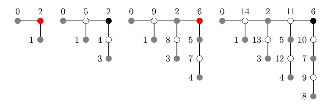
Figure 1. The smaller triangular trees with their \(\alpha\)-labeling
Now we connect, with an edge, this vertex with a leaf of \(P_n\). When n is even, we connect the vertex labeled \(\lambda - \frac{n-2}{2}\) of \(T_{n-1}\) with the leaf of \(P_n\) labeled \(\frac{n}{2} + \lambda + 1\). When n is odd, we connect the vertex labeled \(\lambda + 1\) of \(T_n - 1\) with the leaf of \(P_n\) labeled \(n + \lambda + 1\). Either way, the new edge has weight n.
Clearly, the new graph is \(T_n\). Since the labels on \(T_{n-1}\) are in \(L_A=[0,\lambda]\) and \(L_B=[\lambda+n+1,\frac{n^2+n-2}{2}]\), and the labels on \(P_n\) are in \([\lambda+1,\lambda+n]\), the labeling of \(T_n\) is injective. The weights on \(T_{n-1}\) form the interval \([n+1,\frac{n^2+n-2}{2}]\) and the new edges have weights in [1,n]. So, the edges of \(T_n\) have weights \(1,2,\ldots,\frac{n^2+n-2}{2}\). Since the labelings of both \(T_{n-1}\) and \(P_n\), prior to the connection between them, are bipartite and the labels of the vertices connected are not both larger than \(\lambda\), we conclude that the labeling of \(T_n\) is indeed an \(\alpha\)-labeling.
Remark 2.1. Note that the boundary value of \(T_n\) is \(\Lambda = (\frac{n-1}{2})^2 + n - 1\) when n is odd and \(\Lambda = (\frac{n}{2})^2 + \frac{n}{2} - 1\) when n is even.
In Figure 2 we show an example of this labeling for the case \(T_9\).
For each \(k \ge 1\), let \(T_{k,n}\) denote the tree obtained amalgamating to each vertex \(v_i\) of \(P_n\) a leaf of \(P_{k+i}\). In other terms, \(T_{k,n}\) is formed by deleting from the triangular tree \(T_{n+k}\) the subgraph induced by the vertices of \(T_k\). Hence the size of \(T_{k,n}\) is
\[\frac{(n+k)^2 + (n+k) - 2}{2} - \frac{k^2 + k - 2}{2} - 1\]
or equivalently,
\[\frac{n^2 + n(2k+1) - 2}{2}.\]
We refer to \(T_{k,n}\) as a truncated triangular tree. Once again, we refer to \(P_n\) as the base of \(T_{k,n}\).
Huang et al. [8] proved that all trees with at most four leaves are graceful. This implies that for \(1 \le n \le 4\), a graceful labeling of \(T_{k,n}\) is known. In the next theorem, we prove that for all \(n \ge 1\), the truncated triangular tree \(T_{k,n}\) is an \(\alpha\)-tree.
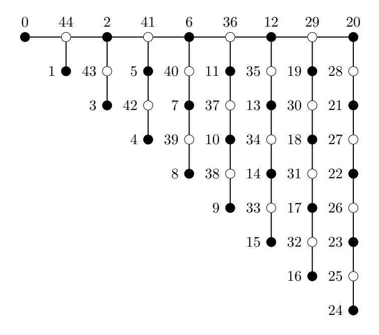
Figure 2. α-labeling of the triangular tree T9
Theorem 2.2. For all k ≥ 1 the truncated triangular tree Tk,n is an α-tree.
Proof. Suppose that both Tn+k and Tk have been labeled using the procedure described in Theorem 2.1. Thus, the boundary value of the α-labeling is the parameter Λ given in Remark 2.1. We proceed to delete from Tn+k the vertices of Tk and the edges incident to them. By construction, the remaining tree is Tk,n with a bipartite labeling, where the labels assigned form the interval [Λ + 1, (n+k) 2+(n+k)−2 2 ]. Note that the edges with the larger weights have been removed from Tn+k. By shifting −(Λ + 1) units the current labeling of Tk,n, we obtain an α-labeling of this truncated tree.
In Figure 5 we show an α-labeled unicyclic graph formed by connecting two copies of a truncated triangular tree. Essentially, the α-labeling of this tree, depicted with blue edges, is the labeling described in Theorem 2.2, so we can use that Figure 5 as an example of this theorem.
3. Combining Triangular Trees
As we mentioned earlier, α-graphs and α-trees in particular can be combined to generate other α-graphs. In this section we present three procedures to combine triangular and truncated triangular α-trees where the outcome is a new α-tree. In the first result we show that an α-tree is obtained when the last vertices of the bases of two copies of Tn are connected with an edge. This result can be encapsulated in a more general idea, presented in [2], to generate chain graphs. The second result follows the same scheme; now, the triangular trees connected can be different but they must have bases of even order. The last result uses the concept of edge amalgamation, introduced in [3], where any two triangular trees can be amalgamated.
Theorem 3.1. If T is the tree obtained with two copies of \(T_n\) by connecting with an edge the corresponding last vertices of their bases, then T is an \(\alpha\)-tree.
Proof. Since the size of \(T_n\) is \(\frac{n^2+n-2}{2}\), any tree formed by connecting with an edge two copies of \(T_n\) has size \(n^2+n-1\). Let f be the \(\alpha\)-labeling of \(T_n\) obtained in Theorem 2.1. Recall that f has boundary value \(\Lambda=(\frac{n-1}{2})^2+n-1\) when n is odd and \(\Lambda=(\frac{n}{2})^2+\frac{n}{2}-1\) when n is even. Initially, we label the first copy of \(T_n\) with the labeling f, once this is done, we transform f into a \((\frac{n^2+n+2}{2})\)-graceful labeling. In this way, \(L_{A_1}=[0,\Lambda], L_{B_1}=[\Lambda+\frac{n^2+n+2}{2},\frac{n^2+n-2}{2}+\frac{n^2+n+2}{2}-1]=[\Lambda+\frac{n^2+n}{2}+1,n^2+n-1],\) and \(W_1=[\frac{n^2+n+2}{2},n^2+n-1].\) On the other side, the starting labeling of the second copy of \(T_n\), is the complementary of the reverse of f, i.e., \(\overline{f_r}\). Thus, \(L_{A_2}=[\frac{n^2+n-2}{2}-\Lambda,\frac{n^2+n-2}{2}],\) \(L_{B_2}=[0,\frac{n^2+n-2}{2}-\Lambda-1],\) and \(W_2=[1,\frac{n^2+n-2}{2}].\) Once this labeling is in place, we proceed to shift it \(\Lambda+1\) units. As a consequence, we get \(L_{B_2}=[1,\frac{n^2+n-2}{2}]\) and \(L_{A_2}=[\frac{n^2+n-2}{2}+1,\frac{n^2+n-2}{2}+\Lambda+1]=[\frac{n^2+n-2}{2},\Lambda+\frac{n^2+n}{2}].\)
Now we want to find the label of the last vertex in the base of \(T_n\). We consider two cases depending of the parity of n. When n is odd, its label under f is \(\Lambda - \frac{n-1}{2}\). This implies that its label in the first copy of \(T_n\) is still \(\Lambda - \frac{n-1}{2}\) and on the second copy it is \(\Lambda + 1 + \frac{n^2-1}{2}\). Hence, when we connect both copies, using these vertices, the new edge has weight \(\frac{n^2+n-2}{2}+1\); therefore, T is an \(\alpha\)-tree.
When n is even, the label of the last vertex of the base of \(T_n\) under the labeling f is \(\Lambda+1\). Then its label on the first copy is \(\Lambda+1+\frac{n^2+n}{2}\), and on the second copy is \(\Lambda+1\). As in the odd case, the weight of the new edge, that connects the two copies, is \(\Lambda+1+\frac{n^2+n}{2}-\Lambda-1=\frac{n^2+n}{2}=\frac{n^2+n-2}{2}+1\), and T is an \(\alpha\)-tree.
In the case where n is even, the argument used in this last proof can be extended even further. We do not need two copies of the same triangular tree, we just need two triangular trees which bases have even order. Indeed, suppose that m and n are even. Let \(T^1 \cong T_m\) and \(T^2 \cong T_n\). For i=1,2, let \(f_i\) be the \(\alpha\)-labeling of \(T^i\) and \(\Lambda_i\) be its boundary value. Thus, the last vertex of the base of \(T^i\) has label \(\Lambda_i+1\). The labeling of \(T^1\) is transformed into a \((\frac{n^2+n-2}{2}+2)\)-graceful labeling, as we did in the proof above. Then, the last vertex in the base of \(T^1\) has now label \(\Lambda_1 + \frac{n^2+n+2}{2}\). To connect the two trees we need an edge with weight \(\frac{n^2+n}{2}\). So we need to label the last vertex on the base of \(T^2\) with \(\Lambda_1+1\). This is always possible because the labeling \(\overline{f_r}\) of \(T^2\) places the label 0 on that vertex, which becomes \(\Lambda_1+1\) after the labeling is shifted conveniently. Thus, we have proven the following result.
Theorem 3.2. Let m and n be even numbers. If T is the tree obtained with two triangular trees \(T_m\) and \(T_n\) by connecting with an edge the corresponding last vertices of their bases, then T is an \(\alpha\)-tree.
These ideas can be iterated to form trees like the one shown in Figure 3, which is obtained with the tree T formed with two copies of \(T_4\) connected using Lemma 1.1 twice. The first time the lemma is used to construct a tree G with \(G_1 = T\) and \(G_2 = P_2\), and the second time to \(G_1 = G\) and \(G_2 = T\). Moreover, since the last vertex on the base of the new tree T is labeled \(\Lambda + 1\), it can
be amalgamated with the vertex, of an α-labeled caterpillar (or any α-tree), with the largest label. The other extreme of this caterpillar can be amalgamated with any triangular tree or any tree of the one discussed above.
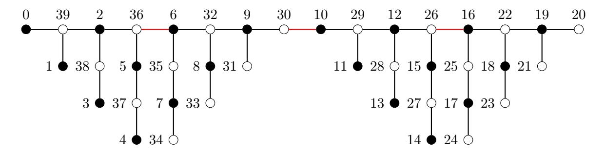
Figure 3. α-tree formed with multiple copies of T4
In [3] we introduced the concept of edge amalgamation of graphs. Let F and G be two graphs of positive size. The graph H obtained by identifying an edge of F with an edge of G is called an edge amalgamation of F and G. The edge of H shared by F and G is named link. The order of H is |V (H)| = |V (F)| + |V (G)| − 2 and its size is |E(H)| = |E(F)| + |E(G)| − 1. This operation was introduced as a tool to produce a new α-graph, H, when a specifically selected edge from each of the α-graphs, F and G, is used to be the link between them. In the next theorem, we use the edge amalgamation of triangular trees with the same goal, that is, to create new and different α-labeled trees.
Theorem 3.3. If T is the result of the edge amalgamation of two triangular trees, where the edges amalgamated are the first edges of the corresponding bases, then T is an α-tree.
Proof. For i = 1, 2, let Tni be a triangular tree. Suppose that fi is the α-labeling of Tni , obtained in Theorem 2.1 and that Λi is its boundary value. The final labeling of Tni is obtained in two steps. When i = 1, fi is transformed into its reverse and this labeling is transformed into a ( n 2 2+n2−2 2 ) graceful labeling. For i = 2, f2 is transformed into its complementary labeling, which is finally shifted Λ + 1 units. Thus, the only repeated labels are those on the end-vertices of the first edges of the corresponding bases.
In Figure 4 we show an example of an α-tree constructed using Theorem 3.3 on two trees that result of the edge amalgamation of T4 with T8 and T4 with T5. The links are the red edges, the edge use to connect these edge amalgamations is the green edge between T8 and T4.
4. Pendent Paths on α-Cycles
The study of graceful labelings of unicyclic graphs has received some attention during the last decades, several papers can be found in the specialized literature. In [5], Ichishima et al., provided a pair of methods to build unicyclic graceful graphs. Basically, their methods can be described as the vertex amalgamation of α-labeled trees of the same size one per vertex of the cycle Cn. In this
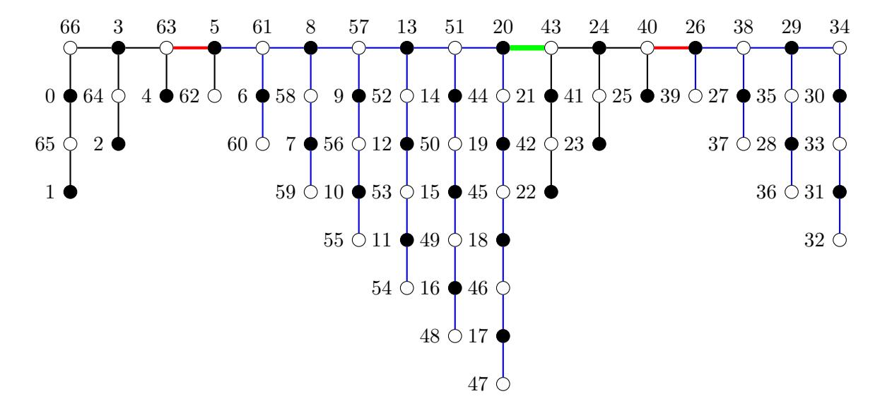
Figure 4. \(\alpha\)-labeling of a path with pendent paths formed via edge amalgamation
section, we study how the triangular trees or some derived trees can be used to build \(\alpha\)-labeled unicyclic graphs. The process is a small variation of the procedure described in Theorem 3.1. This technique differs from the ideas in [5] because the paths that we are attaching to the vertices of the cycle have different sizes. In Section 6, we study some conditions, that when are satisfied by an \(\alpha\)-labeled graph, allow us to replace these paths by, what we called, equivalent \(\alpha\)-trees, which increases substantially the number of known gracefully labeled unicyclic graphs.
Theorem 4.1. Suppose that \(T^1\) and \(T^2\) are two copies of the triangular tree \(T_n\) or the truncated tree \(T_{k,n}\), where both n and k are even. Let \(u_i\) and \(v_i\) be the first and last vertices of the base of \(T^i\). If G is the unicyclic graph obtained by connecting with an edge \(u_1\) to \(u_2\) and \(v_1\) to \(v_2\), then G is an \(\alpha\)-graph.
Proof. Suppose that both \(T^1\) and \(T^2\) have been labeled using the method in Section 2. Since n is even, the last vertex of the base of \(T^i\) has label \(\Lambda+1\); the first vertex of its base has label 0 when \(T^i\cong T_n\) and also when \(T^i\cong T_{k,n}\) because k is even.
If \(T^i\) has size q, the unicyclic graph G has size 2q+2. We start by transforming the labeling of \(T^1\) into a (q+3)-graceful labeling. Thus, \(L_{A_1}=[0,\Lambda]\), \(L_{B_1}=[\Lambda+q+3,2q+2]\), \(W_1=[q+3,2q+2]\), the label of \(u_1\) is still 0, and the label of \(v_1\) is now \(\Lambda+q+3\). The labeling of \(T^2\) is transformed into its complementary reverse labeling, shifted \(\Lambda+2\) units. In this case, \(L_{A_2}=[q+2,\Lambda+q+2]\), \(L_{B_2}=[\Lambda+2,q+1]\), \(W_2=[1,q]\), the label of \(u_2\) is q+2, and the new label of \(v_2\) is \(\Lambda+2\).
Hence, when \(u_1\) and \(u_2\) are connected by an edge, this edge has weight q+2. When \(v_1\) and \(v_2\) are connected with an edge, this edge has weight \((\Lambda + q + 3) - (\Lambda + 2) = q + 1\). Therefore, the weights on the edges of G are \(1, 2, \ldots, 2q + 2\) and G is an \(\alpha\)-graph.
In Figure 5 we show an example of a unicyclic \(\alpha\)-graph which labeling follows the steps presented in Theorem 4.1. In its construction, we used two copies of the truncated tree \(T_{4,4}\).
Figure 5. α-labeled unicyclic graph formed with two copies of the truncated tree T4,8
Now that we know how to connect triangular or truncated triangular trees to produce α-labeled unicyclic graphs, we explore other alternatives to extend this technique. Recall that, independently of the parity of n, the first vertex of Tn is labeled 0 and that when we constructed the tree T, in Theorem 3.1, the labeling of the second copy of Tn is a shifting of the complementary reverse labeling of the one used on the first copy; this implies that the last vertex of the base of T is labeled Λ + 1. The relative position of these two labels, 0 and Λ + 1, is the critical condition for the veracity of Theorem 4.1; this condition is not present when the order of the base in Tn or Tk,n is odd. Luckily, as we just said, the tree T, from Theorem 3.1, places the labels 0 and Λ + 1 on vertices of the base located in the opposite extremes, which means that we can apply the argument of Theorem 4.1, using two trees like the one in Theorem 3.1, to form a new α-labeled unicyclic graph. We omit the proof of this new result because is basically the same that the proof of the previous theorem.
Theorem 4.2. Suppose that T and T are two trees obtained using Theorem 3.1. Let ui and vi be the first and last vertex of the base of T i . If G is the unicyclic graph obtained by connecting with an edge u1 to u2 and v1 to v2, then G is an α-graph
We can go even further, the same principle can be applied to prove that any unicyclic graph formed with r > 1 copies of the tree T is an α-graph. In Figure 6 we show an example of this extended construction for a tree formed using three copies of a tree T formed, using Theorem 3.1, with two copies of the triangular tree T3.
Figure 6. Alpha-labeling of a cycle with pendent paths
5. Shifting Edges in Triangular Trees
In this section we explore how an edge of the base of the \(\alpha\)-labeled triangular tree \(T_n\) can be replaced by a new edge connecting two vertices of consecutive pendent paths to produce a new \(\alpha\)-labeled tree that is not isomorphic to \(T_n\).
Theorem 5.1. For \(n \ge 3\) and each \(i \in [2, n-1]\), there exist \(x_i, x_{i+1} \in V(T_n)\), not in its base, such that the edge \(v_i v_{i+1}\) of the base can be replaced by the edge \(x_i x_{i+1}\) to produce a new \(\alpha\)-tree.
Proof. Suppose that the triangular tree \(T_n\) has been labeled using the \(\alpha\)-labeling f given in Theorem 2.1. Recall that the labeling of each pendent path in \(T_n\) is a modification of the \(\alpha\)-labeling \(\phi\) associated to Lemma 2.1, and that this modification does not change its bipartite characteristic. This implies that when d is an even number, the label of any vertex w on the a pendent path amalgamated with the vertex v of the base, located at distance d from v, is \(f(w) = f(v) + \frac{d}{2}\).
Let i be any element of [2, n-1], \(v_iv_{i+1}\) be an edge on the base of \(T_n\), and \(d \le i\) be a positive even number. Then, there exists a vertex \(x_i\) in the pendent path amalgamated with \(v_i\) and a vertex \(x_{i+1}\) in the pendent path amalgamated with \(v_{i+1}\), such that \(\operatorname{dist}(v_i, x_i) = \operatorname{dist}(v_{i+1}, x_{i+1}) = d\). Thus,
\[|f(x_{i+1}) - f(x_i)| = |(f(v_{i+1}) + d/2) - (f(v_i) + d/2)| = |f(v_{i+1}) - f(v_i)|.\]
Therefore, we can delete the edge \(v_i v_{i+1}\) from \(T_n\) and insert the new edge \(x_i x_{i+1}\) to produce a new tree with an \(\alpha\)-labeling.
Suppose now that \(i \in [2, n-1]\) is even. By the construction of the \(\alpha\)-labeling f of \(T_n\), we know that the label of \(v_i\) is larger than the labels of its neighbors; in particular, \(f(v_i) > f(v_{i+1})\). Moreover, if \(w_i\) and \(w_{i+1}\) are the vertices of the pendent paths, adjacent to \(v_i\) and \(v_{i+1}\), respectively, then \(f(w_i) = f(v_{i+1}) - 1\) and \(f(w_{i+1}) = f(v_i) - 1\). This implies that if the edge \(v_i v_{i+1}\) is deleted from \(T_n\) and the vertices \(w_i\) and \(w_{i+1}\) are connected, this new edge has the same weight that the deleted edge. But the distance between \(v_i\) and \(w_i\), or \(v_{i+1}\) and \(w_{i+1}\) is one. Consequently, \(\operatorname{dist}(v_i, x_i) = \operatorname{dist}(v_{i+1}, x_{i+1})\) does not need to be even to have a new edge \(x_i x_{i+1}\) with the same weight that \(v_i v_{i+1}\) with a final result of an \(\alpha\)-labeled tree.
Clearly, every edge on the base of \(T_n\), except \(v_1v_2\) can be replaced by a "parallel" line and multiple edges of the base can be replaced at the same time with exactly the same effect, that
is, obtaining a new \(\alpha\)-labeled tree. In Figure 7 we show an example of tree obtained from the triangular tree \(T_9\) shown if Figure 2, the red edges connect vertices at an odd distance from the base. Furthermore, this replacement of edges can be applied to any of the trees presented here because the \(\alpha\)-labeling of them is originated in the labeling of \(T_n\).
Figure 7. \(\alpha\)-labeling of a tree obtained by shifting some edges of the base of \(T_9\)
This flexibility to replace some edges of \(T_n\), allows us to construct a big number of \(\alpha\)-labeled, non-isomorphic trees. In the next theorem, we calculate the number of non-isomorphic trees obtained from \(T_n\).
Theorem 5.2. The number of non-isomorphic trees that can be constructed by replacing any subset of edges of the base of \(T_n\) is given by:
\[a(n) = \begin{cases} 2^{\frac{n-1}{2}} \left(\frac{n-1}{2}!\right)^2, & \text{if } n \text{ is odd}, \\ 2^{\frac{n-2}{2}} \cdot \frac{n}{2} \left(\frac{n-2}{2}!\right)^2, & \text{if } n \text{ is even}. \end{cases}\]
Proof. Recall that the base of \(T_n\) has consecutive vertices \(v_1, v_2, \ldots, v_n\) and that \(v_i\) has been amalgamated with the path of order i. In addition, the edge \(v_i v_{i+1}\) can be replaced by the edge \(x_i x_{i+1}\), where these vertices are in the pendent path amalgamated to \(v_i\) and \(v_{i+1}\), respectively. Besides, \(\operatorname{dist}(v_i, x_i) = \operatorname{dist}(v_{i+1}, x_{i+1})\) and this distance must be even when i is odd.
Suppose first that n is even. The amount of odd and even numbers in [1, n-1] is \(\frac{n-1}{2}\). If i is odd, the number of ways to choose \(x_i\) is \(1 \cdot 2 \cdot 3 \cdot \ldots \cdot \frac{n-1}{2} = \frac{n-1}{2}!\). If i is even, this number is
\(2 \cdot 4 \cdot 6 \cdot \ldots \cdot (n-1) = 2^{\frac{n-1}{2}} \cdot \frac{n-1}{2}!\). Therefore,
\[a(n) = 2^{\frac{n-1}{2}} \left( \frac{n-1}{2}! \right)^2.\]
Suppose now that n is even. The amount of odd numbers in [1, n-1] is \(\frac{n}{2}\) but the amount of even numbers is \(\frac{n-2}{2}\). If i is odd, the number of ways to choose \(x_i\) is \(\frac{n}{2}\)!. When i is even, this number is \(2 \cdot 4 \cdot 6 \cdot \ldots \cdot (n-2) = 2^{\frac{n-2}{2}} \cdot \frac{n-2}{2}\)!.
Consequently,
\[a(n) = 2^{\frac{n-2}{2}} \cdot \frac{n-2}{2}! \cdot \frac{n}{2}! = 2^{\frac{n-2}{2}} \cdot \frac{n}{2} \left(\frac{n-2}{2}!\right)^2.\]
In the following table we present the first values of a(n) and in Figure 8 we show the sixteen non-isomorphic trees obtained with \(T_5\). Note that the majority of these trees are not caterpillars, this means that the majority of the trees that we are generating in this way are not necessarily known to be graceful or admitting an \(\alpha\)-labeling.
| n | 1 | 2 | 3 | 4 | 5 | 6 | 7 | 8 | 9 | 10 | 11 | 12 |
|---|---|---|---|---|---|---|---|---|---|---|---|---|
| a(n) | 1 | 1 | 2 | 4 | 16 | 48 | 288 | 1152 | 9216 | 46,080 | 460,800 | 2,764,800 |
Table 1. Number of \(\alpha\)-trees built from the triangular tree \(T_n\)
Figure 8. All 16 non-isomorphic trees obtained from \(T_5\)
6. Substituting the Pendent Paths
For i=1,2, let \(T_i\) be an \(\alpha\)-tree of size m with stable sets \(A_i\) and \(B_i\). We say that \(T_1\) and \(T_2\) are equivalent if at least one of the two following conditions holds: (i) \(|A_1| = |A_2|\) or (ii) \(|A_1| = |B_2|\). Without loss of generality we assume that for any two equivalent \(\alpha\)-trees, \(T_1\) and \(T_2\), \(|A_1| = |A_2|\). Since \(T_i\) is an \(\alpha\)-tree, there exists an \(\alpha\)-labeling of \(T_i\) with boundary value \(\lambda = |A_i| - 1\). In the next lemma we prove that under some necessary conditions we can replace an induce subtree of a gracefully labeled graph with any equivalent tree.
Lemma 6.1. Let G be a gracefully labeled graph, and S and T be two non-isomorphic equivalent α-trees, such that S is an induced subgraph of G. If the induced labeling of S is a shifting of a d-graceful labeling, then a graceful graph G0 is obtained by replacing the edges of S in G by the edges of T.
Proof. Suppose that G is a graceful graph and f is a graceful labeling of G. Let S and T be two equivalent trees of size m, where S is an induced subgraph of G such that f restricted to the vertices of S is a shifting in c units of a d-graceful labeling. Since S and T are equivalent, there exists an α-labeling of T such that when it is transformed into a d-graceful labeling shifted c units, we get that LAS = LAT and LBS = LBT . Thus, we can delete from G all the edges of S and replace them with the edges of T, because the stable sets of S can be matched with the stable sets of T and for each weight w ∈ [d, d + m − 1], both trees have an edge of weight w. Hence, once all the edges of S have been replaced with the edges of T, the new graph G0 has a graceful labeling for the reason that the labels have not been altered by the replacements and the new edges have the same weights that the ones replaced.
Note that when the labeling of G is an α-labeling, so it is the labeling of G0 .
As we mentioned before, a well-known family of α-trees is the one formed by caterpillars. Harary and Schwenk [7] proved that the number of caterpillars of order n is given by c(n) = 2 n−4 + 2b n−4 2 . The entry T(n − 3, k) of Losanitsch's triangle, sequence A034851 in OEIS, gives us the number of caterpillars of order n and diameter k + 2, where 0 ≤ k ≤ n−3. Several of these caterpillars are equivalent to the path Pn. Using the list of trees of order up to 12 given in [15], we counted these caterpillars; in the table given below we show the number c(n) of caterpillars equivalent to Pn, including Pn itself, as well as the number t(n) of α-trees that can be formed from the triangular tree Tn, when any number of the pendent paths are substituted by equivalent caterpillars.
| n | 1 | 2 | 3 | 4 | 5 | 6 | 7 | 8 | 9 | 10 | 11 | 12 |
|---|---|---|---|---|---|---|---|---|---|---|---|---|
| c(n) | 1 | 1 | 1 | 1 | 2 | 3 | 6 | 7 | 19 | 23 | 66 | 71 |
| t(n) | 1 | 1 | 1 | 1 | 2 | 6 | 36 | 252 | 4788 | 110,124 | 7,268,184 | 516, 041,064 |
Table 2. Number of caterpillars equivalent to Pn and α-trees built from the triangular tree Tn
In the previous sections we showed several graphs obtained by attaching pendent paths to the vertices of a graph called the base, in sections 2 and 3, this base is a path and in Section 4 it is an α-cycle. In all these cases, the labeling of each pendent path is a shifting of a d-graceful labeling generated with the α-labeling φ of the path. Therefore, these paths can be replaced with an equivalent α-tree and the resulting graph is indeed an α-graph. In the Introduction we showed that, in general, in an α-graph G, there are at least four vertices where the labels 0 or m can be located by an α-labeling of the graph. Under some conditions, that depend on the automorphisms of the graph, there are only two of these vertices. In our constructions, the label of the vertex of the pendent path amalgamated with the base is either the smallest or the largest label assigned to
the path. As a consequence of Lemma 6.1 and the corresponding results on the previous sections, we have the following corollaries.
Corollary 6.1. Let \(T_n\) be a triangular tree. Any tree obtained from \(T_n\) by replacing any number of pendent paths with equivalent trees is an \(\alpha\)-tree.
Corollary 6.2. Let \(T_{k,n}\) be a truncated triangular tree. Any tree obtained from \(T_{k,n}\) by replacing any number of pendent paths with equivalent trees is an \(\alpha\)-tree.
Corollary 6.3. Let G be any unicyclic graph from Theorem 4.1. Any unicyclic graph obtained from G by replacing any number of pendent paths with equivalent trees is an \(\alpha\)-graph.
As an example of the kind of \(\alpha\)-graphs generated using Lemma 6.1 in combination with the \(\alpha\)-trees previously constructed, we show in Figure 9 an \(\alpha\)-tree obtained from a tree produced applying Theorem 3.1 to two copies of the truncated tree \(T_{6,4}\).
In [17], Rosa proved that with only one exception (the central vertex of \(P_5\)), there exists an \(\alpha\)-labeling of \(P_m\) that assigns the label 0 (consequently the label m-1) to any of its vertices. This implies that the amalgamation of the vertex \(v_i\) of \(P_n\) and the pendent path \(P_i\) can be done with any of the vertices of \(P_i\), not only with a leaf, except in the case where \(P_i \cong P_5\) and its central vertex. A couple of consequences of this property of \(P_m\) are the following:
Corollary 6.4. Let \(n \equiv 0 \pmod{4}\) and \(v_1, v_2, \ldots, v_n\) be the consecutive vertices of \(C_n\). A unicyclic \(\alpha\)-graph is obtained by identifying each \(v_i\) with any vertex of a path, where the paths amalgamated to \(v_i\) and \(v_{n+1-i}\) have order i and neither \(v_5\) nor \(v_{n-4}\) are amalgamated with the central vertex of \(P_5\).
Note that the amount of unicyclic graphs that can be generated with this procedure is substantial. Using Pólya's enumeration theorem we found that the number a(m) of non-isomorphic unicyclic graphs built using as base the cycle \(C_{4m}\) is given by \(\frac{1}{2}((m!)^4 + (m!)^2)\). Just to appreciate the magnitude of this number, in the following table we show the first values of a(m).
| m | 1 | 2 | 3 | 4 | 5 | 6 | |
|---|---|---|---|---|---|---|---|
| a(m) | 1 | 10 | 666 | 166,176 | 103,687,200 | 134,369,539,200 | |
Corollary 6.5. Suppose that \(v_1, v_2, \ldots, v_n\) are the consecutive vertices of \(P_n\). An \(\alpha\)-tree is obtained by identifying each \(v_i\) with the central vertex of \(P_{2i+5}\).
7. Conclusions
Through the several sections of this article, we have seen different alternatives to use \(\alpha\)-labeled trees to build new and larger \(\alpha\)-graphs. Even when \(\alpha\)-labelings are the most restrictive of the labelings introduced by Rosa [16], they are the most generous, not only in the sense described by López and Muntaner-Batle [11], but also in the manner they are used here. In despite of the large amount of \(\alpha\)-graphs that can be formed with the, quite simple, triangular trees, we must emphasize
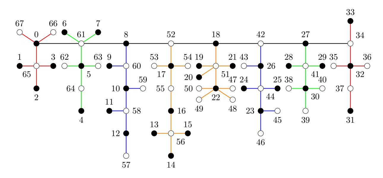
Figure 9. α-labeling of a path with pendent α-trees
the fact that when the induced labeling of the (pendent) paths satisfies certain conditions, these paths can be substituted with equivalent α-trees. Clearly, this idea works with any graph not only paths. Thus, in the search of graceful labelings of more intricate graphs, eventually some subgraphs can be replaced by easier structures which α-labelings are known.
Acknowledgement
I would like to thank the anonymous referee for his/her valuable comments, suggestions, and attentive reading of the manuscript.
References
- [1] C. Barrientos, Graceful labelings of chain and corona graphs, Bull. Inst. Combin. Appl., 34 (2002) 17–26.
- [2] C. Barrientos, On graceful chain graphs, Util. Math., 78 (2009) 55–64.
- [3] C. Barrientos and S. Minion, Alpha labelings of snake polyominoes and hexagonal chains, Bull. Inst. Combin. Appl., 74 (2015) 73–83.
- [4] G. Chartrand and L. Lesniak, Graphs & Digraphs 4th ed. CRC Press, Boca Raton, FL 33487 (2005).
- [5] R. Figueroa-Centeno, R. Ichishima, F. Muntaner-Batle, and A. Oshima, Gracefully cultivating trees on a cycle, Electron. Notes Discrete Math., 48 (2015) 143–150.
- [6] J.A. Gallian, A dynamic survey of graph labeling, Electron. J. Combin. (2019), #DS6.
- [7] F. Harary and A.J. Schwenk, The number of caterpillars, Discrete Math., 6 (1973), 359–365.
- [8] C. Huang, A. Kotzig, and A. Rosa, Further results on tree labellings, Util. Math., 21c (1982) 31–48.
- [9] R. Ichishima, F.A. Muntaner-Batle, and A. Oshima, The consecutively super edge-magic deficiency of graphs and related concepts, Electron. J. Graph Theory Appl., 8 (1) (2020), 181–194.
- [10] K.M. Koh, D.G. Rogers, and T. Tan, Products of graceful trees, Discrete Math., 31 (1980) 279–292.
- [11] S.C. Lopez and F.A. Muntaner-Batle, ´ Graceful, Harmonious and Magic Type Labelings: Relations and Techniques, Springer, Cham, 2017.
- [12] M. Maheo and H. Thuillier, On d-graceful graphs, Ars Combin., 13 (1982) 181–192.
- [13] M. Mavronicolas and L. Michael, A substitution theorem for graceful trees and its applications, Discrete Math., 309 (2009) 3757–3766.
- [14] D. Mishra, S.K. Rout, and P.C. Nayak, Some new graceful generalized classes of diameter six trees, Electron. J. Graph Theory Appl., 5 (1) (2017), 181–194.
- [15] R.C. Read and R.J. Wilson, An Atlas of Graphs, Oxford University Press, Oxford, England, 1998.
- [16] A. Rosa, On certain valuations of the vertices of a graph, Theory of Graphs (Internat. Symposium, Rome, July 1966), Gordon and Breach, N. Y. and Dunod Paris (1967) 349–355.
- [17] A. Rosa, Labelling snakes, Ars Combin., 3 (1977) 67–74.
- [18] P.J. Slater, On k-graceful graphs, Proc. of the 13th S.E. Conf. on Combinatorics, Graph Theory and Computing, (1982) 53–57.
- [19] R. Stanton and C. Zarnke, Labeling of balanced trees, Proc. 4th Southeast Conf. Combin., Graph Theory, Comput., (1973) 479–495.