Doost Ali Mojdeha , Seyed Reza Musawib , Esmaeil Nazari Kiashic
Department of Mathematics, University of Tafresh, Tafresh, Iran
damojdeh@umz.ac.ir, r musawi@shahroodut.ac.ir, nazari.esmaeil@gmail.com
Let G be a graph and k be a positive integer. A vertex set D is called a k-distance dominating set of G if each vertex of G is either in D or at a maximum distance k from some vertex of D. k-distance domination number of G is the minimum cardinality among all k-distance dominating sets of G. In this note we give upper bounds on the k-distance domination number of a connected bipartite graph, and improve some results have been given like Theorems 2.1 and 2.7 in [Tian and Xu, A note on distance domination of graphs, Australasian Journal of Combinatorics, 43 (2009), 181-190].
Keywords: domination, k-distance domination, connected bipartite graph
Mathematics Subject Classification: 05C69, 05C12
DOI: 10.5614/ejgta.2020.8.2.11
1. Introduction
We refer the reader to [9] for terminology and notation on graph theory not given here. In a simple graph G with vertex set V (G) = V and edge set E(G) = E, the order and the size of G is denoted by n = |V (G)| and m = |E(G)|, respectively. The open neighborhood of a vertex v is defined as N(v) := {u ∈ V : uv ∈ E}, and the set N[v] = N(v) ∪ {v} is called the closed
Received: 1 July 2017, Revised: 5 April 2020, Accepted: 14 June 2020.
aDepartment of Mathematics, University of Mazandaran, Babolsar, Iran
bFaculty of Mathematical Sciences, Shahrood University of Technology, P.O. Box 36199-9516, Shahrood, Iran &
cDepartment of Mathematics, University of Tafresh, Tafresh, Iran
neighborhood of v. Similarly, the set N(S) = ∪v∈SN(v) is called the open neighborhood of a set S ⊆ V and the set N[S] = N(S) ∪ S is the closed neighborhood of S. For a vertex v ∈ V , the degree of v is degG(v) = deg(v) = |N(v)|. δ = δ(G) and ∆ = ∆(G) denote the minimum degree and maximum degree, respectively, among all vertices of G. For a vertex v ∈ V , the set Nk(v) = {u : d(u, v) ≤ k and u 6= v} is called the open k-neighborhood of v. In the other words, Nk(v) is the set of all vertices in within distance k of v. The set Nk[v] = Nk(v) ∪ {v} is said to be the closed k-neighborhood of v.
A set D ⊆ V is a dominating set if every vertex in V − D has a neighbor in D. The minimum cardinality among all dominating sets of G is called the domination number of G and is denoted by γ(G). A vertex set K ⊆ V is a k-distance dominating set if every vertex in V − K is within distance k of some vertex in K. In the other words, if K ⊆ V is a k-distance dominating set of G, then Nk[K] = V . The k-distance domination number of G, γk(G), is the minimum cardinality among all k-distance dominating sets in G, for further see, [3, 4, 5, 8]. The kth power graph of G is a new graph with V (Gk ) = V (G) and two vertices x, y ∈ V (Gk ) are adjacent in Gk if dG(x, y) ≤ k. Note that γk(G) equals to γ(Gk ), where Gk is the kth power graph of G, see [2, 4, 6, 7].
2. Previous known results
Tian and Xu [7] studied k-distance domination number in graphs. They have proved the following results.
Theorem 2.1 (Tian and Xu [7], Theorem 2.1). Let V = {1, 2, · · · , n} be the vertex set of a connected graph G. Then γk(G) ≤ min (p1,p2,··· ,pn)∈(0,1)n Pn i=1 pi + (1 − pi) Π j∈Nk(i) (1 − pj ) where pi ∈ (0, 1) is the probability of existence of the vertex i in a random subset of V .
Then they considered connected bipartite graph.
Lemma 2.1 (Tian and Xu [7], Lemma 2.5). Let G be a connected bipartite graph with bipartition V1 and V2, where |Vj | = nj and δj = min{deg(v) : v ∈ Vj}, for j = 1, 2. For any vertex v ∈ V1 with Nk[v] 6= V ,
\[|N_k(v) \cap V_1| \ge (\lceil k/6 \rceil - 1)(\delta_2 + 1),\tag{1}\]
\[|N_k(v) \cap V_2| \ge \lceil k/6 \rceil (\delta_1 + 1) - 1. \tag{2}\]
Similarly, for any vertex v ∈ V2 with Nk[v] 6= V ,
\[|N_k(v) \cap V_1| \ge \lceil k/6 \rceil (\delta_2 + 1) - 1, \tag{3}\]
\[|N_k(v) \cap V_2| \ge (\lceil k/6 \rceil - 1)(\delta_1 + 1). \tag{4}\]
Let G be a connected bipartite graph. It is said to be perfect if δ1δ2 > 1, n2[M(δ2 + 1) − 1] > n1[(M − 1)(δ1 + 1) + 1] and n1[M(δ1 + 1) − 1] > n2[(M − 1)(δ2 + 1) + 1], where M = dk/6e. A simple calculation shows that a connected bipartite graph is perfect if and only if n1 − n2δ2 < M[n1(δ1 + 1) − n2(δ2 + 1)] < n1δ1 − n2. As a consequence of Lemma 2.1 and Theorem 2.1, Tian and Xu obtained the following.
Theorem 2.2 (Tian and Xu [7], Theorem 2.7). Let G be a perfect bipartite graph and
\[0 < p_1 = \frac{[(M-1)(\delta_1+1)+1]\ln u - [M(\delta_1+1)-1]\ln v}{(2M-1)(\delta_1\delta_2-1)} < 1\]
\[0 < p_2 = \frac{[(M-1)(\delta_2+1)+1] \ln v - [M(\delta_2+1)-1] \ln u}{(2M-1)(\delta_1\delta_2-1)} < 1,\]
where u = n2[M(δ2+1)−1]−n1[(M−1)(δ1+1)+1] n1(2M−1)(δ1δ2−1) and v = n1[M(δ1+1)−1]−n2[(M−1)(δ2+1)+1] n2(2M−1)(δ1δ2−1) . Then
\[\text{[rumus tidak dapat ditampilkan dengan baik — lihat PDF asli]}\]
where M = dk/6e.
In this manuscript we improve Theorem 2.2 via improving the Lemma 2.1.
3. Main results
In order to improve Theorem 2.2, we first improve Lemma 2.1.
Lemma 3.1. Let G be a connected bipartite graph with bipartition V1 and V2, where |Vj | = nj and δj = min{deg(v) : v ∈ Vj}, for j = 1, 2. Then (i) For any vertex v ∈ V1 with Nk[v] 6= V ,
\[|N_k(v) \cap V_1| \ge \lceil (k-1)/4 \rceil \max\{2, \delta_2\} + 2\lfloor k/4 \rfloor - \lfloor k/2 \rfloor, \tag{5}\]
\[|N_k(v) \cap V_2| \ge \delta_1 + (\lceil k/4 \rceil - 1) \max\{2, \delta_1\} + \lfloor (k-1)/2 \rfloor - 2\lfloor (k-1)/4 \rfloor.\] (6)
Furthermore, (5) and (6), improve (1) and (2), repectively.
(ii) For any vertex v ∈ V2 with Nk[v] 6= V ,
\[|N_k(v) \cap V_1| \ge \lceil k/4 \rceil \max\{2, \delta_2\} + \lfloor (k-1)/2 \rfloor - 2\lfloor (k-1)/4 \rfloor, \tag{7}\]
\[|N_k(v) \cap V_2| \ge \lceil (k-1)/4 \rceil \max\{2, \delta_1\} + 2\lfloor k/4 \rfloor - \lfloor k/2 \rfloor. \tag{8}\]
Furthermore, (7) and (8) improve (3) and (4), respectively.
Proof. Let G be a connected bipartite graph with bipartition V1 and V2, where |Vj | = nj and δj = min{deg(v) : v ∈ Vj}, for j = 1, 2. For any vertex v and any integer l with 1 ≤ l ≤ k, let Xl(v) = {u ∈ V |d(v, u) = l}. It is obvious that Nk(v) = X1(v) ∪ X2(v) ∪ · · · ∪ Xk(v). Furthermore, X1(v), X2(v),...,and . . . , Xk(v) are pairly disjoint.
(i) Let v ∈ V1 be a vertex with Nk[v] 6= V . Observe that X1(v) ∪ X3(v) ∪ · · · ∪ X2b(k+1)/2c−1(v) ⊆ V2, X2(v) ∪ X4(v) ∪ · · · ∪ X2bk/2c(v) ⊆ V1, and
\[N_k(v) \cap V_1 = \bigcup_{m=1}^{\lfloor k/2 \rfloor} X_{2m}(v), \ N_k(v) \cap V_2 = \bigcup_{m=1}^{\lfloor (k+1)/2 \rfloor} X_{2m-1}(v).\]
Thus, \[|N_k(v) \cap V_1| = \sum_{m=1}^{\lfloor k/2 \rfloor} |X_{2m}(v)|\] and \(|N_k(v) \cap V_2| = \sum_{m=1}^{\lfloor (k+1)/2 \rfloor} |X_{2m-1}(v)|\). Since \(N_k[v] \neq V\),
there exists a vertex u such that d(v, u) > k. Therefore, there exists a path, P := vx1x2 . . . u of length of at least k + 1. For l = 1, 2, · · · , k, Xl(v) 6= ∅, because xl ∈ Xl(v). Moreover, if l is odd, then deg(xl) ≥ max{2, δ2}, because xl ∈ V2; while if l is even, then deg(xl) ≥ max{2, δ1}, because xl ∈ V1. We continue with two following claims.
Claim 1. |X2(v)| ≥ max{2, δ2} − 1 ≥ δ2 − 1.
To see this, note that since x1 ∈ X1(v) ⊆ V2, we have |X2(v)| = deg(x1) − 1. Since deg(x1) ≥ max{2, δ1}, we find that |X2(v)| ≥ max{2, δ2} − 1, as desired.
Claim 2. For 2 ≤ l ≤ k − 1, |Xl−1(v)| + |Xl+1(v)| ≥ deg(xl).
To see this, note that for 2 ≤ l ≤ k − 1, we have N1(xl) = N(xl) ⊆ Xl−1(v) ∪ Xl+1(v), since xl ∈ Xl(v).
By Claim 2, |X4m(v)| + |X4m+2(v)| ≥ deg(x4m+1) for every m = 1, 2, ..., b bk/2c−1 2 c. To compute |Nk(v) ∩ V1|, we discuss on bk/2c−1 2 which may be an integer or not.
First we assume that bk/2c−1 2 is an integer. Hence,
\[\begin{split} |N_k(v) \cap V_1| &= \sum_{m=1}^{\lfloor k/2 \rfloor} |X_{2m}(v)| = |X_2(v)| + \sum_{m=2}^{\lfloor k/2 \rfloor} |X_{2m}(v)| \\ &= |X_2(v)| + \sum_{m'=1}^{(\lfloor k/2 \rfloor - 1)/2} (|X_{4m'}(v)| + |X_{4m'+2}(v)|) \\ &\geq \max\{2, \delta_2\} - 1 + \sum_{m'=1}^{(\lfloor k/2 \rfloor - 1)/2} \max\{2, \delta_2\} \quad (by \ Claims \ 1 \ and \ 2). \end{split}\]
Thus, |Nk(v)∩V1| ≥ (bk/2c + 1) max{2, δ2}/2 − 1 and a simple calculation shows that (bk/2c + 1) max{2, δ2}/2 − 1 = d(k − 1)/4e max{2, δ2} + 2bk/4c − bk/2c, as desired.
Next we assume that bk/2c−1 2 is not an integer. Hence,
\[\begin{split} |N_k(v) \cap V_1| &= \sum_{m=1}^{\lfloor k/2 \rfloor} |X_{2m}(v)| = |X_2(v)| + \sum_{m=2}^{\lfloor k/2 \rfloor - 1} |X_{2m}(v)| + |X_{2\lfloor k/2 \rfloor}| \\ &= |X_2(v)| + \sum_{m'=1}^{(\lfloor k/2 \rfloor - 2)/2} (|X_{4m'}(v)| + |X_{4m'+2}(v)|) + |X_{2\lfloor k/2 \rfloor}| \\ &\geq \max\{2, \delta_2\} - 1 + \sum_{m'=1}^{(\lfloor k/2 \rfloor - 2)/2} \max\{2, \delta_2\} + 1 \quad (by \ Claims \ 1 \ and \ 2). \end{split}\]
Therefore, we have |Nk(v) ∩ V1| ≥ bk/2c max{2, δ2}/2 and a simple calculation shows that bk/2c max{2, δ2}/2 = d(k − 1)/4eδ2 + 2bk/4c − bk/2c, as desired.
Consequently, inequality (5) holds. We next prove inequality (6). Since deg(v) ≥ δ1 and N(v) = X1(v) ⊆ V2, we find that |X1(v)| ≥ δ1.
From Claim 2, we can easily see that \(|X_{4m-1}(v)| + |X_{4m+1}(v)| \ge \deg(x_{4m}) \ge \max\{2, \delta_1\}\) for every \(m=1,2,...,\lfloor\frac{k-1}{4}\rfloor\). We discuss on \(\frac{\lfloor (k+1)/2\rfloor}{2}\) which may be an integer or not.
First we assume that \(\frac{\lfloor (k+1)/2 \rfloor}{2}\) is an integer. Hence,
\[\begin{split} |N_k(v) \cap V_2| &= \sum_{m=1}^{\lfloor (k+1)/2 \rfloor} |X_{2m-1}(v)| = |X_1(v)| + \sum_{m=2}^{\lfloor (k+1)/2 \rfloor} |X_{2m-1}(v)| \\ &= |X_1(v)| + \sum_{m'=1}^{\lfloor (k+1)/2 \rfloor/2-1} (|X_{4m'-1}(v)| + |X_{4m'+1}(v)|) + |X_{2\lfloor (k+1)/2 \rfloor-1}(v)| \\ &\geq \delta_1 + \sum_{m'=1}^{\lfloor (k+1)/4 \rfloor-1} \max\{2, \delta_1\} + 1 \quad (by \ Claim \ 2). \end{split}\]
Thus, \(|N_k(v) \cap V_2| \ge \delta_1 + (\lfloor (k+1)/4 \rfloor - 1) \max\{2, \delta_1\} + 1\). Now a simple calculation shows that \(\delta_1 + (\lfloor (k+1)/4 \rfloor - 1) \max\{2, \delta_1\} + 1 = \delta_1 + (\lceil k/4 \rceil - 1) \max\{2, \delta_1\} + \lfloor (k-1)/2 \rfloor - 2\lfloor (k-1)/4 \rfloor\) as desired.
Next we assume that \(\frac{\lfloor (k+1)/2 \rfloor}{2}\) is not an integer. Hence,
\[|N_k(v) \cap V_2| = \sum_{m=1}^{\lfloor (k+1)/2 \rfloor} |X_{2m-1}(v)| = |X_1(v)| + \sum_{m=2}^{\lfloor (k+1)/2 \rfloor} |X_{2m-1}(v)|\] \[= |X_1(v)| + \sum_{m'=1}^{(\lfloor (k+1)/2 \rfloor - 1)/2} (|X_{4m'-1}(v)| + |X_{4m'+1}(v)|)\] \[\geq \delta_1 + \sum_{m'=1}^{\lfloor (k-1)/4 \rfloor} \max\{2, \delta_1\} \quad (by \ Claim \ 2).\]
Thus, \(|N_k(v) \cap V_2| \ge \delta_1 + \lfloor (k-1)/4 \rfloor \max\{2, \delta_1\}\). Now a simple calculation shows that \(\delta_1 + \lfloor (k-1)/4 \rfloor \max\{2, \delta_1\} = \delta_1 + (\lceil k/4 \rceil - 1) \max\{2, \delta_1\} + \lfloor (k-1)/2 \rfloor - 2\lfloor (k-1)/4 \rfloor\) as desired.
We next show that inequality 5 is an improvement of inequality 1. We will show that:
\[\lceil \frac{k-1}{4} \rceil \max\{2, \delta_2\} + 2\lfloor \frac{k}{4} \rfloor - \lfloor \frac{k}{2} \rfloor \ge (\lceil \frac{k}{6} \rceil - 1)(\delta_2 + 1)\]
It is obvious that if \(\delta_2=1\), then the left side of the above inequality is \(2\lceil\frac{k-1}{4}\rceil+2\lfloor\frac{k}{4}\rfloor-\lfloor\frac{k}{2}\rfloor=\lfloor\frac{k}{2}\rfloor\) and the right side is \(2(\lceil\frac{k}{6}\rceil-1)\), and clearly \(2\lceil\frac{k-1}{4}\rceil+2\lfloor\frac{k}{4}\rfloor-\lfloor\frac{k}{2}\rfloor=\lfloor\frac{k}{2}\rfloor\geq 2(\lceil\frac{k}{6}\rceil-1)\) for \(k\geq 1\). Thus assume that \(\delta_2\geq 2\). We show that
\[(\lceil \frac{k-1}{4} \rceil - \lceil \frac{k}{6} \rceil + 1) \delta_2 \ge \lceil \frac{k}{6} \rceil - 1 - 2 \lfloor \frac{k}{4} \rfloor + \lfloor \frac{k}{2} \rfloor\]
for \(k \ge 1\). Let \(L = (\lceil \frac{k-1}{4} \rceil - \lceil \frac{k}{6} \rceil + 1)\delta_2\) and \(R = \lceil \frac{k}{6} \rceil - 1 - 2\lfloor \frac{k}{4} \rfloor + \lfloor \frac{k}{2} \rfloor\). Now, we show that \(L \ge R\). Let k = 12p + q, where \(1 \le q \le 12\). Then
\[L = (\lceil \frac{k-1}{4} \rceil - \lceil \frac{k}{6} \rceil + 1)\delta_2 = p\delta_2 + (\lceil \frac{q-1}{4} \rceil - \lceil \frac{q}{6} \rceil + 1)\delta_2.\]
\[R = \lceil \frac{k}{6} \rceil - 1 - 2 \lfloor \frac{k}{4} \rfloor + \lfloor \frac{k}{2} \rfloor = 2p + \lceil \frac{q}{6} \rceil - 1 - 2 \lfloor \frac{q}{4} \rfloor + \lfloor \frac{q}{2} \rfloor.\]
Since \(\delta_2 \geq 2\), we have \(p\delta_2 \geq 2p\). So we need to show that \((\lceil \frac{q-1}{4} \rceil - \lceil \frac{q}{6} \rceil + 1)\delta_2 \geq \lceil \frac{q}{6} \rceil - 1 - 2\lfloor \frac{q}{4} \rfloor + \lfloor \frac{q}{2} \rfloor\). Since \(1 \leq q \leq 12\), we show this by Table 1.
| q | 1 | 2 | 3 | 4 | 5 | 6 | 7 | 8 | 9 | 10 | 11 | 12 |
|---|---|---|---|---|---|---|---|---|---|---|---|---|
| \(\left(\left\lceil \frac{q-1}{4}\right\rceil - \left\lceil \frac{q}{6}\right\rceil + 1\right)\delta_2.\) | 0 | \(\delta_2\) | \(\delta_2\) | \(\delta_2\) | \(\delta_2\) | \(2\delta_2\) | \(\delta_2\) | \(\delta_2\) | \(\delta_2\) | \(2\delta_2\) | \(2\delta_2\) | \(2\delta_2\) |
| \(\lceil \frac{q}{6} \rceil - 1 - 2 \lfloor \frac{q}{4} \rfloor + \lfloor \frac{q}{2} \rfloor \rceil\) | 0 | 1 | 1 | 0 | 0 | 1 | 2 | 1 | 1 | 2 | 2 | 1 |
Table 1.
Thus, inequality (5) is an improvement of inequality (1). Next, we show that inequality (6) is an improvement of inequality (2). We will show that:
\[\delta_1 + (\lceil k/4 \rceil - 1) \max\{2, \delta_1\} + |(k-1)/2| - 2|(k-1)/4| \ge \lceil k/6 \rceil (\delta_1 + 1) - 1\]
If \(\delta_1 = 1\), then the above inequality becomes \(1 + 2(\lceil k/4 \rceil - 1) + \lfloor (k-1)/2 \rfloor - 2\lfloor (k-1)/4 \rfloor = \lceil k/2 \rceil \ge 2\lceil \frac{k}{6} \rceil - 1\) which is valid for any \(k \ge 1\). Thus we assume that \(\delta_1 \ge 2\). It is sufficient to show that
\[\left( \left\lceil \frac{k}{4} \right\rceil - \left\lceil \frac{k}{6} \right\rceil \right) \delta_1 \ge \left\lceil \frac{k}{6} \right\rceil - 1 - \left\lfloor \frac{k-1}{2} \right\rfloor + 2 \left\lfloor \frac{k-1}{4} \right\rfloor\]
for \(k \geq 1\). Let \(L = (\lceil \frac{k}{4} \rceil - \lceil \frac{k}{6} \rceil) \delta_1\) and \(R = \lceil \frac{k}{6} \rceil - 1 - \lfloor \frac{k-1}{2} \rfloor + 2 \lfloor \frac{k-1}{4} \rfloor\). Thus, we need to show that \(L \geq R\). Let k = 12p + q, where \(1 \leq q \leq 12\). Hence,
\[L = (\lceil \frac{k}{4} \rceil - \lceil \frac{k}{6} \rceil) \delta_1 = p \delta_1 + (\lceil \frac{q}{4} \rceil - \lceil \frac{q}{6} \rceil) \delta_1.\] \[R = \lceil \frac{k}{6} \rceil - 1 - \lfloor \frac{k-1}{2} \rfloor + 2 \lfloor \frac{k-1}{4} \rfloor = 2p + \lceil \frac{q}{6} \rceil - 1 - \lfloor \frac{q-1}{2} \rfloor + 2 \lfloor \frac{q-1}{4} \rfloor.\]
| q | 1 | 2 | 3 | 4 | 5 | 6 | 7 | 8 | 9 | 10 | 11 | 12 |
|---|---|---|---|---|---|---|---|---|---|---|---|---|
| \((\lceil \frac{q}{4} \rceil - \lceil \frac{q}{6} \rceil) \delta_1\) | 0 | 0 | 0 | 0 | \(\delta_1\) | \(\delta_1\) | 0 | 0 | \(\delta_1\) | \(\delta_1\) | \(\delta_1\) | \(\delta_1\) |
| \(\left\lceil \left\lceil \frac{q}{6} \right\rceil - 1 - \left\lfloor \frac{q-1}{2} \right\rfloor + 2 \left\lfloor \frac{q-1}{4} \right\rfloor \right\rceil\) | 0 | 0 | -1 | -1 | 0 | 0 | 0 | 0 | 1 | 1 | 0 | 0 |
Table 2.
Since \(\delta_1 \geq 2\), we have \(p\delta_1 \geq 2p\). Therefore, it is sufficient to show that \((\lceil \frac{q}{4} \rceil - \lceil \frac{q}{6} \rceil)\delta_1 \geq \lceil \frac{q}{6} \rceil - 1 - \lfloor \frac{q-1}{2} \rfloor + 2\lfloor \frac{q-1}{4} \rfloor\). We do this in Table 2, since \(1 \leq q \leq 12\). Thus (6) is an improvement of (2).
The proof of part (ii), (i.e. (7) and (8)) is similar and straightforward, and therefore is omitted.
Theorem 3.1. If G is a bipartite graph and k is a positive integer, then
\[\gamma_k(G) \leq \min_{(p_1, p_2) \in (0, 1)^2} h^*(p_1, p_2),\] where \[h^*(p_1, p_2) = n_1 p_1 + n_1 e^{-p_1 (A_{11} + 1) - p_2 A_{12}} + n_2 p_2 + n_2 e^{-p_1 A_{21} - p_2 (A_{22} + 1)}\] \[A_{11} = \lceil (k - 1)/4 \rceil \max\{2, \delta_2\} + 2\lfloor k/4 \rfloor - \lfloor k/2 \rfloor\] \[A_{12} = \delta_1 + (\lceil k/4 \rceil - 1) \max\{2, \delta_1\} + \lfloor (k - 1)/2 \rfloor - 2\lfloor (k - 1)/4 \rfloor\] \[A_{21} = \delta_2 + (\lceil k/4 \rceil - 1) \max\{2, \delta_2\} + \lfloor (k - 1)/2 \rfloor - 2\lfloor (k - 1)/4 \rfloor\] \[A_{22} = \lceil (k - 1)/4 \rceil \max\{2, \delta_1\} + 2\lfloor k/4 \rfloor - \lfloor k/2 \rfloor\]
This bound improve the given bound in Theorem 2.2.
Proof. By Theorem 2.1, we have
\[\gamma_k(G) \le \min_{(p_1, p_2) \in (0, 1)^2} \left( \sum_{v \in V_1} \left[ p_1 + (1 - p_1)^{|N_k(v) \cap V_1| + 1} (1 - p_2)^{|N_k(v) \cap V_2|} \right] + \sum_{v \in V_2} \left[ p_2 + (1 - p_1)^{|N_k(v) \cap V_1|} (1 - p_2)^{|N_k(v) \cap V_2| + 1} \right] \right).\]
By Lemma 3.1, we have
\[\gamma_k(G) \leq \min_{(p_1, p_2) \in (0, 1)^2} \left( \sum_{v \in V_1} \left[ p_1 + (1 - p_1)^{A_{11} + 1} (1 - p_2)^{A_{12}} \right] + \sum_{v \in V_2} \left[ p_2 + (1 - p_1)^{A_{21}} (1 - p_2)^{A_{22} + 1} \right] \right)\] \[\leq \min_{(p_1, p_2) \in (0, 1)^2} \left( \left[ n_1 p_1 + n_1 (1 - p_1)^{A_{11} + 1} (1 - p_2)^{A_{12}} \right] + \left[ n_2 p_2 + n_2 (1 - p_1)^{A_{21}} (1 - p_2)^{A_{22} + 1} \right] \right)\] \[\leq \min_{(p_1, p_2) \in (0, 1)^2} \left( n_1 p_1 + n_1 e^{-p_1 (A_{11} + 1) - p_2 A_{12}} + n_2 p_2 + n_2 e^{-p_1 A_{21} - p_2 (A_{22} + 1)} \right).\]
That is γk(G) ≤ min (p1,p2)∈(0,1)2 h ∗ (p1, p2). To show that our bound is an improvement of the bound given in Theorem 2.2, note that by Lemma 3.1 one can easily see that h ∗ (p1, p2) ≤ h(p1, p2), since exp(−x) is a decreasing function.
Example 3.1. It remains to show that there are perfect graphs that our bound is better than the older one. For this purpose, let G be a connected bipartite graph with n1 = n2 = n 2 , δ1 = δ2 = δ ≥ 2, and k = 4m + 1 with m = 1, 2, 3, · · · . We can easily see that the graph is perfect. Now we have A11 = A22 = mδ, A12 = A21 = (m + 1)δ and
\[h^*(p_1, p_2) = \frac{n}{2} [p_1 + p_2 + e^{-p_1(m\delta+1) - p_2(m+1)\delta} + e^{-p_1(m+1)\delta - p_2(m\delta+1)}].\]
By using of calculus method, we see that the unique minimum of \(h^*\) occurs at
\[p_1 = p_2 = \frac{\ln[(2m+1)\delta + 1]}{(2m+1)\delta + 1},\]
since \(0 < p_1 = p_2 < 1\), we have \(\min_{\substack{(p_1,p_2) \in (0,1)^2}} h^*(p_1,p_2) = n(\frac{1+\ln[(2m+1)\delta+1]}{(2m+1)\delta+1})\). By calculus, we note that the function \(f(x) = \frac{1+\ln x}{x}\) is decreasing on interval \((1,\infty)\) and also we have \((2m+1)\delta+1 \geq (2\lceil k/6\rceil-1)(\delta+1)\), thus the new bound refinements the bound in Theorem 2.2.
3.1. Minimizing \(h^*(p_1, p_2)\)
In this part of paper we wish to minimize \(h^*(p_1, p_2)\). For this purpose, we consider two different cases and we use calculation methods.
3.1.1. k is even
In this case we will show that either \(h^*\) hasn't local extremum or it has infinitely local minimum on \((0,1)^2\). However \(h^*\) has local minimum on closed unit square \([0,1]^2\), thus we extend the domain of \(h^*\) into \([0, 1]^2\).
Before introducing our main results, we explain an observation in calculus:
Observation 3.1. Consider the function \(f(x) = \frac{a + \ln x}{x}\) where x > 0 and a > 0. f has a unique maximum in \(x = e^{1-a} \le e\) thus \(f(x) \le f(e^{1-a}) = e^{a-1}\). Now, if a < 1, then f(x) < 1 for all x > 0.
Our main result in this states is:
Theorem 3.2. If k is an even integer, \(\delta_1, \delta_2 \geq 2\) and \(T = \max\{\frac{nA_{12}}{n_2}, \frac{nA_{21}}{n_1}\}\), in each of three cases
- (i) \(\frac{nA_{12}}{nA_{12}} = \frac{nA_{21}}{nA_{21}}\)
\[\begin{array}{l} (i) \ \frac{nA_{12}}{n_2} = \frac{nA_{21}}{n_1} \\ (ii) \ \frac{nA_{12}}{n_2} < \frac{nA_{21}}{n_1} \ and \ \frac{1}{A_{21}} \ln \frac{nA_{21}}{n_1} < 1 \\ (iii) \ \frac{nA_{12}}{n_2} > \frac{nA_{21}}{n_1} \ and \ \frac{1}{A_{12}} \ln \frac{nA_{12}}{n_2} < 1 \\ we \ have \ \inf_{(p_1,p_2)\in(0,1)^2} h^*(p_1,p_2) = \min_{(p_1,p_2)\in[0,1]^2} h^*(p_1,p_2) = n(\frac{1+\ln T}{T}). \end{array}\]
Proof. If we assume that \(k \stackrel{4}{\equiv} 0\), then
\[A_{11} = k\delta_2/4\], \(A_{12} = k\delta_1/4 + 1\), \(A_{21} = k\delta_2/4 + 1\), \(A_{22} = k\delta_1/4\)
and if \(k \stackrel{4}{\equiv} 2\), then
\[A_{11} = (k+2)\delta_2/4 - 1\], \(A_{12} = (k+2)\delta_1/4\), \(A_{21} = (k+2)\delta_2/4\), \(A_{22} = (k+2)\delta_1/4 - 1\).
Thus, in both cases we have \(A_{11} + 1 = A_{21}\) and \(A_{22} + 1 = A_{12}\), and therefore,
\[h^*(p_1, p_2) = n_1 p_1 + n_2 p_2 + n e^{-p_1 A_{21} - p_2 A_{12}}.\]
To minimize \(h^*(p_1,p_2)\), using partial differential, we have \(h^*_{p_1}=n_1-nA_{21}e^{-p_1A_{21}-p_2A_{12}}\) and \(h^*_{p_2}=n_2-nA_{12}e^{-p_1A_{21}-p_2A_{12}}\). From \(h^*_{p_1}=0\), we obtain that \(e^{-p_1A_{21}-p_2A_{12}}=\frac{n_1}{nA_{21}}\), and so \(p_1A_{21}+p_2A_{12}=\ln\frac{nA_{21}}{n_1}\). Likewise, from \(h^*_{p_2}=0\), we obtain \(p_1A_{21}+p_2A_{12}=\ln\frac{nA_{12}}{n_2}\). (i) If \(\frac{A_{21}}{n_1}=\frac{A_{12}}{n_2}\), then for all \((p_1,p_2)\) with \(p_1A_{21}+p_2A_{12}=\ln\frac{nA_{12}}{n_2}=\ln\frac{nA_{21}}{n_1}\), we have:
\[h^*(p_1, p_2) = n_1 p_1 + n_2 p_2 + n e^{-p_1 A_{21} - p_2 A_{12}} = \frac{n_1}{A_{21}} (p_1 A_{21} + p_2 A_{12}) + n e^{-p_1 A_{21} - p_2 A_{12}}\]\[= \frac{n_1}{A_{21}} \ln \frac{n A_{21}}{n_1} + n e^{-\ln \frac{n A_{21}}{n_1}} = \frac{n_1}{A_{21}} (1 + \ln \frac{n A_{21}}{n_1}).\]
Therefore, \(h^*\) is constant for all \((p_1,p_2)\) with \(p_1A_{21}+p_2A_{12}=\ln\frac{nA_{12}}{n_2}=\ln\frac{nA_{21}}{n_1}\) (See Figure 1). Note that two points \((0,\frac{1}{A_{12}}\ln\frac{nA_{12}}{n_2})\) and \((\frac{1}{A_{21}}\ln\frac{nA_{21}}{n_1},0)\) are located on the line \(p_1A_{21}+p_2A_{12}=\ln\frac{nA_{12}}{n_2}=\ln\frac{nA_{21}}{n_1}\) and by Observation 3.1, we have \(0<\min\{\frac{1}{A_{12}}\ln\frac{nA_{12}}{n_2},\frac{1}{A_{21}}\ln\frac{nA_{21}}{n_1}\}<1\) because \(0<\min\{\ln\frac{n}{n_2},\ln\frac{n}{n_1}\}<1\).
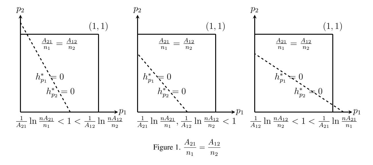
Thus the minimum of \(h^*(p_1,p_2)\) is \(\frac{n_1}{A_{21}}(1+\ln\frac{nA_{21}}{n_1})\), and note that it happens for every pairs \((p_1,p_2)\in(0,1)^2\), satisfying \(h^*_{p_1}=h^*_{p_2}=0\). Now letting \(T=\frac{nA_{21}}{n_1}=\frac{nA_{12}}{n_2}\), we obtain that \(\min_{p_1,p_2}h^*(p_1,p_2)=n(\frac{1+\ln T}{T})\), as desired.
If \(\frac{A_{21}}{n_1} \neq \frac{A_{12}}{n_2}\), then \(p_1A_{21} + p_2A_{12} = \ln \frac{nA_{21}}{n_1}\) and \(p_1A_{21} + p_2A_{12} = \ln \frac{nA_{12}}{n_2}\) are two distinct parallel lines in the \(p_1p_2\)-coordinate system. Thus, \(h^*\) has no extremum in \((0,1)^2\) but it has an infimum value in \((0,1)^2\). For this purpose we seek the extremum of \(h^*\) in \([0,1]^2\). Observe that the line \(p_1A_{21} + p_2A_{12} = \ln \frac{nA_{21}}{n_1}\) intersects the \(p_1\)-axis in \(M_1 = (\frac{1}{A_{21}} \ln \frac{nA_{21}}{n_1}, 0)\) and \(p_2\)-axis in \(N_1 = (0, \frac{1}{A_{12}} \ln \frac{nA_{21}}{n_1})\). Similarly, the line \(p_1A_{21} + p_2A_{12} = \ln \frac{nA_{12}}{n_2}\) intersects the \(p_1\)-axis in \(M_2 = (\frac{1}{A_{21}} \ln \frac{nA_{12}}{n_2}, 0)\) and \(p_2\)-axis in \(N_2 = (0, \frac{1}{A_{12}} \ln \frac{nA_{12}}{n_2})\). Moreover, let \(Q_1 = (1, 0)\) and \(Q_2 = (0, 1)\). (ii) \(\frac{nA_{12}}{n_2} < \frac{nA_{21}}{n_1}\) and \(\frac{1}{A_{21}} \ln \frac{nA_{21}}{n_1} < 1\) we prove that the minimum of \(h^*\) occurs in \(M_1\). For each point \((p_1, p_2)\) in unit square \([0, 1]^2\) there is a unique point \((p_1', p_2)\) on segments \(M_1N_1\) or \(N_1Q_2\)
(dotted segments in Figure 2) such that \(h^*(p_1',p_2) \leq h^*(p_1,p_2)\). Hence, the minimum of \(h^*\) occurs on \(M_1N_1 \cup N_1Q_2\). Also, there is a unique point \((p_1,p_2')\) on segments \(M_2N_2\) or \(M_2Q_1\) (dashed segments in Figure 2) such that \(h^*(p_1,p_2') \leq h^*(p_1,p_2)\). Therefore, the minimum of \(h^*\) occurs on \(M_2N_2 \cup M_2Q_1\). This two sets of points intersect in one point, \(M_1\). Hence, we have \(h(M_1) \leq h^*(p_1,p_2)\) and \(h^*(M_1) = h(\frac{1}{A_{21}} \ln \frac{nA_{21}}{n_1},0) = \frac{n_1}{A_{21}}(1 + \ln \frac{nA_{21}}{n_1})\).
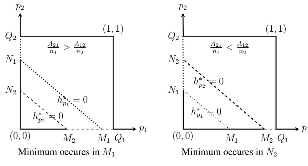
Figure 2. \(\frac{A_{21}}{n_1} \neq \frac{A_{12}}{n_2}\)
(iii) If \(\frac{nA_{12}}{n_2}>\frac{nA_{21}}{n_1}\) and \(\frac{1}{A_{12}}\ln\frac{nA_{12}}{n_2}<1\), then we prove that the minimum of \(h^*\) occurs in \(N_2\). For each point \((p_1,p_2)\) in unit square \([0,1]^2\), there is a unique point \((p_1',p_2)\) on segments \(M_1N_1\) or \(N_1Q_2\) such that \(h^*(p_1',p_2)\leq h^*(p_1,p_2)\). Hence, the minimum of \(h^*\) occurs on \(M_1N_1\cup N_1Q_2\). Also, there is a unique point \((p_1,p_2')\) on segments \(M_2N_2\) or \(M_2Q_1\) such that \(h^*(p_1,p_2')\leq h^*(p_1,p_2)\). Therefore, the minimum of \(h^*\) occurs on \(M_2N_2\cup M_2Q_1\). This two sets of points intersect in one point, \(N_2\), that is, \(h^*(N_2)\leq h^*(p_1,p_2)\) and \(h^*(N_2)=h^*(0,\frac{1}{A_{12}}\ln\frac{nA_{12}}{n_2})=\frac{n_2}{A_{12}}(1+\ln\frac{nA_{12}}{n_2})\).
In each of three cases, if we set \(T = \max\{\frac{nA_{12}}{n_2}, \frac{nA_{21}}{n_1}\}\), then we have :
\[\min_{p_1, p_2} h^*(p_1, p_2) = n(\frac{1 + \ln T}{T}).\]
We now pose a problem.
Problem 3.1. Minimize \(h^*\) if \(\delta_1 = 1\) or \(\delta_2 = 1\).
3.1.2. k is odd
We assume that k is an odd integer and we wish to minimize \(h^*(p_1, p_2)\). For this purpose, we use calculus methodes.
\[\begin{cases} h_{p_1} = n_1 - n_1(A_{11} + 1)e^{-p_1(A_{11} + 1) - p_2A_{12}} - n_2A_{21}e^{-p_1A_{21} - p_2(A_{22} + 1)} \\ h_{p_2} = -n_1A_{12}e^{-p_1(A_{11} + 1) - p_2A_{12}} + n_2 - n_2(A_{22} + 1)e^{-p_1A_{21} - p_2(A_{22} + 1)} \end{cases}\] \[\begin{cases} h_{p_1} = 0 \\ h_{p_2} = 0 \end{cases} \implies \begin{cases} n_1(A_{11} + 1)e^{-p_1(A_{11} + 1) - p_2A_{12}} + n_2A_{21}e^{-p_1A_{21} - p_2(A_{22} + 1)} = n_1 \\ n_1A_{12}e^{-p_1(A_{11} + 1) - p_2A_{12}} + n_2(A_{22} + 1)e^{-p_1A_{21} - p_2(A_{22} + 1)} = n_2 \end{cases}\]
Therefore, we have:
\[\begin{cases} e^{-p_1 A_{21} - p_2 (A_{22} + 1)} = \frac{n_2 (A_{11} + 1) - n_1 A_{12}}{n_2 [A_{12} A_{21} - (A_{11} + 1)(A_{22} + 1)]} \\ e^{-p_1 (A_{11} + 1) - p_2 A_{12}} = \frac{n_1 (A_{22} + 1) - n_2 A_{21}}{n_1 [A_{12} A_{21} - (A_{11} + 1)(A_{22} + 1)]} \end{cases}\]
\(\text{Let } E_1 = \frac{n_2(A_{11}+1) - n_1A_{12}}{n_2[A_{12}A_{21} - (A_{11}+1)(A_{22}+1)]}, \quad E_2 = \frac{n_1(A_{22}+1) - n_2A_{21}}{n_1[A_{12}A_{21} - (A_{11}+1)(A_{22}+1)]}.\) If \(E_1 > 0\) and \(E_2 > 0\), then we have a linear equations system
\[\begin{cases} p_1 A_{21} + p_2 (A_{22} + 1) = -\ln E_1 \\ p_1 (A_{11} + 1) + p_2 A_{12} = -\ln E_2 \end{cases}\]
with a unique answer and we set:
\[\begin{cases} P_1 = \frac{(A_{22} + 1) \ln E_2 - A_{12} \ln E_1}{A_{12}A_{21} - (A_{11} + 1)(A_{22} + 1)} \\ P_2 = \frac{(A_{11} + 1) \ln E_1 - A_{21} \ln E_2}{A_{12}A_{21} - (A_{11} + 1)(A_{22} + 1)} \end{cases}\]
Definition 3.1. A connected bipartite graph G is called 4-perfect if \(E_1>0\), \(E_2>0\) where \(E_1=\frac{n_2(A_{11}+1)-n_1A_{12}}{n_2[A_{12}A_{21}-(A_{11}+1)(A_{22}+1)]}\) and \(E_2=\frac{n_1(A_{22}+1)-n_2A_{21}}{n_1[A_{12}A_{21}-(A_{11}+1)(A_{22}+1)]}.\)
So we get the following.
Corollary 3.1. If G is a 4-perfect graph, \(0 < P_1 < 1\) and \(0 < P_2 < 1\), then
\[\min_{(p_1, p_2) \in (0, 1)^2} h^*(p_1, p_2) = h^*(P_1, P_2) = n_1[E_2 + P_1] + n_2[E_1 + P_2].\]
Note that Corollary 3.1 improves Theorem 2.2 if G is both perfect and 4-perfect. It remains to show that there are perfect graphs that are 4-perfect as well. For this purpose, we consider the graph introduced in Example 3.1.
Example 3.2. Let \(n_1 = n_2 = \frac{n}{2}\), \(\delta_1 = \delta_2 = \delta\), and k = 4m + 1. Thus,
\[E_1 = E_2 = \frac{1}{(2m+1)\delta + 1}\], \(P_1 = P_2 = \frac{\ln[(2m+1)\delta + 1]}{(2m+1)\delta + 1}\)
Since \(E_1, E_2 > 0\), G is 4-perfect. It is also easy to see that G is perfect.
References
- [1] N. Alon and J.H. Spencer, The Probabilistic Method, 2nd ed. John Willy and Sons, INC. New York, USA, (2000).
- [2] I.J. Dejter and O. Serra, Efficient dominating sets in Cayley graphs. Discrete Appl. Math. 129 (2003), 319-328.
- [3] A. Hansberg, D. Meierling and L. Volkmann, Distance domination and distance irredundance in graphs, Electron. J. Combin., 14 (2007), R35.
- [4] T.W. Haynes, S.T. Hedetniemi and P.J. Slater, Fundamentals of domination in graphs, Marcel Dekker, INC. New York, USA, (1998).
- [5] D.A. Mojdeh, A. Sayed-Khalkhali, H. Abdollahzadeh Ahangar and Y. Zhao, Total k-distance domination critical graphs, Transactions on Combinatorics, 5 (3) (2016), 1-9.
- [6] J. Raczek, Distance paired domination numbers of graphs, Discrete Math., 308 (2008), 2473- 2483.
- [7] F. Tian, J-M. Xu, A note on distance domination of graphs, Australas. J. Combin., 43 (2009) 181-190.
- [8] E. Vatandoost, M. Khalili, Domination number of the non-commuting graph of finite groups, Electron. J. Graph Theory Appl. 6 (2) (2018), 228-237.
- [9] D. B. West, Introduction to Graph Theory, 2nd ed. Prentice Hall, USA, (2001).