Abolfazl Poureidi
Faculty of Mathematical Sciences, Shahrood University of Technology, Shahrood, Iran
a.poureidi@shahroodut.ac.ir
A function f : V → {0, 1, 2} is a total Roman dominating function (TRDF) on a graph G = (V, E) if for every vertex v ∈ V with f(v) = 0 there is a vertex u adjacent to v with f(u) = 2 and for every vertex v ∈ V with f(v) > 0 there exists a vertex u ∈ NG(v) with f(u) > 0. The weight of a total Roman dominating function f on G is equal to f(V ) = P v∈V f(v). The minimum weight of a total Roman dominating function on G is called the total Roman domination number of G. In this paper, we give an algorithm to compute the total Roman domination number of a given proper interval graph G = (V, E) in O(|V |) time.
Keywords: Total Roman domination, algorithm, proper interval graph
Mathematics Subject Classification : 05C69
DOI: 10.5614/ejgta.2020.8.2.16
1. Introduction
Let G = (V, E) be a graph with vertex set V and edge set E. Throughout this paper, G = (V, E) is a simple graph with no isolated vertices. The open neighborhood of a vertex v ∈ V is NG(v) = {u ∈ V : uv ∈ E} and the degree of v is deg(v) = |NG(v)|. For any S ⊆ V the induced subgraph G[S] is the graph whose vertex set is S and whose edge set consists of all edges in E that have both endpoints in S. A graph G = (V, E) is an interval graph if there is an one-to-one correspondence between vertices v ∈ V and intervals Iv on the real line. A proper interval graph is an interval graph in which no interval properly contains another. The following is clear.
Received: 16 October 2019, Revised: 4 March 2020, Accepted: 23 September 2020.
Total Roman domination for proper interval graphs | A. Poureidi
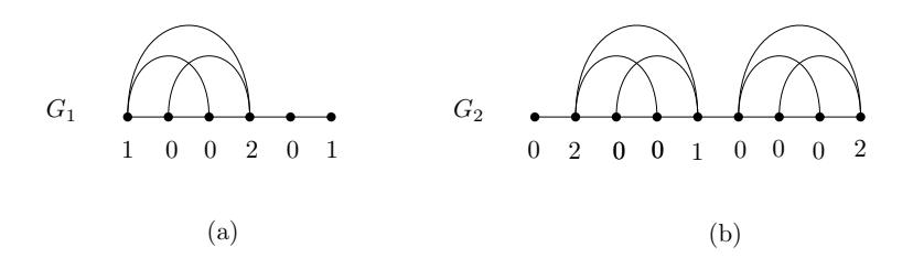
Figure 1. Illustrating (a) an 1-TRDF on G1 and (b) a 2-TRDF on G2.
Proposition 1.1. Let G = (V, E) be a proper interval graph. For any S ⊆ V , the induced subgraph G[S] is a proper interval graph.
For a graph G = (V, E), a Roman dominating function (RDF) of G is a function f : V → {0, 1, 2} such that for every vertex v ∈ V with f(v) = 0 there is a vertex u adjacent to v with f(u) = 2. Stewart [15], and ReVelle and Rosing [14] defined and discussed the concept of Roman domination. Many papers were published on the Roman domination and its several variants, see, for examples, [2, 9, 10].
Liu and Chang [11] introduced a new variant of Roman dominating functions. A RDF f : V → {0, 1, 2} on G is a total Roman dominating function (TRDF) if for every vertex v ∈ V with f(v) > 0 there is a vertex u ∈ NG(v) with f(u) > 0. The weight of a total Roman dominating function f on G is the value f(V ) = P v∈V f(v). The minimum weight of a total Roman dominating function on G is called the total Roman domination number of G, denoted by γtR(G). For further studies on total Roman domination, see, for examples, [1, 3, 4, 5].
Liu and Chang [11] showed that the decision problem related to total Roman domination number is NP-hard even when restricted to bipartite graphs and chordal graphs. Many authors proposed algorithms to compute some variants of domination on proper interval graphs, a well known subclass of chordal graphs, for example, [6, 7, 8, 13]. In this paper we propose a linear algorithm to compute the total Roman domination number of proper interval graphs.
2. Preliminaries
In this section, we introduce some notations that we will use them in our algorithm as follows. Let G = (V, E) be a graph with |V | = n and an ordering (v1, v2, . . . , vn) of vertices of G. Let p ∈ {1, 2}. A function f : V −→ {0, 1, 2} is a p-TRDF on G if f is a RDF with f(vn) = p such that for each u 6= vn with f(u) > 0 there is a vertex x ∈ NG(u) with f(x) > 0. See Figure 1. Let i ∈ {1, 2, . . . , n} and j ∈ {0, 1, 2} , let v0 and vn+1 be vertices not in V and let u, w ∈ V .
- index(vi) = i,
- v + i = vi+1,
- v − i = vi−1,
\[\text{[rumus tidak dapat ditampilkan dengan baik — lihat PDF asli]}\]
• \[MIN(i) = \begin{cases} \min\{j : v_i v_j \in E\}, & \text{if} \quad 1 < i \leq n, \\ 1, & \text{if} \quad i = 1, \end{cases}\]
- MAX(vi) = vMAX(i) ,
- MIN(vi) = vMIN(i) ,
- u ≤ w if j ≤ k, where u = vj and w = vk,
- u < w if j < k, where u = vj and w = vk,
- If u ≤ w, then [u, w] = {z ∈ V : u ≤ z ≤ w},
- If u ≤ w, then G[u, w] = G[{z ∈ V : u ≤ z ≤ w}],
- γ j (G, vi) = min{w(f) : f is a TRDF on G[v1, vi ] with f(vi) = j},
- α p (G, vi) = min{w(f) : f is a p-TRDF on G[v1, vi ]},
- γ(G, vi) = min{w(f) : f is a TRDF on G[v1, vi−1]}.
An ordering (v1, v2, . . . , vn) of vertices of G is a consecutive ordering if vivk ∈ E for some 1 ≤ i < k ≤ n implies both vivj ∈ E and vjvk ∈ E for every i < j < k.
Theorem 2.1 (Looges and Olariu [12]). A graph G is a proper interval graph if and only if G has a consecutive ordering of its vertices.
The following result is clear.
Proposition 2.1. Let G = (V, E) be a connected interval graph of order n with a consecutive ordering (v1, . . . , vn) of vertices of G. If vivj ∈ E for some 1 ≤ i ≤ j ≤ n, then the induced subgraph G[vi , vj ] is the complete graph.
Throughout this paper, for a proper interval graph G of order n, we assume that a consecutive ordering (v1, . . . , vn) of vertices of G is given. If G is a disconnected proper interval graph, then clearly γdR(G) is equal to the sum of the double Roman domination numbers of its components. So, in the following we only consider connected proper interval graphs.
3. Total Roman domination of proper interval graphs
In this section, we propose a linear algorithm (Algorithm 3.1) that computes the total Roman domination number of a given proper interval graph. Let G = (V, E) be a connected proper interval graph with |V | = n ≥ 2 and a consecutive ordering (v1, v2, . . . , vn) of vertices of G.
This algorithm uses a dynamic programming technique for computing the total Roman domination number of G. Algorithm 3.1 first initialize values γ 0 (G, v), γ 1 (G, v), γ 2 (G, v), α 1 (G, v), α 2 (G, v), and γ(G, v) for each v ∈ [v1, MAX(v1)]. By Proposition 2.1, the induced subgraph G[v1, MAX(v1)] is a complete graph. Then, Algorithm 3.1 using values γ 0 (G, v), γ 1 (G, v), γ 2 (G, v), α 1 (G, v), α 2 (G, v), and γ(G, v) for each v ∈ [v1, vi−1] computes values γ 0 (G, vi), γ 1 (G, vi),
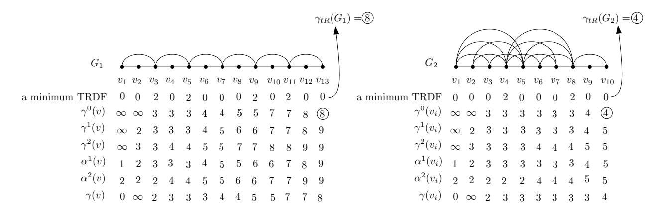
Figure 2. Two examples for illustrating Algorithm 3.1.
\(\gamma^2(G, v_i)\), \(\alpha^1(G, v_i)\), \(\alpha^2(G, v_i)\), and \(\gamma(G, v_i)\) and repeats this process to compute values \(\gamma^0(G, v_n)\), \(\gamma^1(G, v_n)\), \(\gamma^2(G, v_n)\), \(\alpha^1(G, v_n)\), \(\alpha^2(G, v_n)\), and \(\gamma(G, v_n)\). Finally, Algorithm 3.1 returns the value \(\min\{\gamma^0(G, v_n), \gamma^1(G, v_n), \gamma^2(G, v_n)\}\). Examples of Algorithm 3.1 are shown in Figure 2.
To prove Algorithm 3.1 computes the total Roman domination number of proper interval graphs we need the following. Since we have \(x \leftarrow x^+\) (Line 9) in each iteration of the while loop of Algorithm \(TRDN(G, v_1, \ldots, v_n)\), Algorithm \(TRDN(G, v_1, \ldots, v_n)\) terminates. Let \(t_G\) be the number of iterations of the while loop of Algorithm \(TRDN(G, v_1, \ldots, v_n)\).
Lemma 3.1. Let G = (V, E) be a connected proper interval graph with \(|V| = n \ge 2\) and a consecutive ordering \((v_1, v_2, \dots, v_n)\) of vertices of G and let \(i \in \{1, 2, \dots, n\}\), \(j \in \{0, 1, 2\}\) and \(p \in \{1, 2\}\). Then,
- there is a TRDF f on \(G[v_1, v_i]\) with \(f(v_i) = j\) and \(w(f) \le \gamma^j(v_i)\),
- there is a p-TRDF f on \(G[v_1, v_i]\) with \(f(v_i) = p\) and \(w(f) \le \alpha^p(v_i)\), and
- there is a TRDF f on \(G[v_1, v_{i-1}]\) with \(w(f) \leq \gamma(v_i)\).
Proof. Recall that \(t_G\) is the number of iterations of the while loop of Algorithm \(TRDN(G, v_1, \ldots, v_n)\). The proof is by induction on \(t_G\). We first consider the case that the while loop of Algorithm \(TRDN(G, v_1, \ldots, v_n)\) does not hold, that is, \(t_G = 0\). So, we consider Lines 2-7 of Algorithm 3.1. Let \(x = MAX(v_1)\). Since \(t_G = 0\), \(x \ge v_n\). Since always \(MAX(v_1) \le v_n\), \(MAX(v_1) = v_n\), that is, G is the complete graph. In the following we first consider Lines 2-3 and then Lines 5-7 of Algorithm 3.1.
In Lines 2-3 of Algorithm 3.1, we have \(\gamma^0(v_1) = \gamma^1(v_1) = \gamma^2(v_1) = \infty\), \(\alpha^1(v_1) = 1\), \(\alpha^2(v_1) = 2\), \(\gamma(v_1) = 0\), \(\gamma^0(v_2) = \gamma(v_2) = \infty\), \(\gamma^1(v_2) = \alpha^1(v_2) = \alpha^2(v_2) = 2\) and \(\gamma^2(v_2) = 3\). It is not difficult to verify that the lemma holds for both \(v_1\) and \(v_2\).
Here, we consider Lines 5-7 of Algorithm 3.1. Let \(v_i \in [v_3, v_n]\). Recall that G is the complete graph. We have \(\gamma^0(v_3) = \cdots = \gamma^0(x) = 3\) (Line 5). Function \(f = \{(v_1, 2), (v_2, 1), (v_3, 0), \ldots, (v_i, 0)\}\) is a TRDF on \(G[v_1, v_i]\) with \(f(v_i) = 0\) and \(w(f) \leq \gamma^0(v_i) = 3\). We have \(\gamma^1(v_3) = \cdots = \gamma^1(x) = \alpha^1(v_3) = \cdots = \alpha^1(x) = 3\) (Lines 5-6). Function \(\text{[rumus tidak dapat ditampilkan dengan baik — lihat PDF asli]}\)
Algorithm 3.1: TRDN(G, v1, . . . , vn)
Input: A graph G with |V (G)| ≥ 2 and a consecutive ordering (v1, . . . , vn) of vertices of G.
  Output: The total Roman domination number of G.
1 Compute MAX(v1), . . . , MAX(vn), MIN(v1), . . . , MIN(vn);
2 γ
    0
     (v1), γ1
             (v1), γ2
                    (v1) ← ∞; α
                                  1
                                   (v1) ← 1; α
                                               2
                                                (v1) ← 2; γ(v1) ← 0;
3 γ
    0
     (v2), γ(v2) ← ∞; γ
                         1
                          (v2), α1
                                  (v2), α2
                                          (v2) ← 2; γ
                                                      2
                                                       (v2) ← 3; x ← MAX(v1);
4 if x ≥ v3 then
5 γ
        0
         (v3), . . . , γ0
                     (x) ← 3; γ
                                1
                                 (v3), . . . , γ1
                                             (x) ← 3;
6 γ
        2
         (v3), . . . , γ2
                     (x) ← 3; α
                                1
                                 (v3), . . . , α1
                                              (x) ← 3;
7 α
        2
         (v3), . . . , α2
                     (x) ← 2; γ(v3) ← 2; γ(v4), . . . , γ(x) ← 3;
8 while x < vn do
9 x ← x
             +; u ← MIN(x); γ
                               0
                                (x) ← γ
                                         2
                                          (u); γ
                                                2
                                                 (x) ← min{α
                                                                1
                                                                 (u), α2
                                                                        (u)} + 2;
10 α
        2
         (x) ← min{γ(u), α1
                              (u), α2
                                     (u)} + 2; γ(x) ← min{γ
                                                               0
                                                                (x
                                                                   −), γ1
                                                                         (x
                                                                           −), γ2
                                                                                 (x
                                                                                   −)};
11 if u
          + < x then
12 γ
            1
             (x) ← min{α
                           2
                            (MIN(x
                                   −)) + 2, α2
                                               (u) + 1};
13 α
            1
             (x) ← min{γ
                           0
                            (x
                              −), α2
                                    (u)} + 1;
14 else
15 γ
            1
             (x) ← min{α
                           1
                            (u), α2
                                   (u)} + 1;
16 α
            1
             (x) ← min{γ
                           0
                            (u), α1
                                   (u), α2
                                          (u)} + 1;
17 return min{γ
                 0
                  (vn), γ1
                          (vn), γ2
                                  (vn)};
(vi , 1)} is a TRDF on G[v1, vi ] with f(vi) = 1 and w(f) ≤ γ 1 (vi) = 3 and an 1-TRDF on G[v1, vi ] with w(f) ≤ α 1 (vi) = 3. We have γ 2 (v3) = · · · = γ 2 (x) = 3 (Line 6). Function f = {(v1, 1),(v2, 0), . . . ,(vi−1, 0),(vi , 2)} is a TRDF on G[v1, vi ] with f(vi) = 2 and w(f) ≤ γ 2 (vi) = 3. We have α 2 (v3) = · · · = α 2 (x) = 2 (Line 7). Function f = {(v1, 0), . . . ,(vi−1, 0),(vi , 2)} is a 2-TRDF on G[v1, vi ] with w(f) ≤ α 2 (vi) = 2. We have γ(v3) = 2 and γ(v4) = · · · = γ(x) = 3 (Line 7). Function h = {(v1, 1),(v2, 1)} is a TRDF on G[v1, v2] with w(h) ≤ γ(v3) = 2 and f = {(v1, 1),(v2, 2),(v3, 0), . . . ,(vi−1, 0)} is a TRDF on G[v1, vi−1] with w(f) ≤ γ(vi) = 3. So, the base case of the induction holds.
Assume that the claim is true for any connected proper interval graphs H with tH ≤ m, where m ≥ 0. Let us consider a connected proper interval graph G with tG = m + 1. Assume that (v1, v2, . . . , vn) is a consecutive ordering of vertices of G. We have |V (G)| ≥ 3. In the rest of the proof, we consider the last iteration of the while loop of Algorithm TRDN(G, v1, . . . , vn).
Suppose v ∈ V (G). Since the edge MIN(v)v ∈ E(G), by Proposition 2.1, the induced subgraph G[MIN(v), v] is the complete graph. The induced subgraph G[v1, v] is a connected proper interval graph with a consecutive ordering (v1, v2, . . . , v). Consider Algorithm TRDN(G[v1, v], v1, . . . , v). If v < vn, then tG[v1,v] ≤ m. Since x ← x + (Line 9), x = vn ≥ v3 in the last iteration of the while loop of Algorithm TRDN(G, v1, . . . , vn). Assume u = MIN(vn). We have v2 ≤ u ≤ vn−1.
• Instruction γ 0 (vn) ← γ 2 (u) (Line 9 of Algorithm 3.1): The induction hypothesis implies that there is a TRDF h on G[v1, u] with h(u) = 2 and
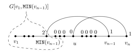
Figure 3. Illustrating a TRDF f on G[v1, vn] with f(vn) = 1 and w(f) ≤ α 2 (MIN(vn−1)) + 2 by using a 2-TRDF on G[v1, MIN(vn−1)] with weight α 2 (MIN(vn−1)); note that some edges are not drawn.
w(h) ≤ γ 2 (u). Consider function f = h ∪ {(u +, 0), . . . ,(vn, 0)}. Function f is a TRDF on G[v1, vn] with f(vn) = 0 and w(f) = w(h) ≤ γ 2 (u) = γ 0 (vn).
• Instruction γ 2 (vn) ← min{α 1 (u), α2 (u)} + 2 (Line 9 of Algorithm 3.1): Let p ∈ {1, 2}. The induction hypothesis implies that there is a p-TRDF hp on G[v1, u] with w(hp) ≤ α p (u). Consider function fp = hp ∪ {(u +, 0), . . . ,(vn−1, 0),(vn, 2)}. Function fp is a TRDF on G[v1, vn] with fp(vn) = 2 and w(f) = w(hp) + 2 ≤ α p (u) + 2. So, there is a TRDF f on G[v1, vn] with f(vn) = 2 and w(f) ≤ min{α 1 (u), α2 (u)} + 2 = γ 2 (vn).
2
+2 = α
α 2
min{α 2
(MIN(vn−1)) + 2, α2
2 (vn).
- Instruction α (vn) ← {γ(u), α1 (u), α2 (u)} + 2 (Line 10 of Algorithm 3.1): The induction hypothesis implies that there is a TRDF h on G[v1, u−] with w(h) ≤ γ(u). Consider function f = h ∪ {(u, 0), . . . ,(vn−1, 0),(vn, 2)}. Function f is a 2-TRDF on G[v1, vn] with w(f) = w(h) + 2 ≤ γ(u) + 2. By the proof of the previous case (Instruction γ 2 (vn) ← min{α 1 (u), α2 (u)} + 2), there is a TRDF g on G[v1, vn] with g(vn) = 2 and w(g) ≤ min{α 1 (u), α2 (u)} + 2. Function g is a 2-
- Instruction γ(vn) ← min{γ 0 (vn−1), γ1 (vn−1), γ2 (vn−1)} (Line 10 of Algorithm 3.1): The induction hypothesis implies that there is a TRDF hj on G[v1, vn−1] with hj (vn−1) = j and w(hj ) ≤ γ j (vn−1), where j ∈ {0, 1, 2}. So, there is a TRDF f on G[v1, vn−1] with w(f) ≤ min{γ 0 (vn−1), γ1 (vn−1), γ2 (vn−1)} = γ(vn).
TRDF on G. Hence, there is a 2-TRDF f on G[v1, vn] with w(f) ≤ min{γ(u), α1
• Instruction γ 1 (vn) ← min{α 2 (MIN(vn−1)) + 2, α2 (u) + 1} (Line 12 of Algorithm 3.1): The induction hypothesis implies that there is a 2-TRDF h on G[v1, u] with w(h) ≤ α 2 (u). Consider function g = h ∪ {(u +, 0), . . . ,(vn−1, 0),(vn, 1)}. Function g is a TRDF on G[v1, vn] with g(vn) = 1 and w(g) = w(h) + 1 ≤ α 2 (u) + 1. The induction hypothesis implies that there is a 2-TRDF h on G[v1, MIN(vn−1)] with w(h) ≤ α 2 (MIN(vn−1)). Consider function g = h∪{(MIN(vn−1) +, 0), . . . ,(vn−2, 0),(vn−1, 1),(vn, 1)}.
See Figure 3. Function g is a TRDF on G[v1, vn] with g(vn) = 1 and w(g) = w(h) + 2 ≤
(MIN(vn−1)) + 2. Hence, there is a TRDF f on G[v1, vn] with f(vn) = 1 and w(f) ≤
1 (vn).
(u) + 1} = γ
(u), α2
(u)}
• Instruction α 1 (vn) ← min{γ 0 (vn−1), α2 (u)} + 1 (Line 13 of Algorithm 3.1):
The induction hypothesis implies that there is a TRDF h on G[v1, vn−1] with h(vn−1) = 0 and w(h) ≤ γ 0 (vn−1). Consider function f = h ∪ {(vn, 1)}. Function f is an 1-TRDF on G[v1, vn] with w(f) = w(h) + 1 ≤ γ 0 (vn−1) + 1 = α 1 (vn).
The induction hypothesis implies that there is a 2-TRDF h on G[v1, u] with w(h) ≤ α 2 (u). Consider function f = h ∪ {(u +, 0), . . . ,(vn−1, 0),(vn, 1)}. Function f is an 1-TRDF on G[v1, vn] with w(f) = w(h) + 1 ≤ α 2 (u) + 1 = α 1 (vn). Hence, there is an 1-TRDF f on G[v1, vn] and w(f) ≤ min{γ 0 (vn−1), α2 (u)} + 1 = α 1 (vn).
• Instruction γ 1 (vn) ← min{α 1 (u), α2 (u)} + 1 (Line 15 of Algorithm 3.1):
The condition of Line 11 does not holds and so u = vn−1. Let p ∈ {1, 2}. The induction hypothesis implies that there is a p-TRDF hp on G[v1, vn−1] with w(hp) ≤ α p (vn−1). Consider function fp = hp ∪ {(vn, 1)}. Function fp is a TRDF on G[v1, vn] with fp(vn) = 1 and w(fp) = w(hp) + 1 ≤ α p (vn−1) + 1. So, there is a TRDF f on G[v1, vn] with f(vn) = 1 and w(f) ≤ min{α 1 (vn−1), α2 (vn−1)} + 1 = γ 1 (vn).
• Instruction α 1 (vn) ← min{γ 0 (u), α1 (u), α2 (u)} + 1 (Line 13 of Algorithm 3.1):
Since the condition of Line 11 does not holds, we have u = vn−1. By the correctness proof of Instruction α 1 (vn) ← {γ 0 (vn−1), α2 (u)}+ 1 (Line 13 of Algorithm 3.1), there is an 1-TRDF g1 on G[v1, vn] with w(g1) ≤ min{γ 0 (vn−1), α2 (vn−1)} + 1.
By the proof of the previous case, there is a TRDF g2 on G[v1, vn] with g2(vn) = 1 and w(g2) ≤ min{α 1 (vn−1), α2 (vn−1)} + 1. Function g2 is an 1-TRDF on G[v1, vn]. Therefore, there is an 1-TRDF f on G[v1, vn] with w(f) ≤ min{γ 0 (vn−1), α1 (vn−1), α2 (vn−1)} + 1 = α 1 (vn).
This completes the proof.
By Lemma 3.1, we have the following result.
Corollary 3.1. Let G = (V, E) be a connected proper interval graph with |V | = n ≥ 2 and a consecutive ordering (v1, v2, . . . , vn) of vertices of G and let γ be the output of Algorithm TRDN(G, v1, . . . , vn). Then, there is a TRDF f on G with w(f) ≤ γ.
Lemma 3.2. Let G = (V, E) be a connected proper interval graph with |V | = n ≥ 2 and a consecutive ordering (v1, v2, . . . , vn) of vertices of G, let i ∈ {1, 2, . . . , n}, j ∈ {0, 1, 2} and p ∈ {1, 2}. Then,
- there is a minimum TRDF f on G[v1, vi ] with f(vi) = j such that γ j (vi) ≤ w(f).
- there is a minimum p-TRDF f on G[v1, vi ] with f(vi) = p such that α p (vi) ≤ w(f), and
- there is a minimum TRDF f on G[v1, vi−1] such that γ(vi) ≤ w(f).
Proof. Recall that tG is the number of iterations of the while loop of Algorithm TRDN(G, v1, . . . , vn). The proof is by induction on tG.
Let G be a graph such that tG = 0. So, Algorithm TRDN(G, v1, . . . , vn) runs only Lines 1-7 of Algorithm 3.1. In Lines 2-3 of Algorithm 3.1, we have
- γ 0 (v1), γ1 (v1), γ2 (v1) ← ∞,
- α 1 (v1) ← 1,
- α 2 (v1) ← 2,
- γ(v1) ← 0,
- γ 0 (v2), γ(v2) ← ∞,
- γ 1 (v2), α1 (v2), α2 (v2) ← 2,
- γ 2 (v2) ← 3
It is not hard to see that γ(G, v1) is equal to 0, α 1 (G, v1) is equal to 1, all α 2 (G, v1), γ 1 (G, v2), α 1 (G, v2) and α 2 (G, v2) are equal to 2, γ 2 (G, v2) is equal to 3 and all γ 0 (G, v1), γ 1 (G, v1), γ 2 (G, v1) γ 0 (G, v2) and γ(G, v2) are undefined.
Let x = MAX(v1) and assume that the condition of Line 4 of Algorithm 3.1 holds, that is, x ≥ v3. Since tG = 0, the condition of Line 8 of Algorithm 3.1 does not hold, that is, x ≥ vn. Hence, x = vn, that is, v1vn ∈ E and so, by Lemma 2.1, G is the complete graph. It is easy to see that the claim holds for each v ∈ [v3, vn]. This proves the base case of the induction.
Assume that the result is true for any connected interval graph H = (V, E) with tH ≥ m, where m ≥ 0. Let G = (V, E) be a connected proper interval graph with tG = m + 1 and a consecutive ordering (v1, v2, . . . , vn) of vertices of G. In the last iteration of the while loop of Algorithm TRDN(G, v1, . . . , vn), we have x = vn. Let v ∈ [v1, vn−1]. The induced subgraph G[v1, v] is a connected interval graph with a consecutive ordering (v1, v2, . . . , v). Consider Algorithm TRDN(G[v1, v], v1, . . . , v). We have tG[v1,v] ≤ m. Let u = MIN(vn). We deduce u ≤ vn−1.
Let f be a minimum TRDF on G with f(vn) = 0, that is, w(f) = γ 0 (G, vn). Since f(vn) = 0, there is a vertex v ∈ [u, vn−1] with f(v) = 2. Since f is a TRDF, there is a vertex v 0 ∈ NG[v1,vn](v) with f(v 0 ) > 0. Since NG[v1,vn](v) ⊆ NG[v1,vn](u), uv0 ∈ E. Assume u 6= v. If we replace f(u) and f(v) by 2 and 0, respectively, then the resulting function is a TRDF on G with weight less than or equal to w(f). Hence, we may assume f(u) = 2. Since NG[v1,vn](v) ⊆ NG[v1,vn](u) for any v ∈ [u, vn], if f(v) = a > 0, then we can replace f(v) and f(MIN(u)), respectively, by 0 and a + b to obtain a new TRDF on G with weight less than or equal to w(f), where f(MIN(u)) = b and the addition in modulo 3. So, we may assume f(v) = 0 for any v ∈ [u +, vn]. Let f 0 be the restriction of f to G[v1, u]. Function f 0 is a TRDF on G[v1, u] with f 0 (u) = 2, that is, γ 2 (G, u) ≤ w(f 0 ). The induction hypothesis implies that there is a minimum TRDF g on G[v1, u] with g(u) = 2 such that γ 2 (u) ≤ w(g). We have w(g) = γ 2 (G, u). Hence, γ 2 (u) ≤ w(g) = γ 2 (G, u) ≤ w(f 0 ) = w(f). In the last iteration of the while loop of Algorithm TRDN(G, v1, . . . , vn) (Line 9), we have γ 0 (vn) ← γ 2 (u). Therefore, γ 0 (vn) ≤ w(f).
Let f be a minimum TRDF on G with f(vn) = 1, that is, w(f) = γ 1 (G, vn). Since f is a TRDF on G and f(vn) = 1, there is a vertex v ∈ [u, vn−1] with f(v) > 0. Since NG[v1,vn](v) ⊆ NG[v1,vn](u), we can replace f(v) and f(u), respectively, by 0 and a + b to obtain a new TRDF on G with weight less than or equal to w(f), where f(v) = a, f(u) = b and the addition in modulo 3. So, we may assume that f(u) > 0 and f(v) = 0 for any v ∈ [u +, vn−1]. We distinguish two cases depending on (i) u < vn−1 or (ii) u = vn−1.
(i) Let u < vn−1.
Since u < vn−1, the condition of Line 11 of Algorithm TRDN(G, v1, . . . , vn) holds in the last iteration of the while loop. We know f(u) ∈ {1, 2}. In the following we consider these cases.
• Let f(u) = 2.
Let f 0 be the restriction of f to G[v1, u]. Since f(v) = 0 for any v ∈ [u +, vn−1], function f 0 is a 2-TRDF on G[v1, u], that is, α 2 (G, u) ≤ w(f 0 ). The induction hypothesis implies that there is a minimum 2-TRDF g on G[v1, u] such that α 2 (u) ≤ w(g). We have w(g) = α 2 (G, u). Hence, α 2 (u) ≤ w(g) = α 2 (G, u) ≤ w(f 0 ) = w(f) − 1, that is, α 2 (u) ≤ w(f) − 1.
• Let f(u) = 1.
Since f(vn−1) = 0, there is a vertex v ∈ [MIN(vn−1), vn−2] with f(v) = 2. Recall f(x) = 0 for any x ∈ [u +, vn−1] and f(u) = 1. So, v ∈ [MIN(vn−1), u−]. Since f(vn) = f(u) = 1, we may assume f(MIN(vn−1)) = 2 and f(v) = 0 for any v ∈ [MIN(vn−1) +, u−]. Let f 0 be the restriction of f to G[v1, MIN(vn−1)]. Function f 0 is a 2-TRDF on G[v1, MIN(vn−1)], that is, α 2 (G, MIN(vn−1)) ≤ w(f 0 ). The induction hypothesis implies that there is a minimum 2-TRDF g on G[v1, MIN(vn−1)] such that α 2 (MIN(vn−1)) ≤ w(g). We have w(g) = α 2 (G, MIN(vn−1)). Hence, α 2 (MIN(vn−1)) ≤ w(g) = α 2 (G, MIN(vn−1)) ≤ w(f 0 ) = w(f) − 2, that is, α 2 (MIN(vn−1)) ≤ w(f) − 2.
Since u < vn−1, in the last iteration of the while loop of Algorithm TRDN(G, v1, . . . , vn) (Line 12), we have γ 1 (vn) ← min{α 2 (MIN(vn−1)) + 2, α2 (u) + 1}. This, together with α 2 (u) ≤ w(f) − 1 and α 2 (MIN(vn−1)) ≤ w(f) − 2, implies that γ 1 (vn) ≤ w(f).
(ii) Let u = vn−1.
Since u = vn−1, f(vn−1) = p ∈ {1, 2}. Let f 0 be the restriction of f to G[v1, vn−1]. Function f 0 is a p-TRDF on G[v1, vn−1], that is, α p (G, vn−1) ≤ w(f 0 ). The induction hypothesis implies that there is a minimum p-TRDF g on G[v1, vn−1] such that α p (vn−1) ≤ w(g). We have w(g) = α p (G, vn−1). Hence, α p (vn−1) ≤ w(g) = α p (G, vn−1) ≤ w(f 0 ) = w(f) − 1, that is, α p (vn−1) ≤ w(f) − 1. In the last iteration of the while loop of Algorithm TRDN(G, v1, . . . , vn) (Line 12), we have γ 1 (vn) ← min{α 1 (u), α2 (u)} + 1. Therefore, γ 1 (vn) ≤ w(f).
Let f be a minimum TRDF on G with f(vn) = 2, that is, w(f) = γ 2 (G, vn). Since f is a TRDF on G and f(vn) = 2, there is a vertex v ∈ [u, vn−1] with f(v) > 0. We may assume f(u) = p ∈ {1, 2} and f(v) = 0 for any v ∈ [u +, vn−1]. Let f 0 be the restriction of f to G[v1, u]. Function f 0 is a p-TRDF on G[v1, u], that is, α p (G, u) ≤ w(f 0 ). The induction hypothesis implies that there is a minimum p-TRDF g on G[v1, u] such that α p (u) ≤ w(g). We have w(g) = α p (G, vn−1). Hence, α p (u) ≤ w(g) = α p (G, vn−1) ≤ w(f 0 ) = w(f) − 2, that is, α p (u) ≤ w(f) − 2. In the last iteration of the while loop of Algorithm TRDN(G, v1, . . . , vn) (Line 9), we have γ 2 (vn) ← min{α 1 (u), α2 (u)} + 2. Therefore, γ 2 (vn) ≤ w(f).
Assume j ∈ {0, 1, 2} and let f be a minimum TRDF on G[v1, vn−1], that is, w(f) = γ(G, vn). Clearly, f(vn−1) ∈ {0, 1, 2}, that is, w(f) = min{γ 0 (G, vn−1), γ1 (G, vn−1), γ2 (G, vn−1)}. The induction hypothesis implies γ j (vn−1) ≤ γ j (G, vn−1). Thus, min{γ 0 (vn−1), γ1 (vn−1), γ2 (vn−1)} ≤ min{γ 0 (G, vn−1), γ1 (G, vn−1), γ2 (G, vn−1)}. In the last iteration of the while loop of Algorithm TRDN(G, v1, . . . , vn) (Line 10), we have γ(vn) ← min{γ 0 (vn−1), γ1 (vn−1), γ2 (vn−1)}. So, γ(vn) ≤ w(f).
Let f be a minimum 1-TRDF on G, that is, w(f) = α 1 (G, vn). We distinguish two cases depending on (i) u < vn−1 or (ii) u = vn−1.
(i) Let u < vn−1.
Assume f(v) = a > 0 for some v ∈ [MIN(vn−1) +, vn−1]. Since NG[v1,vn−1](v) ⊆ NG[v1,vn−1] (MIN(vn−1)), we can replace f(MIN(vn−1)) and f(v) by a + b and 0, respectively, to obtain a new 1-TRDF on G with weight less than or equal to w(f), where f(MIN(vn−1)) = b and the addition in module 3. So, we may assume f(v) = 0 for any v ∈ [MIN(vn−1) +, vn−1]. Since f(vn−1) = 0 and f is a 1-TRDF on G, f(MIN(vn−1)) = 2. Since vn−1 < vn, MIN(vn−1) ≤ u. So, either MIN(vn−1) < u or MIN(vn−1) = u. In the following we consider these cases.
• Assume MIN(vn−1) < u. Let f 0 be the restriction of f to G[v1, vn−1]. Function f 0 is a TRDF on G[v1, vn−1] with f 0 (vn−1) = 0, that is, γ 0 (G, vn−1) ≤ w(f 0 ). The induction hypothesis implies that there is a minimum TRDF g on G[v1, vn−1] with g(vn−1) = 0 such that γ 0 (vn−1) ≤ w(g). We have w(g) = γ 0 (G, vn−1). Hence, γ 0 (vn−1) ≤ w(g) = γ 0 (G, vn−1) ≤ w(f 0 ) = w(f) − 1, that is, γ 0 (vn−1) ≤ w(f) − 1. Since u < vn−1 and MIN(vn−1) < u, in the last iteration of the while loop of Algorithm TRDN(G, v1, . . . , vn) (Line 13), we have 1 0 (vn−1), α2 1
(u)} + 1. Therefore, α
• Assume MIN(vn−1) = u. Let f 0 be the restriction of f to G[v1, u]. Since f(vn) = 1, function f 0 is a 2-TRDF on G[v1, u], that is, α 2 (G, u) ≤ w(f 0 ). The induction hypothesis implies that there is a minimum 2-TRDF g on G[v1, u] such that α 2 (u) ≤ w(g). We have w(g) = α 2 (G, u). Hence, α 2 (u) ≤ w(g) = α 2 (G, u) ≤ w(f 0 ) = w(f) − 1, that is, α 2 (u) ≤ w(f) − 1. Since u < vn−1 and MIN(vn−1) = u, in the last iteration of the while loop of Algorithm TRDN(G, v1, . . . , vn) (Line 13), we have α 1 (vn) ← {γ 0 (vn−1), α2 (u)}+ 1. Therefore, α 1 (vn) ≤ w(f).
(vn) ≤ w(f).
(ii) Let u = vn−1.
α
(vn) ← {γ
Let f 0 be the restriction of f to G[v1, vn−1]. Since u = vn−1 and f is a 1-TRDF on G, f(vn−1) ∈ {0, 1, 2}. In the following we consider these cases.
• Let f(vn−1) = 0 Function f 0 is a TRDF on G[v1, vn−1] with f(vn−1) = 0, that is, γ 0 (G, vn−1) ≤ w(f 0 ). The induction hypothesis implies that there is a minimum TRDF g on G[v1, vn−1] with g(vn−1) = 0 such that γ 0 (vn−1) ≤ w(g). We have w(g) = γ 0 (G, vn−1). Hence, γ 0 (vn−1) ≤ w(g) = γ 0 (G, vn−1) ≤ w(f 0 ) = w(f) − 1, that is, γ 0 (vn−1) ≤ w(f) − 1.
• Let f(vn−1) = p ∈ {1, 2}. Since f(vn) = 1, function f 0 is a p-TRDF on G[v1, vn−1], that is, α p (G, vn−1) ≤ w(f 0 ). The induction hypothesis implies that there is a minimum p-TRDF g on G[v1, vn−1] such that α p (vn−1) ≤ w(g). We have w(g) = α p (G, vn−1). Hence, α p (vn−1) ≤ w(g) = α p (G, vn−1) ≤ w(f 0 ) = w(f) − 1, that is, α p (vn−1) ≤ w(f) − 1.
Since u = vn−1, in the last iteration of the while loop of Algorithm TRDN(G, v1, . . . , vn) (Line 16), we have α 1 (vn) ← min{γ 0 (u), α1 (u), α2 (u)}+1. This, together with γ 0 (vn−1) ≤ w(f) − 1 and α p (vn−1) ≤ w(f) − 1, implies that α 1 (vn) ≤ w(f).
Let f be a minimum 2-TRDF on G, that is, w(f) = α 2 (G, vn). If f(v) = a > 0 for some v ∈ [u +, vn−1], then since NG[v1,vn](v) ⊆ NG[v1,vn](u), we can replace f(u) and f(v) by a + b and 0, respectively, to obtain a new 2-TRDF on G with weight less than or equal to w(f), where f(u) = b and the addition in module 3. So, we may assume f(v) = 0 for any v ∈ [u +, vn−1]. Let f 0 and f 00 be the restrictions of f to G[v1, u] and G[v1, u−], respectively. Clearly, f(u) ∈ {0, 1, 2}. In the following we consider these cases.
- Let f(u) = 0. Function f 00 is a TRDF on G[v1, u−], that is, γ(G, u) ≤ w(f 00). The induction hypothesis implies that there is a minimum TRDF g on G[v1, u−] with g(u) = 0 such that γ(u) ≤ w(g). We have w(g) = γ(G, u). Hence, γ(u) ≤ w(g) = γ(G, u) ≤ w(f 00) = w(f) − 2, that is, γ(u) ≤ w(f) − 2.
- Let f(u) = p ∈ {1, 2}. Function f 0 is a p-TRDF on G[v1, u], that is, α p (G, u) ≤ w(f 0 ). The induction hypothesis implies that there is a minimum p-TRDF g on G[v1, u] such that α p (u) ≤ w(g). We have w(g) = α p (G, u). Hence, α p (u) ≤ w(g) = α p (G, u) ≤ w(f 0 ) = w(f) − 2, that is, α p (u) ≤ w(f) − 2.
In the last iteration of the while loop of Algorithm TRDN(G, v1, . . . , vn) (Line 10), we have α 2 (vn) ← min{γ(u), α1 (u), α2 (u)} + 2. This, together with γ(u) ≤ w(f) − 2 and α p (u) ≤ w(f) − 2, implies that α 2 (vn) ≤ w(f). This completes the proof.
By Lemma 3.2, we have the following result.
Corollary 3.2. Let G = (V, E) be a connected proper interval graph with |V | = n ≥ 2 and a consecutive ordering (v1, v2, . . . , vn) of vertices of G and let γ be the output of Algorithm TRDN(G, v1, . . . , vn). Then, there is a minimum TRDF f on G with γ ≤ w(f).
Theorem 3.1. Let G = (V, E) be a connected proper interval graph with |V | = n ≥ 2 and a consecutive ordering (v1, v2, . . . , vn) of vertices of G. Algorithm TRDN(G, v1, . . . , vn) computes the total Roman domination number of G in O(n) time.
Proof. Let γ be the output of Algorithm TRDN(G, v1, . . . , vn). By Corollaries 3.1 and 3.2, we have γ = γtR(G). In the following we consider the time complexity of Algorithm TRDN(G, v1, . . . , vn). By (Algorithm 2 of) [6], we can compute all values MAX(v1), . . . , MAX(vn) in O(n) time. Clearly,
(vn, vn−1, . . . , v2, v1) is a consecutive ordering of vertices of G. Also, we can compute all values MIN(v1), MIN(v2), . . . , MIN(vn) in O(n) time. It suffices by (Algorithm 2 of) [6] to compute all values MAX(vn), MAX(vn−1), . . . , MAX(v2), MAX(v1) for G with consecutive ordering (vn, vn−1, . . . , v2, v1). So, the running time of Line 1 of Algorithm TRDN(G, v1, . . . , vn) is O(n). Since we know MAX(vi) and MIN(vi) for all i ∈ {1, 2, . . . , n}, the running time of Lines 2-7 of Algorithm TRDN(G, v1, . . . , vn) is O(n) and each iteration of Algorithm TRDN(G, v1, . . . , vn) (Lines 9-16) is O(1). So, the running time of Algorithm TRDN(G, v1, . . . , vn) is O(n). This completes the proof.
References
- [1] H. Abdollahzadeh Ahangar, M.A. Henning, V. Samodivkin and I.G. Yero, Total Roman domination in graphs, Appl. Anal. Discrete Math. 10 (2016), 501–517.
- [2] M.H. Akhbari and N. Jafari Rad, Bounds on weak and strong total domination number in graphs, Electron. J. Graph Theory Appl. 4 (2016), 111–118.
- [3] J. Amjadi, S. Nazari-Moghaddam, S.M. Sheikholeslami and L. Volkmann, Total Roman domination number of trees, Australas. J. Combin. 69 (2017), 271–285.
- [4] J. Amjadi, S.M. Sheikholeslami and M. Soroudi, Nordhaus-Gaddum bounds for total Roman domination, J. Comb. Optim. 35 (2018), 126–133.
- [5] J. Amjadi, S.M. Sheikholeslami and M. Soroudi, On the total Roman domination in trees Discuss. Math. Graph Theory 39 (2019), 519–532.
- [6] T. Araki and H. Miyazaki, Secure domination in proper interval graphs, Discrete Appl. Math. 247 (2018), 70–76.
- [7] A. Braga, C.C. de Souza and O. Lee. The eternal dominating set problem for proper interval graphs, Inform. Process. Lett. 115 (2015), 582–587.
- [8] N. Chiarelli, T.R. Hartinger, V.A. Leoni, M.I.L. Pujato and M. Milanic, New algorithms for ˇ weighted k-domination and total k-domination problems in proper interval graphs, Theoret. Comput. Sci. 795 (2019), 128–141.
- [9] N. Jafari Rad, A note on the edge Roman domination in trees, Electron. J. Graph Theory Appl. 5 (2017), 1–6.
- [10] N. Jafari Rad and H. Rahbani, Some progress on the double Roman domination in graphs, Discuss. Math. Graph Theory 39 (2019), 41–53.
- [11] C.-H. Liu and G.J. Chang, Roman domination on strongly chordal graphs, J. Comb. Optim. 26 (2013), 608–619.
- [12] P.J. Looges and S. Olariu, Optimal greedy algorithms for indifference graphs, Comput. Math. Appl. 25 (1993), 15–25.
- [13] B.S. Panda and S. Paul, A linear time algorithm for liar's domination problem in proper interval graphs, Inform. Process. Lett. 113 (2013), 815–822.
- [14] C.S. Revelle and K. E. Rosing, Defendens imperium romanum: a classical problem in military strategy. Amer. Math. Monthly 107 (2000), 585–594.
- [15] I. Stewart, Defend the roman empire!, Sci. Amer. 281 (1999), 136–139.