Electronic Journal of Graph Theory and Applications
Italo J. Dejter
University of Puerto Rico Rio Piedras, PR 00936-8377
italo.dejter@gmail.com
A sequence \(\mathcal S\) of restricted-growth strings unifies the presentation of middle-levels graphs \(M_k\) as follows, for \(0 < k \in \mathbb Z\). Recall \(M_k\) is the subgraph in the Hasse diagram of the Boolean lattice \(2^{[2k+1]}\) induced by the k- and (k+1)-levels. The dihedral group \(D_{4k+2}\) acts on \(M_k\) via translations mod 2k+1 and complemented reversals. The first \(\frac{(2k)!}{k!(k+1)!}\) terms of \(\mathcal S\) stand for the orbits of \(V(M_k)\) under such \(D_{4k+2}\)-action, via the lexical matching colors \(0,1,\ldots,k\) on the k+1 edges at each vertex. So, \(\mathcal S\) is proposed here as a convenient numeral system for the graphs \(M_k\). Color 0 allows to reorder \(\mathcal S\) via an integer sequence that behaves as an idempotent permutation on its first \(\frac{(2k)!}{k!(k+1)!}\) terms, for each \(0 < k \in \mathbb Z\). Related properties hold for the remaining colors \(1,\ldots,k\).
Keywords: numeral system, middle-levels graph, Boolean lattice, Hasse diagram, complemented reversal Mathematics Subject Classification: 05C62, 05C75, 06A05, 05C69, 05C45 DOI: 10.5614/ejgta.2021.9.1.13
1. Introduction
This paper complements previous work [5] on reinterpreting the middle-levels theorem [6, 8] via a numeral system that enumerates all ordered trees. Let \(0 < k \in \mathbb{Z}\) and let n = 2k + 1. The middle-levels graph \(M_k\) [2, 7] is the subgraph of the Hasse diagram [12] of the Boolean lattice [3], denoted \(2^{[n]}\) and induced by its k- and (k + 1)-th levels (i.e. formed by the k- and (k + 1)-subsets of \([n] = \{0, \ldots, 2k\}\)). The dihedral group \(D_{2n}\) acts on \(M_k\) via translations mod n (see Section 4) and complemented reversals (see Section 5).
Received: 1 May 2018, Revised: 30 December 2020, Accepted: 22 January 2021.
Let \(C_k = \frac{(2k)!}{k!(k+1)!}\) be the k-th Catalan number [13] <u>A000108</u>. Let \(\mathcal{S}\) be the sequence [13] <u>A239903</u> of restricted-growth strings or RGS's ([1] page 325). We will show that the first \(C_k\) terms of \(\mathcal{S}\) stand for the orbits of \(V(M_k)\) under the natural \(D_{2n}\)-action on \((V(M_k), E(M_k))\) in two ways: as Stanley's k-RGS's (see below) and as k-germs, proposed in this work.
In Section 6, the mentioned \(D_{2n}\)-action will allow to project \(M_k\) onto a quotient pseudograph \(R_k\) whose vertices stand for the first \(C_k\) terms of \(\mathcal{S}\) via the Kierstead-Trotter lexical-matching [7] color (or lexical color) set \([k+1] = \{0, 1, \ldots, k\}\) on the k+1 edges incident to each vertex (Sections 7, 8 and 11).
In preparation, RGS's are first tailored in Section 2 into numerical (k-1)-strings \(\alpha\) that are our k-germs. These yield n-strings \(F(\alpha)\) (Section 3), each composed by the k+1 lexical colors, as well as by k asterisks *. The \(F(\alpha)\)'s represent the k-edge ordered trees (Proposition 3.1) and are obtained via a nested substring-swapping, here called castling (Theorem 3.2), that sorts them linearly via pruning and regrafting. These trees (encoded as \(F(\alpha)\)) represent the vertices of \(R_k\) via a corresponding uncastling procedure (Section 8).
The mentioned linear sorting arises from an ordered tree \(\mathcal{T}_k\) (Theorem 3.1) with \(|V(\mathcal{T}_k)| = |V(R_k)| = C_k\). This \(\mathcal{T}_k\) controls \(V(R_k)\) and allows to lexically visualize \(V(M_k)\). On the other hand, an all-RGS's binary tree is given in Section 9, representing the vertices (i.e. the ordered trees) of all \(R_k\)'s. This is a unifying pattern for the presentation of all the \(V(M_k)\)'s.
It is known that the k-edge ordered trees (that is, the vertices of \(R_k\)) denoted by R. Stanley in [14] page 221 item (e) as "plane trees with k+1 vertices", are equivalent to k-strings with initial entry 0, that we shall call k-RGS's, tailored from RGS's in a different way ([14] page 224 item (u)) from that of our k-germs. An equivalence of k-germs and k-RGS's is presented in Section 10 via their distinct relation to the k-edge ordered trees.
Our approach yields a stepwise-reversing presentation (i.e., via complemented-reversal adjacency) of the Hamilton cycles of \(M_k\) [8, 9, 10, 11] in P. Gregor, T. Mütze and J. Nummenpalo [6], that allows an explicit view of all Kierstead-Trotter lexical colors in ordered trees \(F(\alpha)\). The 2-factor \(W_{01}^k\) of \(R_k\) determined by the colors 0 and 1 is reanalyzed from this viewpoint in [5], Section 9, and \(W_{01}^k\) is seen in [5], Section 10, to morph into such Hamilton cycles.
Moreover, an integer sequence \(S_0\) is shown to exist such that, for each k > 0, the neighbors of the vertices of \(R_k\) via color-k edges have their RGS's ordered as in S corresponding to an idempotent permutation on the first \(C_k\) terms of \(S_0\). This and related properties hold for lexical colors \(0, 1, \ldots, k\) (Theorem 11.1 and Remark 11.2) reflecting properties of plane trees (i.e., classes of ordered trees under root rotation).
Incidentally, a sufficient condition [4] (to be compared with [12]), that a path in \(R_k\) lifts to a dihedrally invariant Hamilton cycle in \(M_k\), narrows the conjecture on the existence of Hamilton cycles in \(M_k\), solved in [8], to an unsolved unrestricted version; see Remark 11.3.
2. From restricted-growth strings to k-germs
Let \(0 < k \in \mathbb{Z}\). We can express the mentioned sequence S as: \(S = (\beta(0), \dots, \beta(17), \dots) = (0, 1, 10, 11, 12, 100, 101, 110, 111, 112, 120, 121, 122, 123, 1000, 1001, 1010, 1011, \dots)\) (1)
and note that S has the lengths of its contiguous pairs \((\beta(i-1), \beta(i))\) constant unless \(i = C_k\) for \(0 < k \in \mathbb{Z}\), in which case \(\beta(i-1) = \beta(C_k-1) = 12 \cdots k\) and \(\beta(i) = \beta(C_k) = 10^k = 10 \cdots 0\).
To view the continuation of S, each RGS \(\beta = \beta(m)\) is transformed, for every \(k \in \mathbb{Z}\) with \(k \ge \text{length}(\beta)\), into a (k-1)-string \(\alpha = a_{k-1}a_{k-2}\cdots a_2a_1\) by prefixing k- length\((\beta)\) zeros to \(\beta\). As hinted in Section 1, we say that such an \(\alpha\) is a k-germ. In fact, a k-germ \(\alpha\) \((1 < k \in \mathbb{Z})\) is a (k-1)-string \(\alpha = a_{k-1}a_{k-2}\cdots a_2a_1\) such that:
- (1) the leftmost position (called position k-1) of \(\alpha\) contains entry \(a_{k-1} \in \{0,1\}\);
- (2) given 1 < i < k, the entry \(a_{i-1}\) (at position i-1) satisfies \(0 \le a_{i-1} \le a_i + 1\).
Every k-germ \(a_{k-1}a_{k-2}\cdots a_2a_1\) yields the (k+1)-germ \(0a_{k-1}a_{k-2}\cdots a_2a_1\). A non-null RGS is obtained by stripping a k-germ \(\alpha = a_{k-1}a_{k-2}\cdots a_1 \neq 00\cdots 0\) off all the null entries to the left of its leftmost position containing a 1. We denote such an RGS again by \(\alpha\), convene that the null RGS \(\alpha = 0\) is stripped from all null k-germs \(\alpha\) (\(0 < k \in \mathbb{Z}\)), and use notation \(\alpha = \alpha(m)\) (or \(\beta = \beta(m)\), as in (1)) both for a k-germ and for its corresponding RGS.
The k-germs are ordered as follows. Given two k-germs, say \(\alpha = a_{k-1} \cdots a_2 a_1\) and \(\beta =\)\(b_{k-1} \cdots b_2 b_1\), where \(\alpha \neq \beta\), we say that \(\alpha\) precedes \(\beta\), written \(\alpha < \beta\), whenever either:
- (i) \(a_{k-1} < b_{k-1}\) or
- (ii) \(a_i = b_i\), for \(k 1 \le j \le i + 1\), and \(a_i < b_i\), for some \(k 1 > i \ge 1\).
The resulting order on k-germs \(\alpha(m)\), \((m \leq C_k)\), corresponding biunivocally (via the assignment \(m \to \alpha(m)\)) with the natural order on m, yields a listing that we call the natural (k-germ) listing. Note that there are exactly \(C_k\) k-germs \(\alpha = \alpha(m) < 10^k\), \(\forall k > 0\). Subsection 2.1, deals with the determination of these RGS's and k-germs.
2.1. Catalan's triangle
Given \(0 \le \in \mathbb{Z}\), to determine \(\beta(m)\) or \(\alpha(m)\), we use Catalan's triangle \(\triangle\), i.e. a triangular arrangement of integers starting with the following successive rows \(\Delta_i\), for \(i = 0, \dots, 8\):
\begin{array}{cccccccccccccccccccccccccccccccccccc
where reading is linear, as in [13] A009766. The numbers \(\tau_i^j\) in \(\Delta_j\) (0 \(\leq j \in \mathbb{Z}\)), given by \(\tau_i^j = (j+i)!(j-i+1)/(i!(j+1)!)\), are characterized by the following properties:
- 1. \(\tau_0^j = 1\), for every \(j \ge 0\); 2. \(\tau_1^j = j\) and \(\tau_j^j = \tau_{j-1}^j\), for every \(j \ge 1\);
- 3. \(\tau_i^j = \tau_i^{j-1} + \tau_{i-1}^j\), for every \(j \ge 2\) and \(i = 1, \dots, j-2\); 4. \(\sum_{i=0}^j \tau_i^j = \tau_j^{j+1} = \tau_{j+1}^{j+1} = C_j\), for every \(j \ge 1\).
The determination of k-germ \(\beta(m)\) proceeds as follows. Let \(x_0 = m\) and let \(y_0 = \tau_k^{k+1}\) be the largest member of the second diagonal of \(\triangle\) with \(y_0 \le x_0\). Let \(x_1 = x_0 - y_0\). If \(x_1 > 0\), then let \(Y_1 = \{\tau_{k-1}^j\}_{j=k}^{k+b_1}\) be the largest set of successive terms in the (k-1)-column of \(\triangle\) with
\(y_1=\sum Y_1\leq x_1\). Either \(Y_1=\emptyset\), in which case we take \(b_1=-1\), or not, in which case we take \(b_1=|Y_1|-1\). Let \(x_2=x_1-y_1\). If \(x_2>0\), then let \(Y_2=\{\tau_{k-2}^j\}_{j=k}^{k+b_2}\) be the largest set of successive terms in the (k-2)-column of \(\triangle\) with \(y_2=\sum Y_2\leq x_2\). Either \(Y_2=\emptyset\), in which case we take \(b_2=-1\), or not, in which case we take \(b_2=|Y_3|-1\). Iteratively, we arrive at a null \(x_k\). Then \(\alpha(x_0)=a_{k-1}a_{k-2}\cdots a_1\), where \(a_{k-1}=1\), \(a_{k-2}=1+b_1,\ldots\), and \(a_1=1+b_k\).
We note that \(\beta(m)\) is recovered from \(\alpha(m) = \alpha(x_0)\) by removing the zeros to the left of the leftmost 1 in \(\alpha(x_0)\). Given an RGS \(\beta\) or associated k-germ \(\alpha\), the considerations above can easily be played backwards to recover the corresponding integer \(x_0\).
For example, if \(x_0=38\), then \(y_0=\tau_3^4=14\), \(x_1=x_0-y_0=38-14=24\), \(y_1=\tau_2^3+\tau_2^4=5+9=14\), \(x_2=x_1-y_1=24-14=10\), \(y_2=\tau_1^2+\tau_1^3+\tau_1^4=2+3+4=9\), \(x_3=x_2-y_2=10-9=1\), \(y_3=\tau_0^1=1\) and \(x_4=x_3-y_3=1-1=0\), so that \(b_1=1\), \(b_2=2\), and \(b_3=0\), taking to \(a_4=1\), \(a_3=1+b_1=2\), \(a_2=1+b_2=3\) and \(a_1=1+b_3=1\), determining the 5-germ \(\alpha(38)=a_4a_3a_2a_1=1231\). If \(x_0=20\), then \(y_0=\tau_3^4=14\), \(x_1=x_0-y_0=20-14=6\), \(y_1=\tau_2^3=5\), \(x_2=x_1-y_1=1\), \(y_2=0\) is an empty sum (since its possible summand \(\tau_1^2>1=x_2\)), \(x_3=x_2-y_2=1\), \(y_3=\tau_0^1=1\) and \(x_4=x_3-x_3=1-1=0\), determining the 5-germ \(\alpha(20)=a_4a_3a_2a_1=1101\). Moreover, if \(x_0=19\), then \(y_0=\tau_3^4=14\), \(x_1=x_0-y_0=19-14=5\), \(y_1=\tau_2^3=5\), \(x_2=x_1-y_1=5-5=0\), determining the 5-germ \(\beta(19)=a_4a_3a_2a_1=1100\).
3. Nested substring-swaps in n-strings
An ordered (rooted) tree [6] is a tree T with: (a) a node \(v_0\) as its root; (b) an embedding of T into the plane with \(v_0\) on top; (c) the edges between the nodes at distances j and j+1 from \(v_0\) (\(0 \le j < \operatorname{height}(T)\)) having parent nodes at the j-level above their children at the (j+1)-level; (d) the children in (c) ordered from left to right.
Proposition 3.1. Each k-edge ordered tree T is represented biunivocally by an n-string F(T).
Proof. We perform a depth first search (\(\rightarrow\)DFS) on T with its vertices from \(v_0\) downward denoted \(v_i\) (i = 0, 1, ..., k) in a right-to-left breadth-first search (\(\leftarrow\)BFS) way. Such DFS yields the claimed \(F(\alpha)\) by writing successively from left to right:
- (i) the subindex i of each \(v_i\) in the \(\rightarrow\)DFS downward appearance and
- (ii) an asterisk for each edge \(e_i\) with child \(v_i\) in the \(\rightarrow\)DFS upward appearance.
Theorem 3.1. Each k-germ \(\alpha = a_{k-1} \cdots a_1 \neq 0^{k-1}\) with rightmost nonzero entry \(a_i\) (\(1 \leq i = i(\alpha) < k\)) corresponds to a k-germ \(\beta(\alpha) = b_{k-1} \cdots b_1 < \alpha\) having \(b_i = a_i - 1\) and \(a_j = b_j\) for \(j \neq i\). Moreover, k-germs are the vertices of an ordered tree \(\mathcal{T}_k\) rooted at \(0^{k-1}\), each k-germ \(\alpha \neq 0^{k-1}\) having \(\beta(\alpha)\) as its parent so that the edge \(\beta(\alpha)\alpha\) of \(\mathcal{T}_k\) between \(\beta(\alpha)\) and \(\alpha\) admits a label \(i = i(\alpha)\). Furthermore, the existence of \(\mathcal{T}_k\) allows to sort all k-germs linearly.
Proof. The statement, illustrated for k=2,3,4 in the first three columns of Table I, is straightforward. Table I also serves as illustration for the proof of Theorem 3.2, below.
By representing \(\mathcal{T}_k\) with each node \(\beta\) having its children \(\alpha\) enclosed between parentheses following \(\beta\) and separating siblings with commas, we can write:
\[\mathcal{T}_4 = 000(001, 010(011(012)), 100(101, 110(111(121)), 120(121(122(123))))).\]
- Theorem 3.2. To each k-germ α = ak−1 · · · a1 corresponds biunivocally an n-string F(α) = F(T) = f0f1 · · · f2k whose entries are 0, 1, . . . , k (once each) and k asterisks ∗ such that:
- (A) T is a k-edge ordered tree; (B) F(0k−1 ) = 012 · · ·(k − 1)k ∗ · · · ∗;
- (C) if α 6= 0k−1 , then F(α) is obtained from F(β) = F(β(α)) = h0h1 · · · h2k as in Theorem 3.1 via the following Nested String Swapping (Castling) Procedure, where i = i(α):
- 1. let Wi = h0h1 · · · hi−1 = f0f1 · · · fi−1 and Z i = h2k−i+1 · · · h2k−1h2k = f2k−i+1 · · · f2k−1f2k be respectively the initial and terminal substrings of length i = i(α) in F(β);
- 2. let Ω > 0 be the leftmost entry of the substring U = F(β) \ (Wi ∪ Z i ) and consider the concatenation U = X|Y , with Y starting at entry Ω + 1; then, F(β) = Wi |X|Y |Z i ;
- 3. set F(α) = Wi |Y |X|Z i , (the result of swapping the nested substring X|Y , yielding Y |X).
- In particular: (a) the leftmost entry, f0, of each F(α) is 0; (b) k∗ is a substring of F(α);
- (c) each fj ∈ [0, k] with fj+1 ∈ [0, k) satisfies fj < fj+1, where j ∈ [0, 2k);
- (d) each substring fj ∗ · · · ∗ fj 0 of F(α) (j 00 ∈ (j, j0 ) ⊂ [0, 2k) ⇒ fj 00 = ∗) has fj 0 < fj ;
- (e) Wi is an i-substring with no asterisks; (f) Z i is formed exactly by i asterisks.
TABLE I
| m | α | β | F(β) | i | Wi i | | |Z X Y | Wi i | | |Z Y X | F(α) | α |
|---|---|---|---|---|---|---|---|---|
| 0 | 0 | − | − | − | − | − | 012∗∗ | 0 |
| 1 | 1 | 0 | 012∗∗ | 1 | 0 | 1 | 2∗ |∗ | 0 | 2∗ | 1 |∗ | 02∗1∗ | 1 |
| 0 | 00 | − | − | − | − | − | 012 3 ∗ ∗ ∗ | 00 |
| 1 | 01 | 00 | 0123 ∗ ∗∗ | 1 | 0|1|23 ∗ ∗|∗ | 0|23 ∗ ∗|1|∗ | 023 ∗ ∗ 1 ∗ | 01 |
| 2 | 10 | 00 | ∗ ∗∗ 0123 | 2 | 01|2| ∗ | ∗ ∗ 3 | 01|3 ∗ |2| ∗ ∗ | ∗ ∗ ∗ 013 2 | 10 |
| 3 | 11 | 10 | 013 ∗ 2 ∗ ∗ | 1 | 0|13 ∗ |2 ∗ |∗ | 0|2 ∗ |13 ∗ |∗ | 02 ∗ 13 ∗ ∗ | 11 |
| 4 | 12 | 11 | 02 ∗ 13 ∗ ∗ | 1 | 0|2 ∗ 1|3 ∗ |∗ | 0|3 ∗ |2 ∗ 3|∗ | 03 ∗ 2 ∗ 1∗ | 12 |
| 0 | 000 | − | − | − | − | − | 01234 ∗ ∗ ∗ ∗ | 000 |
| 1 | 001 | 000 | ∗ ∗ ∗ ∗ 01234 | 1 | 0|1|234 ∗ ∗ ∗ | ∗ | 0|234 ∗ ∗ ∗ |1|∗ | ∗ ∗ ∗ ∗ 0234 1 | 001 |
| 2 | 010 | 000 | 01234 ∗ ∗ ∗ ∗ | 2 | 01|2|34 ∗ ∗| ∗ ∗ | 01|34 ∗ ∗|2| ∗ ∗ | 0134 ∗ ∗ 2 ∗ ∗ | 010 |
| 3 | 011 | 010 | 0134 ∗ ∗2 ∗ ∗ | 1 | 0|134 ∗ ∗|2 ∗ | ∗ | 0|2 ∗ |134 ∗ ∗| ∗ | 02 ∗ 134 ∗ ∗ ∗ | 011 |
| 4 | 012 | 011 | ∗ ∗ ∗∗ 02 134 | 1 | 0|2 ∗ 1|34 ∗ ∗| ∗ | 0|34 ∗ ∗|2 ∗ 1| ∗ | ∗ ∗2 ∗ ∗ 034 1 | 012 |
| 5 | 100 | 000 | 01234 ∗ ∗ ∗ ∗ | 3 | 012|3|4 ∗ | ∗ ∗ ∗ | 012|4 ∗ |3| ∗ ∗ ∗ | 0124 ∗ 3 ∗ ∗ ∗ | 100 |
| 6 | 101 | 100 | 0124 ∗ 3 ∗ ∗∗ | 1 | 0|1|24 ∗ 3 ∗ ∗| ∗ | 0|24 ∗ 3 ∗ ∗|1 | ∗ | 024 ∗ 3 ∗ ∗ 1 ∗ | 101 |
| 7 | 110 | 100 | ∗ ∗ ∗∗ 0124 3 | 2 | 01|24 ∗ |3 ∗ | ∗ ∗ | 01|3 ∗ |24 ∗ | ∗ ∗ | ∗ ∗ ∗ ∗ 013 24 | 110 |
| 8 | 111 | 110 | 013 ∗ 24 ∗ ∗∗ | 1 | 0 |13 ∗ |24 ∗ ∗| ∗ | 0|24 ∗ ∗| 13 ∗ | ∗ | 024 ∗ ∗ 13 ∗ ∗ | 111 |
| 9 | 112 | 111 | 024 ∗ ∗13 ∗ ∗ | 1 | 0 |24 ∗ ∗1|3 ∗ | ∗ | 0|3 ∗ |24 ∗ ∗ 1| ∗ | 03 ∗ 24 ∗ ∗ 1 ∗ | 112 |
| 10 | 120 | 110 | ∗ ∗ ∗∗ 013 24 | 2 | 01|3 ∗ 2|4 ∗ | ∗ ∗ | 01|4 ∗ |3 ∗ 2| ∗ ∗ | ∗ ∗ ∗ ∗ 014 3 2 | 120 |
| 11 | 121 | 120 | 014 ∗ 3 ∗ 2∗∗ | 1 | 0|14 ∗ 3 ∗ |2 ∗ |∗ | 0|2 ∗ |14 ∗ 3 ∗ |∗ | 02 ∗ 14 ∗ 3 ∗ ∗ | 121 |
| 12 | 122 | 121 | 02 ∗ 14 ∗ 3∗∗ | 1 | 0|2 ∗ 34 ∗ |3 ∗ |∗ | 0|3 ∗ |2 ∗ 14 ∗ |∗ | 03 ∗ 2 ∗ 14 ∗ ∗ | 122 |
| 13 | 123 | 122 | ∗ ∗ 14∗∗ 03 2 | 1 | 0|3 ∗ ∗ 1|4 ∗ |∗ 2 | 0|4 ∗ |3 ∗ ∗ 1|∗ 2 | ∗ ∗ ∗ 1∗ 04 3 2 | 123 |
Proof. Let α = ak−1 · · · a1 6= 0k−1 be a k-germ. In the sequence of (nested substring-swap) applications of steps 1-3 along the path from root 0 k−1 to α in Tk, unit augmentation of ai for
larger values of i (0 < i < k) must occur earlier, and then in strictly descending order of the entries i of the intermediate k-germs. As a result, the length of the inner substring X|Y is kept non-decreasing after each application. This is illustrated in Table I, where the order of presentation of X and Y is reversed in successively decreasing steps. In the process, items (a)-(e) are seen to be fulfilled.
The three successive subtables in Table I have Ck rows each, where C2 = 2, C3 = 5 and C4 = 14; in the subtables, the k-germs α are shown both on the second and last columns via natural enumeration in the first column; the images F(α) of those α are shown on the penultimate column; the remaining columns in the table are filled, from the second row on, as follows: (i) β = β(α), arising in Theorem 3.1; (ii) F(β), taken from the penultimate column in the previous row; (iii) the length i of Wi and Z i (1 ≤ i ≤ k − 1); (iv) the decomposition Wi |Y |X|Z i of F(β); (v) the nested swapping Wi |X|Y |Z i of Wi |Y |X|Z i , re-concatenated in the following, penultimate, column as F(α), with α = F −1 (F(α)) in the last column.
In the context of the results above, let T = Tα, so F(Tα) = F(α). For each k-germ α 6= 0k−1 , Theorem 3.2 carries a tree-surgery transformation from Tβ onto Tα by pruning-and-regrafting of an adequate subtree of Tβ via the vertices vi and the edges ei , with parent vertices reattached in a substring swapping way. Proposition 3.1 was used in Sections 9-10 [5] in giving a stepwisereversing view of Hamilton cycles [6] in the Mk's.
| m | α | θ(α) | ˆθ(α) | ℵˆ(θ(α)) = ˆθ(α)) ℵ( | ℵ(θ(α)) |
|---|---|---|---|---|---|
| 0 | 0 | 00011 | 0001021∗1∗ | 0∗0∗121110 | 00111 |
| 1 | 1 | 00101 | 00021∗011∗ | 0∗110∗1210 | 01011 |
| 0 | 00 | 0000111 | 000102031∗1∗1∗ | 0∗0∗0∗13121110 | 0001111 |
| 1 | 01 | 0001101 | 0002031∗1∗011∗ | 0∗110∗0∗131210 | 0100111 |
| 2 | 10 | 0001011 | 0001032∗011∗1∗ | 0∗0∗120∗131110 | 0010111 |
| 3 | 11 | 0010011 | 00021∗01031∗1∗ | 0∗0∗13110∗1210 | 0011011 |
| 4 | 12 | 0010101 | 00031∗021∗011∗ | 0∗110∗120∗1310 | 0101011 |
TABLE II
Each F(α) corresponds to a binary n-string θ(α) of weight k obtained by replacing each number in [k + 1] by 0 and each asterisk ∗ by 1. By attaching the entries of F(α) as subscripts to the corresponding entries of θ(α), a subscripted binary n-string ˆθ(α) is obtained, as shown for k = 2, 3 in the fourth column of Table II. Let ℵ(θ(α)) be given by the complemented reversal of θ(α), that is:
if \[\theta(\alpha) = a_0 a_1 \cdots a_{2k}\], then \(\aleph(\theta(\alpha)) = \bar{a}_{2k} \cdots \bar{a}_1 \bar{a}_0\), (2)
where ¯0 = 1 and ¯1 = 0. A subscripted version ℵˆ of ℵ is obtained for ˆθ(α), as shown in the fifth column of Table II, with the subscripts of ℵˆ reversed with respect to those of ℵ. Each image of a k-germ α under ℵ is an n-string of weight k + 1 and has the 1's indexed with subscripts in [k + 1] and the 0's indexed with asterisk subscript. The subscripts in [k + 1] reappear from Section 7 on as lexical colors for the graphs Mk.
4. Translations mod n in \(M_k\)
The n-cube graph \(H_n\) is the Hasse diagram of the Boolean lattice \(2^{[n]}\) on the set [n]. We will express each vertex v of \(H_n\) in three equivalent ways, namely, as:
- (a) ordered set \(A = \{a_0, a_1, \dots, a_{j-1}\} = a_0 a_1 \cdots a_{j-1} \subseteq [n]\) that v represents, \((0 < j \le n)\);
- (b) characteristic binary n-vector \(B_A = (b_0, b_1, \dots, b_{n-1})\) of ordered set A in (a) above, where \(b_i = 1\) if and only if \(i \in A\), \((i \in [n])\);
- (c) polynomial \(\epsilon_A(x) = b_0 + b_1 x + \cdots + b_{n-1} x^{n-1}\) associated to \(B_A\) in (b) above.
The ordered set A and the vector \(B_A\) in (a) and (b) respectively are written for short as \(a_0a_1 \cdots a_{j-1}\) and \(b_0b_1 \cdots b_{n-1}\). A is said to be the support of \(B_A\).
For each \(j \in [n]\), let \(L_j = \{A \subseteq [n]; |A| = j\}\) be the j-level of \(H_n\). Then, \(M_k\) is the subgraph of \(H_n\) induced by \(L_k \cup L_{k+1}\), for \(1 \le k \in \mathbb{Z}\). By viewing the elements of \(V(M_k) = L_k \cup L_{k+1}\) as polynomials, as in (c) above, a regular (i.e., free and transitive) translation mod n action \(\Upsilon'\) of \(\mathbb{Z}_n\) on \(V(M_k)\) is seen to exist, given by:
\[\Upsilon': \mathbb{Z}_n \times V(M_k) \to V(M_k), \text{ with } \Upsilon'(i, v) = v(x)x^i \pmod{1+x^n},\] (3)
where \(v \in V(M_k)\) and \(i \in \mathbb{Z}_n\). Now, \(\Upsilon'\) yields a quotient graph \(M_k/\pi\) of \(M_k\), where \(\pi\) stands for the equivalence relation on \(V(M_k)\) given by:
\[\epsilon_A(x)\pi\epsilon_{A'}(x) \iff \exists i \in \mathbb{Z} \text{ with } \epsilon_{A'}(x) \equiv x^i\epsilon_A(x) \pmod{1+x^n},\]
with \(A, A' \in V(M_k)\). This is used in the proof of Theorem 6.1. Clearly, \(M_k/\pi\) is the graph whose vertices are the equivalence classes of \(V(M_k)\) under \(\pi\). Notice that \(\pi\) induces a partition of \(E(M_k)\) into equivalence classes that are the edges of \(M_k/\pi\).
5. Complemented reversals in \(M_K\)
Let \((b_0b_1\cdots b_{n-1})\) denote the class of \(b_0b_1\cdots b_{n-1}\in L_i\) in \(L_i/\pi\). Let \(\rho_i:L_i\to L_i/\pi\) be the canonical projection given by \(\rho(b_0b_1\cdots b_{n-1})=(b_0b_1\cdots b_{n-1}),\) for \(i\in\{k,k+1\}.\) The definition of the complemented reversal \(\aleph\) in display (2) is easily extended to a bijection, again denoted \(\aleph\), from \(L_k\) onto \(L_{k+1}\). Let \(\aleph_\pi:L_k/\pi\to L_{k+1}/\pi\) be given by \(\aleph_\pi((b_0b_1\cdots b_{n-1}))=(\bar{b}_{n-1}\cdots \bar{b}_1\bar{b}_0).\) Note \(\aleph_\pi\) is a bijection and the identities \(\rho_{k+1}\aleph=\aleph_\pi\rho_k\) and \(\rho_k\aleph^{-1}=\aleph_\pi^{-1}\rho_{k+1}.\)
The following geometric representations are handy. List vertically the vertex parts \(L_k\) and \(L_{k+1}\) of \(M_k\) (resp. \(L_k/\pi\) and \(L_{k+1}/\pi\) of \(M_k/\pi\)) so as to display a splitting of \(V(M_k) = L_k \cup L_{k+1}\) (resp. \(V(M_k)/\pi = L_k/\pi \cup L_{k+1}/\pi\)) into pairs, each pair contained in a horizontal line, the two composing vertices of such pair equidistant from a vertical line \(\phi\) (resp. \(\phi/\pi\), depicted through \(M_2/\pi\) on the left of Figure 1, Section 6 below). In addition, we impose that each resulting horizontal vertex pair in \(M_k\) (resp. \(M_k/\pi\)) be of the form \((B_A,\aleph(B_A))\) (resp. \(((B_A),(\aleph(B_A))=\aleph_\pi((B_A)))\)), disposed from left to right at both sides of \(\phi\). In this context, a non-horizontal edge of \(M_k/\pi\) is said to be a skew edge.
Theorem 5.1. Each skew edge \(e = (B_A)(B_{A'})\) of \(M_k/\pi\) corresponds to another skew edge \(\aleph_{\pi}((B_A))\aleph_{\pi}^{-1}((B_{A'}))\) obtained from e by reflection on the line \(\phi/\pi\). Moreover:
- (i) the skew edges of \(M_k/\pi\) appear in pairs, with the endpoints of the edges in each pair forming two horizontal pairs of vertices equidistant from \(\phi/\pi\);
- (ii) each horizontal edge of \(M_k/\pi\) has multiplicity equal either to 1 or to 2.
Proof. The skew edges \(B_AB_{A'}\) and \(\aleph^{-1}(B_{A'})\aleph(B_A)\) of \(M_k\) are reflection of each other about \(\phi\). Their endopoints form two horizontal pairs \((B_A, \aleph(B_{A'}))\) and \((\aleph^{-1}(B_A), B_{A'})\) of vertices. Now, \(\rho_k\) and \(\rho_{k+1}\) extend together to a covering graph map \(\rho: M_k \to M_k/\pi\), since the edges accompany the projections correspondingly, exemplified for k=2 as follows:
\aleph((B_A)) = \ \aleph((00011)) = \ \aleph(\{00011,10001,11000,01100,00110\}) = \{00111,01110,11100,11001,10011\} = (00111), \\ \aleph^{-1}((B_A')) = \aleph^{-1}((01011)) = \aleph^{-1}(\{01011,10110,10110,11010,10101\}) = \{00101,10010,01001,10100,01010\} = (00101).
Here, the order of the elements in the image of class (00011) (resp. (01011)) mod \(\pi\) under \(\aleph\) (resp. \(\aleph^{-1}\)) are shown reversed, from right to left (cyclically between braces, continuing on the right once one reaches the leftmost brace). Such reversal holds for every k > 2:
\begin{split} &\aleph((B_A)) = & \;\; \aleph((b_0 \cdots b_{2k})) = \;\; \aleph(\{b_0 \cdots b_{2k}, b_{2k} ... b_{2k-1}, ..., b_1 \cdots b_0\}) = \{\bar{b}_{2k} \cdots \bar{b}_0, \bar{b}_{2k-1} \cdots \bar{b}_{2k}, ..., \bar{b}_1 \cdots \bar{b}_0\} = (\bar{b}_{2k} \cdots \bar{b}_0), \\ & \;\; \aleph^{-1}((B_A')) = \aleph^{-1}((\bar{b}_{2k}' \cdots \bar{b}_0')) = \aleph^{-1}(\{\bar{b}_{2k}' \cdots \bar{b}_0', \bar{b}_{2k-1}' \cdots \bar{b}_{2k}', ..., \bar{b}_1' \cdots \bar{b}_0'\}) = \{b_0' \cdots b_{2k}', b_{2k}' \cdots b_{2k-1}', ..., b_1' \cdots b_0'\} = (b_0' \cdots b_{2k}', b_0') = (b_0' \cdots b_{2k}', b_0') = (b_0' \cdots b_{2k}', b_0') = (b_0' \cdots b_{2k}', b_0') = (b_0' \cdots b_0') = (b_0' \cdots b_0') = (b_0' \cdots b_0') = (b_0' \cdots b_0') = (b_0' \cdots b_0') = (b_0' \cdots b_0') = (b_0' \cdots b_0') = (b_0' \cdots b_0') = (b_0' \cdots b_0') = (b_0' \cdots b_0') = (b_0' \cdots b_0') = (b_0' \cdots b_0') = (b_0' \cdots b_0') = (b_0' \cdots b_0') = (b_0' \cdots b_0') = (b_0' \cdots b_0') = (b_0' \cdots b_0') = (b_0' \cdots b_0') = (b_0' \cdots b_0') = (b_0' \cdots b_0') = (b_0' \cdots b_0') = (b_0' \cdots b_0') = (b_0' \cdots b_0') = (b_0' \cdots b_0') = (b_0' \cdots b_0') = (b_0' \cdots b_0') = (b_0' \cdots b_0') = (b_0' \cdots b_0') = (b_0' \cdots b_0') = (b_0' \cdots b_0') = (b_0' \cdots b_0') = (b_0' \cdots b_0') = (b_0' \cdots b_0') = (b_0' \cdots b_0') = (b_0' \cdots b_0') = (b_0' \cdots b_0') = (b_0' \cdots b_0') = (b_0' \cdots b_0') = (b_0' \cdots b_0') = (b_0' \cdots b_0') = (b_0' \cdots b_0') = (b_0' \cdots b_0') = (b_0' \cdots b_0') = (b_0' \cdots b_0') = (b_0' \cdots b_0') = (b_0' \cdots b_0') = (b_0' \cdots b_0') = (b_0' \cdots b_0') = (b_0' \cdots b_0') = (b_0' \cdots b_0') = (b_0' \cdots b_0') = (b_0' \cdots b_0') = (b_0' \cdots b_0') = (b_0' \cdots b_0') = (b_0' \cdots b_0') = (b_0' \cdots b_0') = (b_0' \cdots b_0') = (b_0' \cdots b_0') = (b_0' \cdots b_0') = (b_0' \cdots b_0') = (b_0' \cdots b_0') = (b_0' \cdots b_0') = (b_0' \cdots b_0') = (b_0' \cdots b_0') = (b_0' \cdots b_0') = (b_0' \cdots b_0') = (b_0' \cdots b_0') = (b_0' \cdots b_0') = (b_0' \cdots b_0') = (b_0' \cdots b_0') = (b_0' \cdots b_0') = (b_0' \cdots b_0') = (b_0' \cdots b_0') = (b_0' \cdots b_0') = (b_0' \cdots b_0') = (b_0' \cdots b_0') = (b_0' \cdots b_0') = (b_0' \cdots b_0') = (b_0' \cdots b_0') = (b_0' \cdots b_0') = (b_0' \cdots b_0') = (b_0' \cdots b_0') = (b_0' \cdots b_0') = (b_0' \cdots b_0') = (b_0' \cdots b_0') = (b_0' \cdots b_0') = (b_0' \cdots b_0') = (b_0' \cdots b_0') = (b_0' \cdots b_0') = (b_0' \cdots b_0') = (b_0' \cdots b_0') = (b_0' \cdots b_0') = (b_0' \cdots b_0') = (b_0' \cdots b_0') = (b_0' \cdots b_0') = (b_0' \cdots b_0') = (b_0' \cdots b_0') = (
where \((b_0 \cdots b_{2k}) \in L_k/\pi\) and \((b'_0 \cdots b'_{2k}) \in L_{k+1}/\pi\). This establishes (i).
Every horizontal edge \(v\aleph_\pi(v)\) of \(M_k/\pi\) has \(v\in L_k/\pi\) represented by \(\bar{b}_k\cdots\bar{b}_10b_1\cdots b_k\) in \(L_k\), (so \(v=(\bar{b}_k\cdots\bar{b}_10b_1\cdots b_k)\)). There are \(2^k\) such vertices in \(L_k\) and at most \(2^k\) corresponding vertices in \(L_k/\pi\). For example, \((0^{k+1}1^k)\) and \((0(01)^k)\) are endpoints in \(L_k/\pi\) of two horizontal edges of \(M_k/\pi\), each. To prove that this implies (ii), we have to see that there cannot be more than two representatives \(\bar{b}_k\cdots\bar{b}_1b_0b_1\cdots b_k\) and \(\bar{c}_k\cdots\bar{c}_1c_0c_1\cdots c_k\) of a vertex \(v\in L_k/\pi\), with \(b_0=0=c_0\). Such a v is expressible as \(v=(d_0\cdots b_0d_{i+1}\cdots d_{j-1}c_0\cdots d_{2k})\), with \(b_0=d_i\), \(c_0=d_j\) and \(0< j-i\leq k\). Let the substring \(\sigma=d_{i+1}\cdots d_{j-1}\) be said (j-i)-feasible. Let us see that every (j-i)-feasible substring \(\sigma\) forces in \(L_k/\pi\) only vertices \(\omega\) leading to two different (parallel) horizontal edges in \(M_k/\pi\) incident to v. In fact, periodic continuation mod v of v of v both to the right of v with minimal cyclic substring v only vertices v leading to two different (parallel) for v only with minimal cyclic substring v only vertices v leading to two different (parallel) horizontal edges in v with minimal cyclic substring v only vertices v leading to two different (parallel) horizontal edges in v with minimal cyclic substring v only vertices v leading to two different energy v only vertices v leading to two different energy v both to the right of v only vertices v leading to two different energy v only vertices v leading to two different energy v only vertices v leading to two different energy v only vertices v leading to two different energy v only vertices v leading to two different energy v only vertices v leading v only vertices v leading v only vertices v leading v only v only vertices v leading v only v only v only v only v only v only v only v only v only v only v only v only v only v only v only v only v only v only v only v only v o
(\sigma,\omega) = (\emptyset,(\text{oo1})), (0,(\text{o0o11})), (1,(\text{o1o})), (0^2,(\text{o00o111})), (01,(\text{o01o011})), (1^2,\text{o11o0})), (0^3,\text{o000o1111}), (010,(\text{o010o101101})), (01^2,(\text{o011o})), (101,(\text{o101o})), (1^3,(\text{o111o00})),
with 'o' replacing \(b_0=0\) and \(c_0=0\), and where \(k=\lfloor\frac{n}{2}\rfloor\) has successive values k=1,2,1,3,3,2,4,5,2,3. If \(\sigma\) is a feasible substring and \(\bar{\sigma}=\aleph(\sigma)\), then the possible symmetric substrings \(P_{\phi}\sigma P_r\) about \(o\sigma o=0\sigma 0\) in a vertex v of \(L_k/\pi\) are in order of ascending length:
\begin{array}{c} 0\sigma0,\\ \bar{\sigma}0\sigma0\bar{\sigma},\\ 1\bar{\sigma}0\sigma0\bar{\sigma}1,\\ \sigma1\bar{\sigma}0\sigma0\bar{\sigma}1,\\ \sigma1\bar{\sigma}0\sigma0\bar{\sigma}1\sigma,\\ 0\sigma1\bar{\sigma}0\sigma0\bar{\sigma}1\sigma0,\\ \bar{\sigma}0\sigma1\bar{\sigma}0\sigma0\bar{\sigma}1\sigma0,\\ \bar{\sigma}0\sigma1\bar{\sigma}0\sigma0\bar{\sigma}1\sigma0\bar{\sigma}1,\\ 1\bar{\sigma}0\sigma1\bar{\sigma}0\sigma0\bar{\sigma}1\sigma0\bar{\sigma}1,\\ \end{array}
where we use again '0' instead of 'o' for the entries immediately preceding and following the shown central copy of σ. The lateral periods of Pr and Pφ determine each one horizontal edge at v in Mk/π up to returning to b0 or c0, so no entry e0 = 0 of (d0 · · · d2k) other than b0 or c0 happens such that (d0 · · · d2k) has a third representative e¯k · · · e¯10e1 · · · ek (besides ¯bk · · · ¯b10b1 · · · bk and c¯k · · · c¯10c1 · · · ck). Thus, those two horizontal edges are produced solely from the feasible substrings di+1 · · · dj−1 characterized above.
To illustrate Theorem 5.1, let 1 < h < n in Z be such that gcd(h, n) = 1 and let λh : Lk/π → Lk/π be given by λh((a0a1 · · · an)) → (a0aha2h · · · an−2han−h). For each such h ≤ k, there is at least one h-feasible substring σ and a resulting associated vertex v ∈ Lk/π as in the proof of Theorem 5.1. For example, starting at v = (0k+11 k ) ∈ Lk/π and applying λh repeatedly produces a number of such vertices v ∈ Lk/π. If we assume h = 2h 0 with h 0 ∈ Z, then an h-feasible substring σ has the form σ = ¯a1 · · · a¯h0ah0 · · · a1, so there are at least 2 h 0 = 2 h 2 such h-feasible substrings.
6. Dihedral quotient pseudograph Rk of Mk
An involution of a graph G is a graph map ℵ : G → G such that ℵ 2 is the identity. If G has an involution, an ℵ-folding of G is a graph H, possibly with loops, whose vertices v 0 and edges or loops e 0 are respectively of the form v 0 = {v, ℵ(v)} and e 0 = {e, ℵ(e)}, where v ∈ V (G) and e ∈ E(G); e has endvertices v and ℵ(v) if and only if {e, ℵ(e)} is a loop of G.
Note that both maps ℵ : Mk → Mk and ℵπ : Mk/π → Mk/π in Section 5 are involutions. Let hBAi denote each horizontal pair {(BA), ℵπ((BA))} (as in Theorem 5.1) of Mk/π, where |A| = k. An ℵ-folding Rk of Mk/π is obtained whose vertices are the pairs hBAi and having:
- (1) an edge hBAihBA0i per skew-edge pair {(BA)ℵπ((BA0)),(BA0)ℵπ((BA))};
- (2) a loop at hBAi per horizontal edge (BA)ℵπ((BA)); because of Theorem 5.1, there may be up to two loops at each vertex of Rk.
Theorem 6.1. Rk is a quotient pseudograph of Mk under an action Υ : D2n × Mk → Mk.
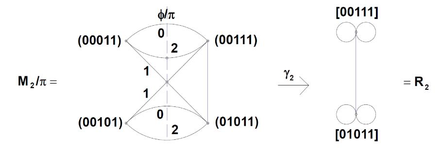
Figure 1. Reflection symmetry of M2/π about a line φ/π and resulting graph map γ2.
Proof. D2n is the semidirect product Zn o% Z2 via the group homomorphism % : Z2 → Aut(Zn), where %(0) is the identity and %(1) is the automorphism i → (n − i), ∀i ∈ Zn. If ∗ : D2n ×
\(D_{2n} \to D_{2n}\) indicates group multiplication and \(i_1, i_2 \in \mathbb{Z}_n\), then \((i_1, 0) * (i_2, j) = (i_1 + i_2, j)\) and \((i_1, 1) * (i_2, j) = (i_1 - i_2, \bar{j})\), for \(j \in \mathbb{Z}_2\). Set \(\Upsilon((i, j), v) = \Upsilon'(i, \aleph^j(v))\), \(\forall i \in \mathbb{Z}_n, \forall j \in \mathbb{Z}_2\), where \(\Upsilon'\) is as in display (3). Then, \(\Upsilon\) is a well-defined \(D_{2n}\)-action on \(M_k\). By writing \((i, j) \cdot v = \Upsilon((i, j), v)\) and \(v = a_0 \cdots a_{2k}\), we have \((i, 0) \cdot v = a_{n-i+1} \cdots a_{2k} a_0 \cdots a_{n-i} = v'\) and \((0, 1) \cdot v' = \bar{a}_{i-1} \cdots \bar{a}_0 \bar{a}_{2k} \cdots \bar{a}_i = (n-i, 1) \cdot v = ((0, 1) * (i, 0)) \cdot v\), leading to the compatibility condition \(((i, j) * (i', j')) \cdot v = (i, j) \cdot ((i', j') \cdot v)\).
Theorem 6.1 yields a graph projection \(\gamma_k: M_k/\pi \to R_k\) for the action \(\Upsilon\), given for k=2 in Figure 1. In fact, \(\gamma_2\) is associated with reflection of \(M_2/\pi\) about the dashed vertical symmetry axis \(\phi/\pi\) so that \(R_2\) (containing two vertices and one edge between them, with each vertex incident to two loops) is given as its image. Both the representations of \(M_2/\pi\) and \(R_2\) in the figure have their edges indicated with colors 0,1,2, as arising inSection 7.
7. Lexical procedure
Let \(P_{k+1}\) be the subgraph of the unit-distance graph of \(\mathbb{R}\) (the real line) induced by the set \([k+1]=\{0,\ldots,k\}\). We draw the grid \(\Gamma=P_{k+1}\square P_{k+1}\) in the plane \(\mathbb{R}^2\) with a diagonal \(\partial\) traced from the lower-left vertex (0,0) to the upper-right vertex (k,k). For each \(v\in L_k/\pi\), there are k+1 n-tuples of the form \(b_0b_1\cdots b_{n-1}=0b_1\cdots b_{n-1}\) that represent v with \(b_0=0\). For each such n-tuple, we construct a 2k-path D in \(\Gamma\) from (0,0) to (k,k) in 2k steps indexed from i=0 to i=2k-1. This leads to a lexical edge-coloring implicit in [7]; see the following statement and Figure 2 (Section 8), containing examples of such a 2k-path D in thick trace.
Theorem 7.1. [7] Each \(v \in L_k/\pi\) has its k+1 incident edges assigned colors \(0, 1, \ldots, k\) by means of the following Lexical Procedure', where \(0 \le i \in \mathbb{Z}\), \(w \in V(\Gamma)\) and D is a path in \(\Gamma\). Initially, let i = 0, w = (0,0) and D contain solely the vertex w. Repeat 2k times the following sequence of steps (1)-(3), and then perform once the final steps (4)-(5):
- (1) If \(b_i = 0\), then set w' := w + (1,0); otherwise, set w' := w + (0,1).
- (2) Reset \(V(D) := v(D) \cup \{w'\}\), \(E(D) := E(D) \cup \{ww'\}\), i := i + 1 and w := w'.
- (3) If \(w \neq (k, k)\), or equivalently, if i < 2k, then go back to step (1).
- (4) Set \(\check{v} \in L_{k+1}/\pi\) to be the vertex of \(M_k/\pi\) adjacent to v and obtained from its representative n-tuple \(b_0b_1\cdots b_{n-1}=0b_1\cdots b_{n-1}\) by replacing the entry \(b_0\) by \(\bar{b}_0=1\) in \(\check{v}\), keeping the entries \(b_i\) of v unchanged in \(\check{v}\) for i>0.
- (5) Set the color of the edge \(v\check{v}\) to be the number c of horizontal (alternatively, vertical) arcs of D above \(\partial\).
Proof. If addition and subtraction in [n] are taken modulo n and we write \([y,x)=\{y,y+1,y+2,\ldots,x-1\}\), for \(x,y\in[n]\), and \(S^c=[n]\setminus S\), for \(S=\{i\in[n]:b_i=1\}\subseteq[n]\), then the cardinalities of the sets \(\{y\in S^c\setminus x:|[y,x)\cap S|<|[y,x)\cap S^c|\}\) yield all the edge colors, where \(x\in S^c\) varies.
The Lexical Procedure of Theorem 7.1 yields a 1-factorization not only for \(M_k/\pi\) but also for \(R_k\) and \(M_k\). This is clarified by the end of Section 8.
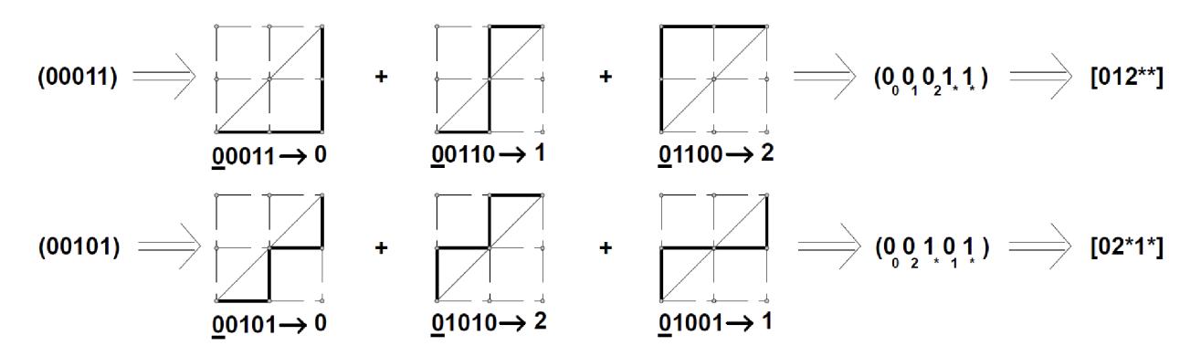
Figure 2. Representing lexical-color assignment for k = 2.
8. Lexical 1-factorization
A notation δ(v) is assigned to each pair {v, ℵπ(v)} ∈ Rk, where v ∈ Lk/π, so that there is a unique k-germ α = α(v) with hF(α)i = δ(v), where the notation h·i appeared for example as in hBAi in Section 6. We exemplify δ(v) for k = 2 in Figure 2, with the Lexical Procedure (indicated by arrows "⇒") departing from v = (00011) (top) and v = (00101) (bottom), passing to sketches of Γ (separated by symbols "+"), one sketch (in which to trace the edges of D ⊂ Γ as in Theorem 7.1) per representative b0b1 · · · bn−1 = 0b1 · · · bn−1 of v shown under the sketch (where b0 = 0 is underscored) and pointing via an arrow "→" to the corresponding color c ∈ [k + 1]. Recall this c is the number of horizontal arcs of D below ∂.
In each of the two cases in Figure 2 (top, bottom), an arrow "⇒" to the right of the sketches points to a modification vˆ of b0b1 · · · bn−1 = 0b1 · · · bn−1 obtained by setting as a subindex of each 0 (resp. 1) its associated color c (resp. an asterisk "∗" ). Further to the right, a third arrow "⇒" points to the n-tuple δ(v) formed by the string of subindexes of entries of vˆ in the order they appear from left to right.
Theorem 8.1. Let α(v 0 ) = ak−1 · · · a1 = 00 · · · 0. Each δ(v) corresponds to a sole k-germ α = α(v) with hF(α)i = δ(v) by means of the following Uncastling Procedure: Given v ∈ Lk/π, let Wi = 01 · · · i be the maximal initial numeric (i.e., colored) substring of δ(v), so that the length of Wi is i + 1 (0 ≤ i ≤ k). If i = k, let α(v) = α(v 0 ); else, set m = 0 and:
- 1. set δ(v m) = hWi |X|Y |Z i i, where Z i is the terminal jm-substring of δ(v m), with jm = i + 1, and let X, Y (in that order) start at contiguous numbers Ω and Ω − 1 ≥ i;
- 2. set δ(v m+1) = hWi |Y |X|Z i i;
- 3. obtain α(v m+1) from α(v m) by increasing its entry ajm by 1;
- 4. if δ(v m+1) = [01 · · · k ∗ · · · ∗], then stop; else, increase m by 1 and go to step 1.
Proof. This is a procedure inverse to that of castling (Section 3), so 1-4 follow.
Theorem 8.1 allows to produce a finite sequence δ(v 0 ), δ(v 1 ), . . . , δ(v m), . . . , δ(v s ) of n-strings with j0 ≥ j1 ≥ · · · ≥ jm · · · ≥ js−1 as in steps 1-4, and k-germs α(v 0 ), α(v 1 ), . . . , α(v m), . . . , α(v s ), taking from α(v 0 ) through the k-germs α(v m), (m = 1, . . . , s − 1), up to α(v) = α(v s ) via unit incrementation of ajm, for 0 ≤ m < s, where each incrementation yields the corresponding
α(v m+1). Recall F is a bijection from the set V (Tk) of k-germs onto V (Rk), both sets being of cardinality Ck. Thus, to deal with V (Rk) it is enough to deal with V (Tk), a fact useful in interpreting Theorem 8.2 below. For example δ(v 0 ) = h04 ∗ 3 ∗ 2 ∗ 1 ∗i = h0|4 ∗ |3 ∗ 2 ∗ 1|∗i = hW0 |X|Y |Z 0 i with m = 0 and α(v 0 ) = 123, continued in Table III with δ(v 1 ) = hW0 |Y |X|Z 0 i, finally arriving to α(v s ) = α(v 6 ) = 000.
TABLE III
| j0=0 | 1 δ(v ) | = | h0|3∗2∗1|4∗|∗i | = | h03∗2∗14∗∗i | = | h0|3∗|2∗14∗|∗i | 1 α(v )=122 | 1 hF(122)i=δ(v ) |
|---|---|---|---|---|---|---|---|---|---|
| j1=0 | 2) δ(v | = | h0|2∗14∗|3∗|∗i | = | h02∗14∗3∗∗i | = | h0|2∗|14∗3∗|∗i | 2)=121 α(v | 2) hF(121)i=δ(v |
| j2=0 | 3 δ(v ) | = | h0|14∗3∗|2∗|∗i | = | h014∗3∗2∗∗i | = | h01|4∗|3∗2|∗∗i | 3 α(v )=120 | 3 hF(120)i=δ(v ) |
| j3=1 | 4) δ(v | = | h01|3∗2|4∗|∗∗i | = | h013∗24∗∗∗i | = | h01|3∗|24∗|∗∗i | 4)=110 α(v | 4) hF(110)i=δ(v |
| j4=1 | 5 δ(v ) | = | h01|24∗|3∗|∗∗i | = | h0124∗3∗∗∗i | = | h012 | 4 ∗|3|∗∗i | 5 α(v )=100 | 5 hF(100)i=δ(v ) |
| j5=2 | 6) δ(v | = | h012|3|4∗|∗∗∗i | = | h01234∗∗∗∗i | 6)=000 α(v | 6) hF(000)i=δ(v |
A pair of skew edges (BA)ℵπ((BA0)) and (BA0)ℵ((BA)) in Mk/π, to be called a skew reflection edge pair (SREP), provides a color notation for any v ∈ Lk+1/π such that in each particular edge class mod π:
- (I) all edges receive a common color in [k + 1] regardless of the endpoint on which the Lexical Procedure (or its modification immediately below) for v ∈ Lk+1/π is applied;
- (II) the two edges in each SREP in Mk/π are assigned a common color in [k + 1]. The modification in step (I) consists in replacing in Figure 2 each v by ℵπ(v) so that on the left we have instead now (00111) (top) and (01011) (bottom) with respective sketch subtitles
00111→0,
01011→0,
           10011→1,
           10101→2,
                       11001→2,
                       01101→1,
resulting in similar sketches when the steps (1)-(5) of the Lexical Procedure are taken with right-toleft reading and processing of the entries on the left side of the subtitles (before the arrows "→"), where the values of each bi must be taken complemented, (i.e., as ¯bi).
Since an SREP in Mk determines a unique edge of Rk (and vice versa), the color received by the SREP can be attributed to , too. Clearly, each vertex of either Mk or Mk/π or Rk defines a bijection from its incident edges onto the color set [k + 1]. The edges obtained via ℵ or ℵπ from these edges have the same corresponding colors.
Theorem 8.2. A 1-factorization of Mk/π by the colors 0, 1, . . . , k is obtained via the Lexical Procedure and can be lifted to a covering 1-factorization of Mk and subsequently collapsed onto a folding 1-factorization of Rk. This validates the notation δ(v), for each v ∈ V (Rk), so that there is a unique k-germ α = α(v) with hF(α)i = δ(v).
Proof. As pointed out in (II) above, each SREP in Mk/π has its edges with a common color in [k+1]. Thus, the [k+1]-coloring of Mk/π induces a well-defined [k+1]-coloring of Rk. This yields the claimed collapsing to a folding 1-factorization of Rk. The lifting to a covering 1-factorization in Mk is immediate. The arguments above determine that the collapsing 1-factorization in Rk induces the claimed k-germs α(v).
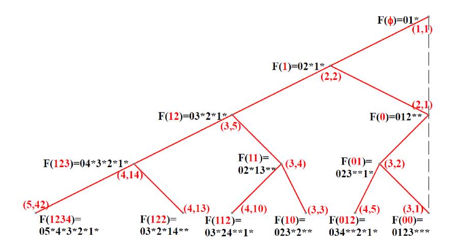
Figure 3. Restriction of T to its first five levels.
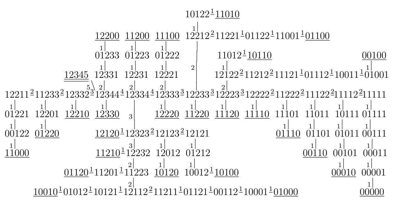
9. All-germs binary tree
The graph R1 has just one vertex 001 with δ(001) = 01∗ (δ as in Section 8) and two loops. Note that the correspondence F in Section 3 has 01∗ as the image of the empty set: F(∅) = 01∗. While Theorem 3.2 allows to sort all k-germs for a fixed k, the following theorem allows to sort all k-germs.
Theorem 9.1. A binary tree T exists with node set ∪ ∞ k=1V (Rk) and such that: (A) its root is 01∗; (B) the left child of a node δ(v) = 0|X in T with ||X|| = 2k (||X|| = length of X) exists and is 0|X + 1|1∗, where X + 1 = (x1 + 1)· · ·(x2k + 1) if X = x1 · · · x2k with color number addition and ∗ + 1 = ∗; (C) unless δ(v) = 01 · · ·(k − 1)k ∗ · · · ∗, it is δ(v) = 0|X|Y |∗, where X and Y are strings starting at some j > 1 and j − 1, respectively, in which case there is a right child of δ(v), namely 0|Y |X|∗, via uncastling. In terms of k-germs, T has each node ak−1ak−2 · · · a2a1 as a parent of a left child bkbk−1 · · · b1 = ak−1ak−2 · · · a2a1(a1 + 1), and as a parent of a right child ρ only if a1 > 0, in which case ρ = ck−1 · · · c2c1 = ak−1 · · · a2(a1 − 1).
Proof. Figure 3 shows the first five levels of T with edges in red and nodes, expressed in terms of red k-germs via F, in otherwise black equalities. To stress the claimed unifying pattern mentioned in Section 1, the figure also assigns to each node a red-colored ordered pair of positive integers (i, j), where j ≤ Ci . The root, given by F(∅) = 01∗, is assigned red (i, j) = (1, 1). The left child of a node assigned red (i, j) is assigned red (k, j0 ) = (i+ 1, j0 ), where j 0 is the order of appearance of the k-germ α corresponding to (k, j0 ) in its presentation via castling as in Table I; α becomes the k-germ corresponding to j 0 in the sequence S (A239903), once the extra zeros to the left of its leftmost nonzero entry are removed. Note j 0 = j 0 (j) arises from the series associated to A076050, deducible from items 1-4 in Subsection 2.1. The right child of a red (i, j) is defined only if j > 1 (strictly to the left of the vertical dotted line); in that case, it is assigned red (i, j − 1).
10. Comparing k-germs and k-RGS's
We show now that the k-germs of Section 2, that were used in all of the above, are equivalent to the sequences of item (u) page 224 [14]. These sequences, that we call k-RGS's in the present context to distinguish them from our k-germs, are indicated in the form \(a_0a_1\cdots a_{k-1}\) satisfying \(a_0=0\) and \(0\leq a_{i+1}\leq a_i+1\). Item (r) page 224 [14] can be used to show that these k-RGS's represent bijectively the k-edge ordered trees, also presented in item (e) page 221 [14]. In fact, let \(b_i=a_i-a_{i+1}+1\) and replace \(a_i\) with one "1" followed by \(b_i\) "-1"s, for \(1\leq i\leq k-1\), where we assume \(a_k=0\), to get a sequence as in item (r), i.e. sequences of k-1 "1"s and k-1 "-1"s such that every partial sum is nonnegative, with "-1" denoted simply as "-".
TABLE IV
| \(01^{\frac{1}{2}}00^{\frac{2}{2}}10^{\frac{1}{2}}11^{\frac{1}{2}}12\) | \[\underline{012}^{\underline{1}}011^{\underline{1}}010^{\underline{2}}\underline{000}^{\underline{3}}100^{\underline{2}}110^{\underline{2}}120^{\underline{1}}121^{\underline{1}}122^{\underline{1}}\underline{123}\] |
|---|---|
| _ | 1 1 1 |
| \(001 \ 101 \ 111^{112}\) | |
| \(10^{1}12^{2}11^{1}01^{1}00\) | \[\underline{100}^{1}012^{1}121^{2}\underline{123}^{3}122^{2}112^{2}111^{1}011^{1}001^{1}\underline{000}\] |
| _ | 1 1 1 |
| \(\underline{120} \ \underline{110} \ 101^{\underline{1}}\underline{010}\) |
For a bijection of the k-edge ordered trees with the sequence in item (r), a depth-first (preorder) search through each k-edge ordered tree is performed: When going "down" an edge (away from the root) records a "1", and when going "up" an edge records a "-1". Thus, the k-germs are in 1-1 correspondence with the RGS's, as claimed. However, each k-germ and its correspondent k-RGS have different expressions, as can be seen by comparing, in the pair of graph subtables in TABLE IV, the tree \(\mathcal{T}_k\) presented with its nodes expressed first as k-germs (top table) and then as k-RGS's (bottom table), for k = 3, 4, where the root is doubly underlined and the leaves are simply underlined, and where k-RGS's are written \(a_1 \cdots a_{k-1}\) instead of \(a_0 a_1 \cdots a_{k-1} = 0 a_1 \cdots a_{k-1}\):
TABLE V
| \(\mid i \mid\) | \(edge label \ subseq of \ell_i\) | \(| first \\ node in \ell_i |\) | \(\begin{array}{c} 2nd \\ node \ in \ \ell_i \end{array}\) | etc. | etc. | etc. | etc. | etc. |
|---|---|---|---|---|---|---|---|---|
| 1 | \(k_1\) | \(01k_3k_2k_1\) | \(01k_3k_2^2\) | _ | _ | _ | _ | _ |
| 2 | \(k_{2}^{2}\) | \(01k_3k_2^2\) | \(01k_3^2k_2\) | \(01k_4k_3^3\) | _ | _ | _ | | — | |
| 3 | \(k_3^{\overline{3}}\) | \(01k_4k_3^{\bar{3}}\) | \(01k_4^2k_3^2\) | \(01k_4^3k_3\) | \(01k_4^4\) | _ | _ | _ | |
| _ | _ | _ | | ||||||
| | j | | \(k_j^j\) | \[01k_{j+1}k_j^j\] | \[01k_{j+1}^2k^{j_1}\] | \[01k_{j+1}^3 k_j^{j_2}\] | \(01k_j^j\) | _ | _ | |
| _ | _ | | |||||||
| \(k_3\) | 3 | \(0123^{k_3}\) | \(012^23^{k_4}\) | \(012^33^{k_5}\) | \(012^{k_2}\) | _ | _ | | |
| \(k_2\) | 2 | \(012^{k_2}\) | \(01^22^{k_3}\) | \(01^32^{k_4}\) | \(01^{k_2}2\) | \(01^{k_1}\) | _ | | |
| \(||k_1||\) | 1 | \(01^{k_1}\) | \(0^21^{k-2}\) | \(0^31^{k_3}\) | \(0^{k_2}1^2\) | \(0^{k_1}1\) | \(0^k\) |
In these representations of \(\mathcal{T}_k\) each edge is given as a short segment with a label \(i=i(\alpha)\) as in Theorem 3.1. Thus, each path from the root to a leaf in \(\mathcal{T}_k\) can be presented by the associated
subsequence of edge labels. From the tables above, we see that the collection of such subsequences for k = 3 is \(\{211, 1\}\), and for k = 4 is \(\{322111, 3211, 31, 211\}\).
Let \(\chi\) be the assignment that to each k-germ \(\alpha\) assigns its associated k-RGS. Expressing k-RGS's as \(a_0a_1\cdots a_{k-1}=0a_1\cdots a_{k-1}\), for example k=3 yields
\[\chi(\underline{00}) = \underline{012}, \ \chi(\underline{01}) = \underline{010}, \ \chi(10) = 011, \ \chi(11) = 001, \ \chi(\underline{12}) = \underline{000}.\]
The lower table above can be taken to represent the trees \(\chi(\mathcal{T}_3)\) and \(\chi(\mathcal{T}_4)\).
The following properties are seen to hold for \(1 < k \in \mathbb{Z}\)
- 1. The root of \(\chi(\mathcal{T}_k)\) and its farthest leaf in \(\chi(\mathcal{T}_i)\) are \(\chi(0^{k-1}) = 012 \cdots (k-1)\) and \(\chi(12 \cdots (k-1)) = 0^k\). Furthermore, the leaves of \(\chi(\mathcal{T}_k)\) are those RGS's \(a_0a_1 \cdots a_{k-1}\) with \(a_{k-1} = 0\).
- 2. Each maximum path \(\ell_i\) of \(\chi(\mathcal{T}_k)\) whose edges have a constant label \(i \in [1, n]\) has initial and terminal nodes of the form \(A_1 = 0a_1a_2\cdots a_n\) and \(A_h = 0(a_2 1)\cdots (a_n 1)(i 1)\).
- 3. By writing \(k_j = k j\), for \(j = 1, \dots, k 1\), the longest path \(\ell\) in \(\chi(\mathcal{T}_k)\) departing from its root has associated edge-label sequence \(k_1 k_2^2 k_3^3 \cdots k_j^j \cdots 2^{k_2} 1^{k_1}\) and is the result of concatenating successively its subpaths \(\ell_i\) as in item 2, described in Table V.
- 4. Each node A of \(\chi(\mathcal{T}_{k+1})\) that is a (k+1)-RGS's having a maximal substring of the form 012...j of length j+1, where j is the sole maximum entry in A, yields a node of \(\chi(\mathcal{T}_k)\) by just removing j from A. All such nodes A of \(\chi(\mathcal{T}_{k+1})\) yield, by these indicated removals, all of \(\chi(\mathcal{T}_k)\). To be used below, let \(\chi''_{k+1}\) be the set of all the nodes A above in this item and let \(\chi'_{k+1} = \chi(\mathcal{T}_{k+1}) \setminus \chi''_{k+1}\).
- 5. Let \((A_1,A_2,\ldots,A_h)\) be a path as in item two in \(\chi'_k\setminus \ell\). To obtain \(A_{i-1}\) from \(A_i=0a_1\cdots a_{k-1}\), for \(i=h,h-1,\ldots,2\), let \(A_i=A'_i|A''_i\) be obtained by the concatenation of the strings \(A'_i=a_0a_1\cdots a_j\) and \(A''_i=a_{j+1}\cdots a_{k-1}\), where \(A'_i=a_0=0\), if \(a_1=0\), and \(A'_i\) is the maximal initial nondecreasing substring of \(A_i\), otherwise, and where \(A''_i=A_i\setminus A'_i\). Then \(A_{i-1}=0|(A''_i\setminus a_{j+1})|(A'_i+1)=0a_{j+2}\cdots a_{k-1}(a_0+1)(a_1+1)\cdots (a_j+1)\).
TABLE VI
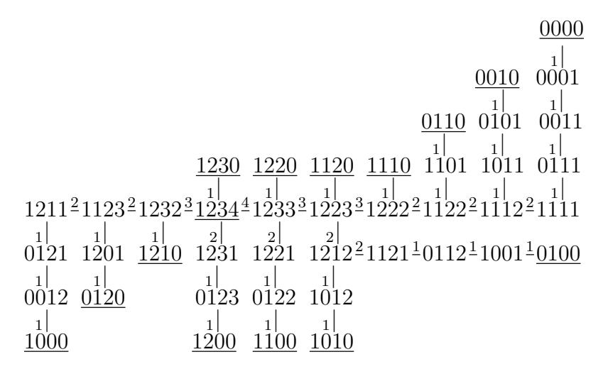
TABLE VII
\[\text{[rumus tidak dapat ditampilkan dengan baik — lihat PDF asli]}\]
Tables VI and VII contain respective representations of \(\chi(\mathcal{T}_5)\) and \(\chi_6''\), the latter one here with a bar over the maximal entry of each RGS node, as in item 4, entry whose removal yields a corresponding node of \(\chi(\mathcal{T}_4)\).
As an additional example here, Table VIII contains a representation of \(\chi'_6\).
By considering the order-number permutations (as in the left column in Table I above) via \(\chi\) we obtain permutations as follows:
\[\text{[rumus tidak dapat ditampilkan dengan baik — lihat PDF asli]}\]
TABLE VIII
11. Colored germ adjacency
TABLE IX
| \(\parallel m \parallel\) | \(\mid \alpha \mid\) | \(F(\alpha)\) | \(F^3(\alpha)\) | \(F^{2}(\alpha)\) | \(F^1(\alpha)\) | \(F^0(\alpha)\) | \(\alpha^3\) | \(\alpha^2\) | \(\alpha^1\) | \(\mid \alpha^0 \mid \mid\) |
|---|---|---|---|---|---|---|---|---|---|---|
| 0 | 0 | 012 * * | _ | 012 * * | 02 * 1* | 12**0 | _ | 0 | 1 | 0 |
| 1 | 1 | 02 * 1* | _ | 1 * 02* | 012 * * | 2*1*0 | _ | 1 | 0 | 1 |
| 0 | 00 | 0123*** | 0123 *** | 013*2** | 023**1* | 123***0 | 00 | 10 | 01 | 00 |
| 1 | 01 | 023**1* | 1*023** | 1*03*2* | 0123 *** | 2*13**0 | 01 | 12 | 00 | 11 |
| ||2| | 10 | 013*2** | 02*20** | 0123*** | 03*2*1* | 13*2**0 | 11 | 00 | 12 | 10 |
| 3 | 11 | 02*13** | 013*2** | 13**02* | 02*13** | 10**2*3 | 10 | 11 | 11 | 01 |
| 4 | 12 | 03*2*1* | 2*1*03* | 1*023** | 013*2** | 3*2*1*0 | 12 | 01 | 10 | 12 |
Given a k-germ \(\alpha\), let \((\alpha)\) represent the dihedral class \(\delta(v) = \langle F(\alpha) \rangle\) with \(v \in L_k/\pi\). Recall \(W_{01}^k\) is the 2-factor given by the union of the 1-factors of colors 0, 1 in \(M_k\) (namely those formed by lifting the edges \(\alpha\alpha^0\), \(\alpha\alpha^1\) of \(R_k\) in the notation below in this section, instead of those of colors k, k-1, as in [6]).
We present each \(c \in V(R_k)\) via the pair \(\delta(v) = \{v, \aleph_{\pi}(v)\} \in R_k\) (\(v \in L_k/\pi\)) of Section 8 and via the k-germ \(\alpha\) for which \(\delta(v) = \langle F(\alpha) \rangle\), and view \(R_k\) as the graph whose vertices are the k-germs \(\alpha\), with adjacency inherited from that of their \(\delta\)-notation via \(F^{-1}\) (i.e. uncastling). So, \(V(R_k)\) is presented as in the natural (k-germ) listing (see Section 2).
To start with, examples of such presentation are shown in Table IX for k=2 and 3, where m, \(\alpha=\alpha(m)\) and \(F(\alpha)\) are shown in the first three columns, for \(0\leq m< C_k\). The neighbors of \(F(\alpha)\) are presented in the central columns of the table as \(F^k(\alpha)\), \(F^{k-1}(\alpha)\), ..., \(F^0(\alpha)\) respectively for the edge colors \(k, k-1, \ldots, 0\), with notation given via the effect of function \(\aleph\). The last columns yield the k-germs \(\alpha^k\), \(\alpha^{k-1}\), ..., \(\alpha^0\) associated via \(F^{-1}\) respectively to the listed neighbors \(F^k(\alpha)\), \(F^{k-1}(\alpha)\), ..., \(F^0(\alpha)\) of \(F(\alpha)\) in \(R_k\).
TABLE X
| \(\mid m \mid\) | \(\alpha\) | \(\alpha^4\) | \(\alpha^3\) | \(\alpha^2\) | \(\alpha^1\) | \(\alpha^0\) | m | \(\alpha\) | \(\alpha^4\) | \(\alpha^3\) | \(\alpha^2\) | \(\alpha^1\) | \(\mid \alpha^0 \mid\) | l | |
|---|---|---|---|---|---|---|---|---|---|---|---|---|---|---|---|
| | _ | | | | | l —— | _ | | | | l —— | | | | ı | ||||||||
| 0 | 000 | 000 | 100 | 010 | 001 | 000 | 7 | 110 | 100 | 111 | 110 | 012 | 010 | l | |
| 1 | 001 | 001 | 101 | 012 | 000 | 011 | 8 | 111 | 111 | 110 | 122 | 011 | 111 | ||
| 2 | 010 | 011 | 121 | 000 | 112 | 110 | 9 | 112 | 101 | 122 | 112 | 010 | 112 | İ | |
| 3 | 011 | 010 | 120 | 011 | 111 | 001 | 10 | 120 | 122 | 011 | 100 | 123 | 120 | ||
| İ | 4 | 012 | 012 | 123 | 001 | 110 | 122 | 11 | 121 | 121 | 010 | 121 | 122 | 101 | İ |
| 5 | 100 | 110 | 000 | 120 | 101 | 100 | 12 | 122 | 120 | 112 | 111 | 121 | 012 | ||
| 6 | 101 | 112 | 001 | 123 | 100 | 121 | 13 | 123 | 123 | 012 | 101 | 120 | 123 | İ | |
| ĺ | |||||||||||||||
| İ | l – I | | | | | | _ | | | | | | | | | İ | |||||||
| 3** | *** | 3** | *2* | **1 | 3** | *** | 3** | *2* | **1 | l |
For k=4 and 5, Tables X and XI have a similar respective natural enumeration adjacency disposition. We can generalize these tables directly to Colored Adjacency Tables denoted CAT(k), for k>1. This way, Theorem 11.1(A) below is obtained as indicated in the aggregated last row upending Tables X and XI citing the only non-asterisk entry, for each of \(i=k,k-2,\ldots,0\), as a number \(j=(k-1),\ldots,1\) that leads to entry equality in both columns \(\alpha=a_{k-1}\cdots a_j\cdots a_1\) and \(\alpha^i=a_{k-1}^i\cdots a_j^i\cdots a_1^i\), that is \(a_j=a_j^i\). Other important properties are contained in the remaining items of Theorem 11.1, including (B), that the columns \(\alpha^0\) in all CAT(k), (k>1), yield an (infinte) integer sequence.
Theorem 11.1. Let: k > 1, \(j(\alpha^k) = k - 1\) and \(j(\alpha^{i-1}) = i\), (i = k - 1, ..., 1). Then: (A) each column \(\alpha^{i-1}\) in CAT(k), for \(i \in [k] \cup \{k+1\}\), preserves the respective \(j(\alpha^{i-1})\)-th entry of \(\alpha\); (B) the columns \(\alpha^k\) of all CAT(k)'s for k > 1 coincide into an RGS sequence and thus into an integer sequence \(S_0\), the first \(C_k\) terms of which form an idempotent permutation for each k; (C) the integer sequence \(S_1\) given by concatenating the m-indexed intervals \([0,2),[2,5),\ldots\), \([C_{k-1},C_k)\), etc. in column \(\alpha^{k-1}\) of the corresponding tables CAT(2), CAT\((3),\ldots\), CAT(k), etc. allows to encode all columns \(\alpha^{k-1}\)'s; (D) for each k > 1, there is an idempotent permutation given in the m-indexed interval \([0,C_k)\) of the column \(\alpha^{k-1}\) of CAT(k); such permutation equals the one given in the interval \([0,C_k)\) of the column \(\alpha^{k-2}\) of CAT(k+1).
Proof. (A) holds as a continuation of the observation made above with respect to the last aggregated row in Tables X and XI. Let \(\alpha\) be a k-germ. Then \(\alpha\) shares with \(\alpha^k\) (e.g. the leftmost column \(\alpha^i\) in Tables VIII to X, for \(0 \le i \le k\)) all the entries to the left of the leftmost entry 1, which yields (B). Note that if k=3 then m=2,3,4 yield for \(\alpha^{k-1}\) the idempotent permutation (2,0)(4,1), illustrating (C). (D) can be proved similarly.
TABLE XI
| \(\mid m \mid\) | \(\alpha\) | \(\alpha^5\) | \(\alpha^4\) | \(\alpha^3\) | \(\alpha^2\) | \(\alpha^1\) | \(\alpha^0\) | | | | |m| | \(\alpha\) | \(\alpha^5\) | \(\alpha^4\) | \(\alpha^3\) | \(\alpha^2\) | \(\alpha^1\) | \(\mid \alpha^0 \mid \mid\) |
|---|---|---|---|---|---|---|---|---|---|---|---|---|---|---|---|---|
| | - | | | | | | | | | || | | | - | | | | | | | | | | | | | |||||
| | 0 | 0000 | 0000 | 1000 | 0100 | 0010 | 0001 | 0000 | 21 | 1110 | 1111 | 1100 | 1221 | 0110 | 1112 | | 1110 || | |
| 1 | 0001 | 0001 | 1001 | 0101 | 0012 | 0000 | 0011 | | 22 | | 1111 | 1110 | 1111 | 1220 | 0122 | 1111 | 0111 | |
| || 2 | 0010 | 0011 | 1011 | 0121 | 0000 | 0112 | 0110 | || | | 23 | 1112 | 1122 | 1101 | 1233 | 0112 | 1110 | | 1222 | |
| | 3 | 0011 | 0010 | 1010 | 0120 | 0011 | 0111 | 0001 | 24 | 1120 | 1011 | 1222 | 1121 | 0100 | 1123 | 1120 | |
| 4 | 0012 | 0012 | 1012 | 0123 | 0001 | 0110 | 0122 | ii i | 25 | 1121 | 1010 | 1221 | 1120 | 0121 | 1122 | 0101 |
| 5 | 0100 | 0110 | 1210 | 0000 | 1120 | 1101 | 1100 | 26 | 1122 | 1112 | 1220 | 1223 | 0111 | 1121 | 1122 | |
| 6 | 0101 | 0112 | 1212 | 0001 | 1123 | 1100 | 1121 | ii i | 27 | 1123 | 1012 | 1233 | 1123 | 0101 | 1120 | | 1223 || |
| 7 | 0110 | 0100 | 1200 | 0111 | 1110 | 0012 | 0010 | 28 | 1200 | 1220 | 0110 | 1000 | 1230 | 1201 | 1200 | |
| 8 | 0111 | 0111 | 1211 | 0110 | 1122 | 0011 | 1111 | ii i | 29 | 1201 | 1223 | 0112 | 1001 | 1234 | 1200 | | 1231 || |
| 9 | 0112 | 0101 | 1201 | 0122 | 1112 | 0010 | 0112 | 30 | 1210 | 1210 | 0100 | 1211 | 1220 | 1012 | 1011 | |
| 10 | 0120 | 0122 | 1232 | 0011 | 1100 | 1223 | 1220 | ii i | 31 | 1211 | 1222 | 0111 | 1210 | 1233 | 1011 | 1221 |
| 11 | 0121 | 0121 | 1231 | 0010 | 1121 | 1222 | 1101 | 32 | 1212 | 1212 | 0101 | 1232 | 1223 | 1010 | | 1212 || | |
| 12 | 0122 | 0120 | 1230 | 0112 | 1111 | 1221 | 0012 | ii i | 33 | 1220 | 1200 | 1122 | 1111 | 1210 | 0123 | 0120 |
| 13 | 0123 | 0123 | 1234 | 0012 | 1101 | 1220 | 1233 | 34 | 1221 | 1221 | 1121 | 1110 | 1232 | 0122 | 1211 | |
| 14 | 1000 | 1100 | 0000 | 1200 | 1010 | 1001 | 1000 | ii i | 35 | 1222 | 1211 | 1120 | 1222 | 1222 | 0121 | | 1112 || |
| 15 | 1001 | 1101 | 0001 | 1201 | 1012 | 1000 | 1011 | 36 | 1223 | 1201 | 1223 | 1122 | 1212 | 0120 | | 1123 || | |
| 16 | 1010 | 1121 | 0011 | 1231 | 1000 | 1212 | 1210 | ii i | 37 | 1230 | 1233 | 0122 | 1011 | 1200 | 1234 | 1230 |
| 17 | 1011 | 1120 | 0010 | 1230 | 1011 | 1211 | 1001 | 38 | 1231 | 1232 | 0121 | 1010 | 1231 | 1233 | 1201 | |
| 18 | 1012 | 1123 | 0012 | 1234 | 1001 | 1210 | 1232 | 39 | 1232 | 1231 | 0120 | 1212 | 1221 | 1232 | 1012 | |
| 19 | 1100 | 1000 | 1110 | 1100 | 0120 | 0101 | 0100 | 40 | 1233 | 1230 | 1123 | 1112 | 1211 | 1231 | 0123 | |
| 20 | 1101 | 1001 | 1112 | 1101 | 0123 | 0100 | 0121 | ii i | 41 | 1234 | 1234 | 0123 | 1012 | 1201 | 1230 | 1234 |
| || -0 | | | | | | | | | | ==00 | | | | | | | | | | -=-00 | | | |||||
| | | _ | | | | | | | | | _ | | | | | | | | | |||||||||
| 4*** | **** | 4*** | *3** | **2* | ***1 | 4*** | **** | 4*** | *3** | **2* | ***1 |
The sequences in Theorem 11.1 (B)-(C) start as follows, with intervals ended in ";":
\[\text{[rumus tidak dapat ditampilkan dengan baik — lihat PDF asli]}\]
Given a k-germ \(\alpha = a_{k-1} \cdots a_1\), we want to express \(\alpha^k, \alpha^{k-1}, \ldots, \alpha^0\) as functions of \(\alpha\). Given a substring \(\alpha' = a_{k-j} \cdots a_{k-i}\) of \(\alpha\) (\(0 < j \le i < k\)), let: (a) the reverse string off \(\alpha'\) be \(\psi(\alpha') = a_{k-i} \cdots a_{k-j}\); (b) the ascent of \(\alpha'\) be (i) its maximal initial ascending substring, if \(a_{k-j} = 0\), and (ii) its maximal initial non-descending substring with at most two equal nonzero terms, if \(a_{k-j} > 0\). Then, the following remarks allow to express the k-germs \(\alpha^p = \beta = b_{k-1} \cdots b_1\) via the colors \(p = k, k-1, \ldots, 0\), independently of \(F^{-1}\) and F.
Remark 11.1. Assume p=k. If \(a_{k-1}=1\), take \(0|\alpha\) instead of \(\alpha=a_{k-1}\cdots a_1\), with k-1 instead of k, removing afterwards from the resulting \(\beta\) the added leftmost 0. Now, let \(\alpha_1=a_{k-1}\cdots a_{k-i_1}\) be the ascent of \(\alpha\). Let \(B_1=i_1-1\), where \(i_1=||\alpha_1||\) is the length of \(\alpha_1\). It can be seen that \(\beta\) has ascent \(\beta_1=b_{k-1}\cdots b_{k-i_1}\) with \(\alpha_1+\psi(\beta_1)=B_1\cdots B_1\). If \(\alpha\neq\alpha_1\), let \(\alpha_2\) be the ascent of \(\alpha\setminus\alpha_1\). Then there is a \(||\alpha_2||\)-germ \(\beta_2\) with \(\alpha_2+\psi(\beta_2)=B_2\cdots B_2\) and \(B_2=||\alpha_1||+||\alpha_2||-2\). Inductively when feasible for j>2, let \(\alpha_j\) be the ascent of \(\alpha\setminus(\alpha_1|\alpha_2|\cdots|\alpha_{j-1})\). Then there is a \(||\alpha_j||\)-germ \(\beta_j\) with \(\alpha_j+\psi(\beta_j)=B_j\cdots B_j\) and \(B_j=||\alpha_{j-1}||+||\alpha_j||-2\). This way, \(\beta=\beta_1|\beta_2|\cdots|\beta_j|\cdots\). Remark 11.2. Assume k>p>0. By Theorem 11.1 (A), if p< k-1, then \(b_{p+1}=a_{p+1}\); in this case, let \(\alpha'=\alpha\setminus\{a_{k-1}\cdots a_q\}\) with q=p+1. If p=k-1, let q=k and let \(\alpha'=\alpha\). In both cases (either p< k-1 or p=k-1) let \(\alpha'_1=a_{q-1}\cdots a_{k-i_1}\) be the ascent of \(\alpha'\). It can be seen that \(\beta'=\beta\setminus\{b_{k-1}\cdots b_q\}\) has ascent \(\beta'_1=b_{k-1}\cdots b_{k-i_1}\) where \(\alpha'_1+\psi(\beta'_1)=B'_1\cdots B'_1\) with \(B'_1=i_1+a_q\). If \(\alpha'\neq\alpha'_1\) then let \(\alpha'_2\) be the ascent of \(\alpha'\setminus\alpha'_1\). Then there is a \(||\alpha'_2||\)-germ \(\beta'_2\) where \(\alpha'_2+\psi(\beta'_2)=B'_2\cdots B'_2\) with \(B'_2=||\alpha'_1||+||\alpha'_2||-2\). Inductively when feasible for j>2, let \(\alpha_j\) be
We process the left-hand side from position q. If p>1, we set \(a_{a_q+2}\cdots a_q+\psi(b_{b_q+2}\cdots b_q)\) to equal a constant string \(B\cdots B\), where \(a_{a_q+2}\cdots a_q\) is an ascent and \(a_{a_q+2}=b_{b_q+2}\). Expressing all those numbers \(a_i,b_i\) as \(a_i^0,b_i^0\), respectively, in order to keep an inductive approach, let \(a_q^1=a_{a_q+2}\). While feasible, let \(a_{q+1}^1=a_{a_q+1},\,a_{q+2}^1=a_{a_q}\) and so on. In this case, let \(b_q^1=b_{b_q+2},\,b_{q+1}^1=b_{b_q+1},\,b_{q+2}^1=b_{b_q}\) and so on. Now, \(a_{a_q+2}^1\cdots a_q^1+\psi(b_{b_q+2}^1\cdots b_q^1)\) equals a constant string, where \(a_{a_q+2}^1\cdots a_q^1\) is an ascent and \(a_{a_q+2}^1=b_{b_q+2}^1\). The continuation of this procedure produces a subsequent string \(a_q^2\) and so on, until what remains to reach the leftmost entry of \(\alpha\) is smaller than the needed space for the procedure itself to continue, in which case, a remaining initial ascent is shared by both \(\alpha\) and \(\beta\). This allows to form the left-hand side of \(\alpha^p=\beta\) by concatenation.
the ascent of \(\alpha' \setminus (\alpha'_1 | \alpha'_2 | \cdots | \alpha'_{j-1})\). Then there is a \(||\alpha'_j||\)-germ \(\beta'_j\) where \(\alpha'_j + \psi(\beta'_j) = B'_j \cdots B'_j\)
with \(B'_{i} = ||\alpha'_{i-1}|| + ||\alpha'_{i}|| - 2\). This way, \(\beta' = \beta'_{1}|\beta'_{2}|\cdots|\beta'_{i}|\cdots\)
Remark 11.3. Incidental problem: To find a Hamilton path in each \(R_k\) between 2-looped RGSs 0 and \(12 \dots (k-1)\), which lifts to a Hamilton cycle in \(M_k/\pi\). A lifting of such cycle to a Hamilton cycle in \(M_k\) would be \(D_{2n}\)-invariant under the action \(\Upsilon\) of Theorem 6.1.
- [1] J. Arndt, Matters Computational: Ideas, Algorithms, Source Code, Springer, 2011.
- [2] C. Dalfó, M.A. Fiol, and M. Mitjana, Cube middle graphs, Electron. J. Graph Theory Appl. 3 (2) (2015), 133–145.
- [3] C. Dalfó and M.A. Fiol, Graphs, friends and acquaintance, Electron. J. Graph Theory Appl. 6 (2) (2018), 28–305.
- [4] I.J. Dejter, J. Cordova, and J.A. Quintana, Two Hamilton cycles in bipartite reflective Kneser graphs, Discrete Math. 72 (1988), 6–70.
- [5] I.J. Dejter, Reinterpreting the middle-levels theorem via natural enumeration of ordered trees, Open Journal of Discrete Applied Mathematics 3–2 (2020), 8–22.
- [6] P. Gregor, T. Mütze, and J. Nummenpalo, A short proof of the middle levels theorem, Discrete Analysis, 2018:8, 12pp.
- [7] H.A. Kierstead and W.T. Trotter, Explicit matchings in the middle levels of the Boolean lattice, Order 5 (1988), 163–171.
- [8] T. Mutze, Proof of the middle levels conjecture, ¨ Proc. Lond. Math. Soc. 112 (2016) 677–713.
- [9] T. Mutze and J. Nummenpalo, Efficient computation of middle levels gray codes, ¨ ACM Trans. Algorithms 14 (2018), (2)-15, 1–29.
- [10] T, Mutze, J. Nummenpalo, and B. Walczak, Sparse Kneser graphs are Hamiltonian, ¨ STOC'18, Proc. 50th Annual ACM SIGACT Symp. on Theory of Computing, 912–919, ACM, New York, 2018.
- [11] T. Mutze and J. Nummenpalo, A constant-time Algorithm for middle levels gray codes, ¨ Algorithmica 82 (5) (2020), 1239–1258.
- [12] I. Shields and C. Savage, A Hamilton path heuristic with applications to the middle two levels problem, Congr. Num. 140 (1999), 161-178.
- [13] N.J.A. Sloane, The On-Line Encyclopedia of Integer Sequences, http://oeis.org/.
- [14] R. Stanley, Enumerative Combinatorics, Volume 2, (Cambridge Studies in Advanced Mathematics Book 62), Cambridge University Press, 1999.