Electronic Journal of Graph Theory and Applications

Angsuman Das

Department of Mathematics, Presidency University, Kolkata, India.

angsuman.maths@presiuniv.ac.in

In a connected graph G=(V,E), a set \(D\subset V\) is a connected dominating set if for every vertex \(v\in V\setminus D\), there exists \(u\in D\) such that u and v are adjacent, and the subgraph \(\langle D\rangle\) induced by D in G is connected. A connected dominating set of minimum cardinality is called a \(\gamma_c\)-set of G. For each vertex \(v\in V\), we define the connected domination value of v to be the number of v-sets of v to which v belongs. In this paper, we study the properties of connected domination value of a connected graph v and its relation to other parameters of a connected graph. Finally, we compute the connected domination value and number of v-sets for a few well-known family of graphs.

Keywords: domination value, connected dominating set, maximum degree

Mathematics Subject Classification: 05C69

DOI: 10.5614/ejgta.2021.9.1.11

1. Introduction

¹ The study of dominating sets, domination number and other variants of domination parameters of a graph like [1, 3, 4, 5, 6, 11, 13] forms an integral part of both theoretical as well as practical aspects of graph theory. However, a systematic local study of domination has not been studied extensively. The first step towards this was by Mynhardt [12], who studied the vertices which belong to every minimum dominating set of a tree. Subsequently, Cockayne et.al. [2] and Meddah et.al. [10] studied the vertices which belong to either every or none of the (k-)total minimum dominating sets of a tree. Yi [15] and Kang [9] introduced a new concept of (total) domination value (T)DV

Received: 2 December 2018, Revised: 30 May 2019, Accepted: 16 December 2020.

^&lt;sup>1</sup>Dedicated to my dear friend Late Wyatt Jules Desormeaux

of a vertex in a graph. (Total) domination value of a vertex v is the number of minimum (total) dominating sets containing v.

In this paper, we introduce connected domination value of a graph. Let G=(V,E) be a simple, undirected, connected graph of order |V| and size |E|. The degree of a vertex v in G, denoted by deg(v), is the number of vertices adjacent to v in G; an end-vertex is a vertex of degree one and a support vertex is a vertex which is adjacent to an end-vertex. For \(v \in V\), N(v) is the set of all vertices in G adjacent to v and \(N[v] = N(v) \cup \{v\}\). A set \(D \subset V\) is a connected dominating set (CDS) of G if for every vertex \(v \in V \setminus D\), there exists \(u \in D\) such that \(uv \in E\), and the subgraph \(\langle D \rangle\) induced by D in G is connected. The minimum cardinality of a connected dominating set is called the connected domination number of G and is denoted by \(\gamma_c\). A connected dominating set of minimum cardinality is called a \(\gamma_c\)-set of G. Analogous to the definitions and notations defined in [15, 9], for each vertex \(v \in V\), we define the connected domination value of v, v is the number of v is a simple, v is a vertex v in v in v in v in v in v in v in v in v in v in v in v in v in v in v in v in v in v in v in v in v in v in v in v in v in v in v in v in v in v in v in v in v in v in v in v in v in v in v in v in v in v in v in v in v in v in v in v in v in v in v in v in v in v in v in v in v in v in v in v in v in v in v in v in v in v in v in v in v in v in v in v in v in v in v in v in v in v in v in v in v in v in v in v in v in v in v in v in v in v in v in v in v in v in v in v in v in v in v in v in v in v in v in v in v in v in v in v in v in v in v in v in v in v in v in v in v in v in v in v in v in v in v in v in v in v in v in v in v in v in v in v in v in v in v in v in v in v in v

There are similarities as well as differences between DV (or TDV) and CDV of a graph. In this paper, we recall results on DV from [15] and TDV from [9] that can be carried out to CDV and prove results of CDV that are different from DV (or TDV).

2. Basic Properties of Connected Domination Value

In this section, we study some basic properties and bounds of connected domination value of a vertex of a graph.

Lemma 2.1. Let G be a connected graph with n(>2) vertices. Then every support vertex is contained in each \(\gamma_c\)-set of G.

Proof. Let v be a support vertex adjacent to an end-vertex u and D be a \(\gamma_c\)-set of G. Since deg(u) = 1, D must contain u or v. If D does not contain v, then \(\langle D \rangle\) fails to be connected as every path joining u to any other vertex of D must contain v as an intermediate vertex. Hence, the lemma follows.

We recall a few observations and results from [15] and [9].

Proposition 2.1. [15] For any graph G = (V, E),

\[\sum_{v \in V} DV(v) = \tau \cdot \gamma.\]

Proposition 2.2. [15] If \(\varphi: G \to G'\) be a graph isomorphism and \(\varphi(v) = v'\). Then \(DV_G(v) = DV_{G'}(v')\).

Proposition 2.3. [15] For any \(v_0 \in V\),

\[\tau \le \sum_{v \in N[v_0]} DV(v) \le \tau \cdot \gamma\]

and the bounds are tight.

Proposition 2.4. [15] For any \(v_0 \in V\),

\[\sum_{v \in N[v_0]} DV(v) \le \tau (1 + deg(v_0)),\]

and this bound is tight.

Proposition 2.5. [15] Let H be a subgraph of a graph G with V(G) = V(H). If \(\gamma(G) = \gamma(H)\), then \(\tau(G) \geq \tau(H)\).

Proposition 2.6. [9] Let G be a connected graph with \(\gamma_t = 2\). Then \(TDV(v) \leq deg(v)\) for any vertex v in G.

All the above propositions proved in [15] and [9] remains true if DV (or TDV) is replaced by CDV, \(\tau\), \(\gamma\), \(\gamma_t\) are replaced by \(\tau_c\), \(\gamma_c\), \(\gamma_c\) respectively and if graphs and subgraphs are connected.

Corollary 2.1. Let G be a connected vertex-transitive graph of order n, where n is a prime. Then \(\tau_c\) is a multiple of n.

Proof. Since G is a connected vertex transitive graph, by Proposition 2.2, CDV(v) is a constant, say k, for all \(v \in V\). Thus, by Proposition 2.1, \(\tau_c \cdot \gamma_c = nk\). Now as G is a connected graph of order n, \(\gamma_c < n\) and hence n does not divide \(\gamma_c\). Thus n, being a prime, divides \(\tau_c\).

3. Connected Domination Value and Maximum Degree

In this section, we study the bounds on connected domination value of the highest degree of the vertices in a connected graph. First we recall some results from [15] and [9].

Proposition 3.1. [15] Let G be a graph with n vertices and \(\Delta = n - 1\). Then \(\gamma = 1\) and \(DV(v) \leq 1, \forall v \in V\), and equality holds if and only if deg(v) = n - 1.

The above proposition remains true when DV is replaced by CDV (due to the fact that \(\gamma=1\) implies \(\gamma_c=1\).)

Proposition 3.2. [9] Let G be a graph with \(n(\geq 3)\) vertices and \(\Delta = n-2\). Then \(\gamma_t = 2\) and \(TDV(v) \leq n-2\). Further, if deg(v) = n-2, then TDV(v) = |N(w)| where w is the unique vertex in G such that \(vw \notin E\).

Proposition 3.3. [9] Let G be a graph of order n with \(\gamma_t = 2\) and \(\Delta \leq n - 2\), then \(\tau \leq {n \choose 2} - \lceil \frac{n}{2} \rceil\) and the bound is tight.

Theorem 3.1. [9] Let G be a connected graph with \(n(\geq 4)\) vertices and \(\Delta = n-3\). Let v be a vertex of G with deg(v) = n-3. Then either \(\gamma_t = 2\) and \(TDV(v) \leq n-3\) or \(\gamma_t = 3\) and \(TDV(v) \leq (\frac{n-3}{2})^2 + 2(n-4)\).

The above two Propositions and Theorem remains true for connected graphs when \(\tau\), \(\gamma_t\), and TDV, respectively, is replaced by \(\tau_c\), \(\gamma_c\), and CDV (due to the fact that, for any connected graph with \(\gamma_c \neq 1\), \(\gamma_t = 2\) and \(\gamma_t = 3\), respectively, implies \(\gamma_c = 2\) and \(\gamma_c = 3\)).

4. Connected Domination Value for Some Graph Families

4.1. Complete n-partite graphs

Let \(G = K_{a_1,a_2,\dots,a_n}\) be a complete n-partite graph with the vertex set V partitioned into partite sets \(V_1,V_2,\dots,V_n\) and let \(a_i = |V_i| \geq 1, \forall i \in \{1,2,\dots,n\}\) and \(n \geq 2\). Again, we recall a few results from [15].

Theorem 4.1. [15] Let \(G = K_{a_1,a_2,...,a_n}\) be a complete n-partite graph with \(a_i \geq 2, \forall i \in \{1,2,...,n\}\). Then

\[\tau = \frac{1}{2} \left[ \left( \sum_{i=1}^{n} a_i \right)^2 - \sum_{i=1}^{n} a_i^2 \right] \text{ and } DV(v) = \left( \sum_{i=1}^{n} a_i \right) - a_j, \text{ if } v \in V_j.\]

Theorem 4.2. [15] Let \(G = K_{a_1,a_2,...,a_n}\) be a complete n-partite graph with \(a_i = 1\) for some i, i.e., \(a_j = 1 \forall j \in \{1, 2, ..., k\}\) and \(a_j > 1, \forall j \in \{k+1, k+2, ..., n\}\). Then \(\tau = k\) and

\[DV(v) = \begin{cases} 1, & \text{if } v \in V_j (1 \le j \le k), \\ 0, & \text{if } v \in V_j (k+1 \le j \le n). \end{cases}\]

Corollary 4.1. [15] If G is a complete graph \(K_n\), then \(\tau = n\) and \(DV(v) = n, \forall v \in G\).

Corollary 4.2. [15] If G is a complete bipartite graph \(K_{a_1,a_2}\), then

\[\tau = \begin{cases} a_1 \cdot a_2, & \text{if } a_1, a_2 \ge 2, \\ 2, & \text{if } a_1 = a_2 = 1, \\ 1, & \text{if } \{a_1, a_2\} = \{1, x\} \text{ where } x > 1. \end{cases}\]

If \(a_1, a_2 \geq 2\), then

\[DV(v) = \begin{cases} a_2, & \text{if } v \in V_1, \\ a_1, & \text{if } v \in V_2. \end{cases}\]

If \(a_1 = a_2 = 1\), then DV(v) = 1 for any v in \(K_{1,1}\). If \(\{a_1, a_2\} = \{1, x\}\) with x > 1, say \(a_1 = 1, a_2 = x\), then

\[DV(v) = \begin{cases} 1, & \text{if } v \in V_1, \\ 0, & \text{if } v \in V_2. \end{cases}\]

The above two theorems and two corollaries remain true when DV and \(\tau\), respectively, is replaced by CDV and \(\tau_c\).

4.2. Cycles and Paths

Let \(C_n\) be a cycle on n vertices, which are labelled 1 to n in anti-clockwise order. As \(C_n\) is vertex-transitive, CDV(v) is constant for all vertices \(v \in C_n\). Note that, for \(n \ge 3\), \(\gamma_c(C_n) = n - 2\) and the induced subgraph by each minimum connected dominating set is isomorphic to \(P_{n-2}\), a path on n-2 vertices.

Theorem 4.3. For \[n \geq 3\], \(\tau_c(C_n) = n\) and \(CDV(v) = n - 2\), \(\forall v \in V(C_n)\).

Proof. Observe that any n-2 consecutively labelled vertices form a minimum connected dominating set of \(C_n\). Thus, \(\tau_c(C_n)\) is the number of distinct isomorphic copies of \(P_{n-2}\) in \(C_n\), i.e., \(C = \{\{1, 2, \ldots, n-3, n-2\}, \{2, 3, \ldots, n-2, n-1\}, \ldots, \{n, 1, \ldots, n-3\}\}\) is the collection of all minimum connected dominating sets of \(C_n\). Hence, \(\tau_c(C_n) = n\).

As \(C_n\) is vertex-transitive, CDV(v) = CDV(1) for all vertices \(v \in V(C_n)\). Now, by observing the number of occurrences of 1 in C, we get CDV(1) = n - 2 and hence the theorem.

Theorem 4.4. For \(n \geq 2\),

\[\tau_c(P_n) = \begin{cases} 2, & \text{if } n = 2, \\ 1, & \text{if } n \ge 3. \end{cases}\]

and CDV(v) = 1 for each vertex \(v \in V(P_2)\). For \(n \ge 3\),

\[CDV(v) = \begin{cases} 1, & \text{if } v \text{ is an interior vertex,.} \\ 0, & \text{if } v \text{ is an end vertex.} \end{cases}\]

Proof. Let \(P_n\) be a path on n vertices, which are labelled 1 to n consecutively.

Case 1: n=2 In this case, each of the vertices is a minimum connected dominating set and hence \(\tau_c=2\) and CDV(v)=1 for each vertex \(v\in P_2\).

Case 2: \(n \geq 3\) Since \(\{2,3,\ldots,n-1\}\) is the unique minimum connected dominating set of \(P_n\) with n-2 vertices, we have \(\gamma_c(P_n)=n-2,\tau_c=1\) and \(CDV(v)\in\{0,1\}.\)

4.3. The Petersen Graph

Let \(\mathcal{P}\) be the Petersen graph. It is to be noted that \(\gamma_c(\mathcal{P})=4\) and for any v in \(\mathcal{P}\), N[v] is a minimum connected dominating set. In fact, these are the only minimum connected dominating sets of \(\mathcal{P}\). Since for any two vertices u and v, \(N[u]\neq N[v]\), the number of minimum connected dominating sets is equal to the order of \(\mathcal{P}\), i.e., \(\tau_c(\mathcal{P})=10\). Also as \(\mathcal{P}\) is vertex transitive, CDV(v) is constant for all vertices \(v\in\mathcal{P}\). Thus CDV(v)=CDV(1) for any v in \(\mathcal{P}\). Now, CDV(1) is equal to the number of N[v]'s in which 1 belongs to, i.e., CDV(1)=|N[1]|=4.

4.4. The \(2 \times n\) rectangular grid: \(P_2 \square P_n\)

We consider \(P_2 \square P_n (n \geq 2)\) as two copies of \(P_n\) with vertices labelled \(x_1, x_2, \ldots, x_n\) and \(y_1, y_2, \ldots, y_n\) with the additional edges \(x_i y_i\) for each \(i \in \{1, 2, \ldots, n\}\). (See Figure 1.) For later use, we partition the vertices into n sets (or columns as shown in Figure 1) \(D_i = \{x_i, y_i\}\) for \(i \in \{1, 2, \ldots, n\}\)

Lemma 4.1. For \[n \geq 2\], \(\gamma_c(P_2 \square P_n) = n\) for \(n \neq 3\) and \(\gamma_c(P_2 \square P_3) = 2\).

Figure 1. Labelling of vertices in \(P_2 \square P_n\)

Proof. It is trivial to observe that \(\gamma_c(P_2 \square P_2) = \gamma_c(P_2 \square P_3) = 2\). For \(n \ge 4\), clearly \(\{x_1, x_2, \dots, x_n\}\) is a connected dominating set of \((P_2 \square P_n)\), i.e., \(\gamma_c(P_2 \square P_n) \le n\). If possible, let S be a connected dominating set of \(P_2 \square P_n\) of cardinality n-1.

Case 1: S contains only n-1 \(x_i\)'s or S contains only n-1 \(y_i\)'s. Suppose the former holds. Let \(x_j\) be the unique vertex not in S. Then \(y_j\) is not dominated by any vertex in S. Hence, S cannot contain only \(x_i\)'s and similarly S can not contain only \(y_i\)'s.

Case 2: S contains at least one \(x_i\) and at least one \(y_j\). Since \(\langle S \rangle\) is connected, there exists an index k such that \(x_k, y_k \in S\), i.e., both the vertices in \(D_k\) are in S. Thus, S contains other n-3 vertices apart from \(x_k, y_k\). Thus there exist at least two columns \(D_i\) and \(D_j\) which has no vertices in S. Now only options left for \(\{D_i, D_j\}\) is \(\{D_1, D_2\}\) or \(\{D_{n-1}, D_n\}\) or \(\{D_1, D_n\}\), as in other cases \(\langle S \rangle\) fails to be connected.

Case 2(a): If \(\{D_i, D_j\}\) is \(\{D_1, D_2\}\) or \(\{D_{n-1}, D_n\}\), then the vertices in \(D_1\) or \(D_n\) are not dominated by S.

Case 2(b): If \(\{D_i, D_j\}\) is \(\{D_1, D_n\}\), then both \(D_2\) and \(D_{n-1}\) are contained in S, otherwise S will fail to dominate \(P_2 \square P_n\). Thus, in this case, there are at least two columns, namely \(D_2\) and \(D_{n-1}\), with both vertices in S. As S contains n-1 vertices, the number of remaining vertices is n-5, which is distributed among the n-4 columns \(D_3, D_4, \ldots, D_{n-2}\). So at least one column among \(D_3, D_4, \ldots, D_{n-2}\) has no vertices in S, thereby making \(\langle S \rangle\) disconnected.

Thus, \(\gamma_c(P_2 \square P_n) = n \text{ for } n \geq 4.\)

Lemma 4.2. For \(n \geq 5\), any \(\gamma_c\)-set S in \(P_2 \square P_n\) either contains \(\{x_3, x_4, \ldots, x_{n-3}, x_{n-2}\} \subset S\) or \(\{y_3, y_4, \ldots, y_{n-3}, y_{n-4}\} \subset S\) (and not both).

Proof. Let S be a \(\gamma_c\)-set of \(P_2 \square P_n\) of cardinality n, where \(n \geq 5\). Note that \(S \cap \{x_1, y_1, x_2, y_2\} \neq \emptyset\) and \(S \cap \{x_{n-1}, y_{n-1}, x_n, y_n\} \neq \emptyset\). If \(D_k \cap S = \emptyset\) for some \(k \in \{3, \ldots, n-2\}\), then \(\langle S \rangle\) is disconnected, since there is no path connecting a vertex on the left of \(D_k\) and a vertex on the right of \(D_k\). Let \(x_k \in S\). If possible, \(y_k \in S\), then arguing as in Case 2 of Lemma 4.1, other n-2 vertices of S appears in the n-1 columns \(D_1, D_2, \ldots, D_{k-1}, D_{k+1}, \ldots, D_n\). Thus there exists \(j \in \{1, 2, \ldots, k-1, k+1, \ldots, n\}\) such that \(D_j \cap S = \emptyset\). If \(D_j \neq D_1\) and \(D_j \neq D_n\), then \(\langle S \rangle\) is not connected. Thus, \(D_j = D_1\) or \(D_j = D_n\).

If \(D_j = D_1\), then as S dominates \(x_1\) and \(y_1\) we have \(D_2 \subset S\). Thus \(x_2, y_2, x_k, y_k\) are four distinct vertices of S. Thus other n-4 vertices appear in n-3 columns \(D_3, D_4, \ldots, D_{k-1}, D_{k+1}, \ldots, D_n\). Again arguing in the same way, there exists \(i \in \{3, 4, \ldots, k-1, k+1, \ldots, n\}\) such that \(D_i \cap S = \emptyset\). If \(D_i \neq D_3\) and \(D_i \neq D_n\), then \(\langle S \rangle\) is not connected. Thus, \(D_i = D_3\) or \(D_i = D_n\). Also,

if \(D_i = D_3\), then \(\langle S \rangle\) is not connected as there does not exist any path from \(x_2\) to \(x_k\) (or from \(y_2\) to \(y_k\)) in \(\langle S \rangle\). Thus, \(D_i = D_n\). This implies that \(D_{n-1} \subset S\) (to dominate \(x_n\) and \(y_n\)). Hence, \(x_2, y_2, x_k, y_k, x_{n-1}, y_{n-1}\) are six distinct vertices of S. Thus other n-6 vertices appear in n-5 columns \(D_3, D_4, \ldots, D_{k-1}, D_{k+1}, \ldots, D_{n-2}\). Again arguing in the same way, there exists \(l \in \{3, 4, \ldots, k-1, k+1, \ldots, n-2\}\) such that \(D_l \cap S = \emptyset\). This implies \(\langle S \rangle\) is not connected as there is no path joining \(x_2\) and \(x_{n-1}\) in \(\langle S \rangle\), which is a contradiction.

Similarly, it can be shown that starting with \(D_j = D_n\) will also lead to disconnectedness of \(\langle S \rangle\), which is a contradiction. Thus, the assumption \(y_k \in S\) is invalid.

Hence, if \(x_k \in S\) for any \(k \in \{2,3,\ldots,n-1\}\), then to maintain connectedness of \(\langle S \rangle\), \(\{x_3,x_4,\ldots,x_{n-2}\}\subset S\). In a similar way, if \(y_k\in S\) for any \(k\in \{2,3,\ldots,n-1\}\), then \(\{y_3,y_4,\ldots,y_{n-2}\}\subset S\). Finally the lemma follows from the observation that to dominate \(P_2\square P_n\), at least one of \(x_k\) or \(y_k\) with \(k\in \{2,3,\ldots,n-1\}\) must belong to S.

Theorem 4.5. \[\text{[rumus tidak dapat ditampilkan dengan baik — lihat PDF asli]}\]

Proof. Let S be a \(\gamma_c\)-set of \(P_2 \square P_n\) of cardinality n where \(n \geq 2\). If n = 2, then \(P_2 \square P_2 \cong C_4\) and any two adjacent vertices form a \(\gamma_c\)-set, i.e., \(\{x_1,y_1\},\{x_1,x_2\},\{y_1,y_2\},\{x_2,y_2\}\) are all possible \(\gamma_c\)-sets of \(P_2 \square P_2\). If n = 3, there is a unique \(\gamma_c\)-set \(\{x_2,y_2\}\). So, let \(n \geq 4\). By Lemma 4.2, either \(\{x_3,x_4,\ldots,x_{n-3},x_{n-2}\}\subset S\) or \(\{y_3,y_4,\ldots,y_{n-3},y_{n-2}\}\subset S\) (and not both). Let \(\{x_3,x_4,\ldots,x_{n-3},x_{n-2}\}\subset S\). As \(y_3\not\in S\), to maintain connectedness of \(\langle S\rangle\) and to dominate \(x_1\), we have \(x_2\in S\). In the same way, \(x_{n-1}\in S\). Thus, \(\{x_2,x_3,\ldots,x_{n-2},x_{n-1}\}\subset S\). Since, S contains n elements, let the other 2 vertices in S be a,b. To dominate \(x_1\) and \(y_1\), one of a and b (say a) must be either \(x_1\) or \(y_2\). Similarly b is either \(x_n\) or \(y_{n-1}\). Since there are two choices each for a and b such that S forms a \(\gamma_c\)-set, the number of \(\gamma_c\)-sets containing \(x_3,x_4,\ldots,x_{n-3},x_{n-2}\) is A. Similarly, the number of \(x_1\) est containing \(x_2\) and \(x_3\) est \(x_4\) end \(x_4\) end \(x_4\) est \(x_5\) est \(x_5\) est \(x_5\) est \(x_5\) end \(x_5\) est \(x_5\) est \(x_5\) est \(x_5\) est \(x_5\) est \(x_5\) est \(x_5\) est \(x_5\) est \(x_5\) est \(x_5\) est \(x_5\) est \(x_5\) est \(x_5\) est \(x_5\) est \(x_5\) est \(x_5\) est \(x_5\) est \(x_5\) est \(x_5\) est \(x_5\) est \(x_5\) est \(x_5\) est \(x_5\) est \(x_5\) est \(x_5\) est \(x_5\) est \(x_5\) est \(x_5\) est \(x_5\) est \(x_5\) est \(x_5\) est \(x_5\) est \(x_5\) est \(x_5\) est \(x_5\) est \(x_5\) est \(x_5\) est \(x_5\) est \(x_5\) est \(x_5\) est \(x_5\) est \(x_5\) est \(x_5\) est \(x_5\) est \(x_5\) est \(x_5\) est \(x_5\) est \(x_5\) est \(x_5\) est \(x_5\) est \(x_5\) est \(x_5\) est \(x_5\) est \(x_5\) est \(x_5\) est \(x_5\) est \(x_5\) est \(x_5\) est \(x_5\) est \(x_5\) est \(x_5\) est \(x_5\) est \(x_5\) est \(x_5\) est \(x_5\) est \(x_5\) est \(x_5\) est \(x_5\) est \(x_5\) est \(x_5\) est \(x_5\) est \(x_5\) est \(x_5\) est \(x_5\) est \(x_5\) est \(x_5\) est \(x_5\) est \(x_5\) est \(x_5\) est \(x_5\) est \(x_5\) est \(x_5\) est \(x_5\) est \(x_5\) est \(x_5\) est \(x_5\) est \(x_5\) est \(x_5\) est \(x_5\) est \(x_5\) est \(x_5\) est \(x_5\)

Theorem 4.6. Let \(P_2 \square P_n\) be a rectangular grid with \(n \ge 2\) and let \(u_i = x_i\) or \(y_i\). If n = 2, then CDV(v) = 2 for all \(v \in V(P_2 \square P_2)\). If n = 3, then \(CDV(u_1) = CDV(u_3) = 0\) and \(CDV(u_2) = 1\). If \(n \ge 4\), then

\[CDV(u_i) = \begin{cases} 2, & \text{if } i = 1 \text{ or } n, \\ 6, & \text{if } i = 2 \text{ or } n - 1, \\ 4, & \text{otherwise.} \end{cases}\]

Proof. The proof is obvious for n=2 and 3, by Theorem 4.5. So, we assume that \(n \ge 4\). Let v be a vertex in \(P_2 \square P_n\).

Case 1: \([v \in \{x_1, y_1, x_n, y_n\}]\) Let \(v = x_1\), then using the line of proof of Theorem 4.5, the \(\gamma_c\)-sets containing \(x_1\) are precisely those where \(a = x_1\) and b is either \(x_n\) or \(y_{n-1}\), i.e., CDV(v) = 2. Same is the case when \(v = y_1\) or \(v = x_n\) or \(v = y_n\).

Case 2: \([v \in \{x_2, y_2, x_{n-1}, y_{n-1}\}]\) Let \(v = x_2\). Note that any connected dominating set contains either \(x_2, y_2\). Also total number of minimum connected dominating sets is 8, out of which only

two does not contain \(x_2\), namely \(\{y_1,y_2,\ldots,y_n\}\) and \(\{y_1,y_2,\ldots,y_{n-1},x_{n-1}\}\). Thus \(CDV(x_2)=8-2=6\). Now, as there exist isomorphisms which maps \(x_2\) to \(y_2,x_{n-1},y_{n-1}\) respectively, by Proposition 2.2, we have \(CDV(x_2)=CDV(y_2)=CDV(x_{n-1})=CDV(y_{n-1})=6\). Case 3: \(\{v\notin\{x_1,y_1,x_2,y_2,x_{n-1},y_{n-1},x_n,y_n\}\}\) In this case, from the proof of Theorem 4.5, we have CDV(v)=4.

4.5. The \(2 \times n\) cylindrical grid: \(P_2 \square C_n\)

We consider \(P_2 \square C_n (n \ge 3)\) as two copies of \(C_n\) with vertices labelled \(x_1, x_2, \ldots, x_n\) and \(y_1, y_2, \ldots, y_n\) with the additional edges \(x_i y_i\) for each \(i \in \{1, 2, \ldots, n\}\). (See Figure 2.) For later use, we partition the vertices into n sets (or columns as shown in Figure 2) \(D_i = \{x_i, y_i\}\) for \(i \in \{1, 2, \ldots, n\}\).

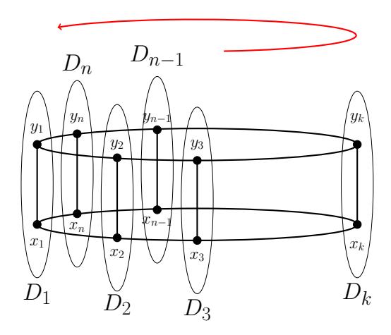
Figure 2. Labelling of vertices in \(P_2 \square C_n\)

Lemma 4.3. For \(n \ge 3\),

\[\gamma_c(P_2 \square C_n) = \begin{cases} 2, & \text{if } n = 3, \\ n, & \text{if } n > 3. \end{cases}\]

Proof. The lemma is trivially true for n=3. For n>3, clearly \(\{x_1,x_2,\ldots,x_n\}\) is a connected dominating set of \(P_2\square C_n\) and hence \(\gamma_c(P_2\square C_n)\leq n\). Suppose there exists a connected dominating set S with n-1 vertices. Since there are n columns \(D_1,D_2,\ldots,D_n\), then \(D_i\cap S=\emptyset\) for some \(i\in\{1,2,\ldots,n\}\).

Case 1: [Either \(D_{i-1}\) or \(D_{i+1}\) contains no vertices from S.] Let \(D_{i-1} \cap S = \emptyset\). Then both \(D_{i+1} \subset S\) and \(D_{i-2} \subset S\). Thus other n-5 vertices of S appear in n-4 columns \(D_1, D_2, \ldots, D_{i-3}, D_{i+2}, \ldots, D_n\). Thus there exists \(j \in \{1, 2, \ldots, i-3, i+2, \ldots, n\}\) such that \(D_j \cap S = \emptyset\). This implies that there does not exist any path from \(x_{i+1}\) to \(x_{i-2}\) in \(\langle S \rangle\) which is a contradiction to the connectedness of \(\langle S \rangle\). The case for \(D_{i+1} \cap S = \emptyset\) is similar.

Case 2: [Both \(D_{i-1}\) and \(D_{i+1}\) contains at least one vertex from S.] As there are two vertices in both \(D_{i-1}\) and \(D_{i+1}\), 4 possibilities are there:

Case 2A: \([x_{i-1}, y_{i+1} \in S]\) Since \(D_i \cap S = \emptyset\), the shortest path joining \(x_{i-1}\) and \(y_{i+1}\) should pass through at least one vertex of each \(D_k\) for \(k \in \{1, 2, ..., i-2, i+2, ..., n\}\) and since \(\langle S \rangle\) in connected, at least one \(D_k\) contains two vertices \(x_k\) and \(y_k\). This makes the total count of vertices to be n which is more than n-1 and hence a contradiction.

Case 2B: \([x_{i+1}, y_{i-1} \in S]\) Same as Case 2A.

Case 2C: \([x_{i-1}, x_{i+1} \in S]\) In this case, to dominate \(y_i\), at least one of \(y_{i-1}\) and \(y_{i+1}\) belong to S. Without loss of generality, let \(y_{i-1} \in S\). Thus \(D_{i-1} \subset S\) and \(x_{i+1} \in S\). Therefore, other n-4 vertices of S appears in the n-3 columns \(D_1, D_2, \ldots, D_{i-2}, D_{i+1}, D_{i+2}, \ldots, D_n\). Thus \(\exists j \in \{1, 2, \ldots, i-2, i+2, \ldots, n\}\) such that \(D_j \cap S = \emptyset\). As \(D_i\) and \(D_j\) are not consecutive columns, there does not exist any path joining \(x_{i-1}\) and \(x_{i+1}\) in \(\langle S \rangle\). This implies \(\langle S \rangle\) is disconnected which is a contradiction.

Case 2D: \([y_{i-1}, y_{i+1} \in S]\) Same as Case 2C.

Combining all the cases, we see that \(P_2 \square C_n\) can not have a connected dominating set of cardinality n-1 and hence \(\gamma_c(P_2 \square C_n) = n\) for \(n \ge 4\).

Theorem 4.7. For \(n \geq 3\),

\[\tau_c(P_2 \square C_n) = \begin{cases} 3, & \text{if } n = 3, \\ 30, & \text{if } n = 4, \text{ and } \\ 2(n^2 + 1), & \text{if } n > 4. \end{cases}\]

and for \(v \in V(P_2 \square C_n)\) and \(n \ge 3\),

\[CDV(v) = \begin{cases} 1, & \text{if } n = 3, \\ 15, & \text{if } n = 4, \text{ and } \\ n^2 + 1, & \text{if } n > 4. \end{cases}\]

Proof. First, we deal with the case when n=3. In this case, the only \(3 \gamma_c\)-sets are \(\{x_1,y_1\}, \{x_2,y_2\}\) and \(\{x_3,y_3\}\). Thus \(\tau_c=3\) and CDV(v)=1 for each vertex v in \(V(P_2\square C_3)\).

Now, we deal with the case when n > 3. Let S be a \(\gamma_c\)-set of \(P_2 \square C_n\) of cardinality n.

Case 1: [Each \(D_i\) contains one element of S.] Let \(x_1 \in D_1 \cap S\). We claim that \(y_i \notin S\), for all i. If possible, let \(y_i \in S\) for some \(i \in \{1, 2, \dots, n\}\). As \(\langle S \rangle\) is connected, there exists a path joining \(x_1\) and \(y_i\) in \(\langle S \rangle\). However, that path will contain \(x_j\) and \(y_j\) as consecutive vertices for some j. Thus \(D_j\) contains two vertices in S, a contradiction. Thus \(S = \{x_1, x_2, \dots, x_n\}\). Similarly, \(y_1 \in D_1 \cap S\) implies \(S = \{y_1, y_2, \dots, y_n\}\).

Case 2: [There exists at least one \(D_i\) with no element of S.]

Case 2A:[There exists more than one \(D_i\)'s with no element of S.] We first note that if the number of columns not intersecting S is more than 2, then \(\langle S \rangle\) is disconnected. Thus, let \(D_i\) and \(D_j\) be two columns which do not intersect S. As \(\langle S \rangle\) is connected, \(D_i\) and \(D_j\) are consecutive columns, i.e., let the two columns be \(D_i\) and \(D_{i+1}\). Then \(D_{i-1} \subset S\) and \(D_{i+2} \subset S\). Thus other

^&lt;sup>2</sup>Note that \(D_{i+1}\) has one vertex \(x_{i+1}\) in S, but it is also included in the list of n-3 columns as \(y_{i+1}\) may belong to S.

n-4 (provided n>4) vertices of S appears in n-4 columns \(D_1,D_2,\ldots,D_{i-2},D_{i+3},\ldots,D_n\). Since \(\langle S \rangle\) is connected, each of these n-4 columns contains exactly on element of S. Moreover to maintain connectedness of \(\langle S \rangle\), either all the \(x_i\)'s or all the \(y_i\)'s of these n-4 columns belong to S. Thus, S is of the form \(\{y_{i+2}, x_{i+2}, x_{i+3}, \dots, x_n, x_1, x_2, \dots, x_{i-1}, y_{i-1}\}\) or of the form \(\{x_{i+2}, y_{i+2}, y_{i+3}, \dots, y_n, y_1, y_2, \dots, y_{i-1}, x_{i-1}\}.\)

However, if n = 4, the two forms of S given above are identical, i.e., \(S = \{x_{i+2}, y_{i+2}, y_{i-1}, x_{i-1}\}.\)Case 2B:[There exists exactly one \(D_i\) with no element of S.] Let \(D_i \cap S = \emptyset\). Thus, to dominate \(x_i, y_i\), exactly one of the following cases should occur.

Case 2B(i): \([x_{i-1}, y_{i-1} \in S]\). In this case, the other n-2 vertices of S appears in the n-2 columns \(\{D_1, D_2, \dots, D_{i-2}, D_{i+1}, \dots, D_n\}\). Moreover, as \(D_i\) is the only column that does not intersect S, each of the n-2 columns contains exactly one element from S. Let \(x_1 \in S\). Then to preserve connectedness of \(\langle S \rangle\), \(S = \{y_{i-1}, x_{i-1}, x_{i-2}, \dots, x_1, x_n, \dots, x_{i+1}\}\). Similarly, if \(y_1 \in S\), then \(S = \{x_{i-1}, y_{i-1}, y_{i-2}, \dots, y_1, y_n, \dots, y_{i+1}\}.\)

Case 2B(ii): \([x_{i+1}, y_{i+1} \in S]\). Similar to that of Case-2B(i). In this case, either \(\text{[rumus tidak dapat ditampilkan dengan baik — lihat PDF asli]}\)\(x_{i+2}, \ldots, x_n, x_1, \ldots, x_{i-1}\) or \(S = \{x_{i+1}, y_{i+1}, y_{i+2}, \ldots, y_n, y_1, \ldots, y_{i-1}\}.\)

Case 2B(iii): \([x_{i-1}, y_{i+1} \in S.]\) Similarly, in this case, \(\exists j \in \{1, 2, \dots, i-2, i+2, \dots, n\}\) such that \(S = \{y_{i+1}, y_{i+2}, \dots, y_i, x_i, \dots, x_{i-2}, x_{i-1}\}.\)

Case 2B(iv): \([x_{i+1}, y_{i-1} \in S.]\) Similarly, in this case, \(\exists j \in \{1, 2, \dots, i-2, i+2, \dots, n\}\) such that \(S = \{x_{i+1}, x_{i+2}, \dots, x_j, y_j, \dots y_{i-2}, y_{i-1}\}.\)

While classifying the \(\gamma_c\)-sets, we see that there are mainly three types of \(\gamma_c\)-sets of \(P_2 \square C_n\):

• The types given by Case-1: \(S = \{x_1, x_2, \dots, x_n\}\) and \(S = \{y_1, y_2, \dots, y_n\}\). Thus total number of \(\gamma_c\)-sets of this type is 2.
• The types given by Case-2A: S's which do not contain vertices from two consecutive columns \(D_i\) and \(D_{i+1}\). As the number of ways in which we can drop two consecutive columns is n, the total number of \(\gamma_c\)-sets of this type is equal to 2n, if n > 4 and is equal to 4, if n = 4.
• The types given by Case-2B: In Case-2B(i), we have two choices for S for each i. Thus Case-2B(i) contribute 2n many \(\gamma_c\)-sets. Similarly, Case-2B(ii) contribute 2n many \(\gamma_c\)-sets. In Case-2B(iii), we have n choices for i and n-3 choices for j. Thus Case-2B(iii) contribute n(n-3) many \(\gamma_c\)-sets. Similarly, Case-2B(ii) contribute n(n-3) many \(\gamma_c\)-sets.

Thus the total number of distinct \(\gamma_c\)-sets of \(P_2 \square C_n\) is \(2(n^2+1)\), i.e., \(\tau_c=2(n^2+1)\), if n>4. If n=4, then \(\tau_c=30\). Now, as \(P_2\square C_n\) is vertex transitive, CDV(u)=CDV(v) for all \(u,v\in\)\(P_2\square C_n\). Hence, by continuous analogue of Proposition 2.1, we have \(2n \cdot CDV(v) = 2n(n^2 + 1)\), i.e., \(CDV(v) = n^2 + 1\) for n > 4. For n = 4, by Proposition 2.1, we have \(8 \cdot CDV(v) = 4 \cdot 30\), i.e., CDV(v) = 15.

Hence, the theorem follows.

Acknowledgement

The author is grateful to the anonymous referee for providing fruitful suggestions and pointing out a few mistakes in the original manuscript. The funding of DST-SERB-SRG Sanction no. SRG/2019/000475, Govt. of India is acknowledged.

References

• [1] E.J. Cockayne, R.M. Dawes, and S.T. Hedetniemi, Total domination in graphs, Networks 10 (3) (1980), 211–219.
• [2] E.J. Cockayne, M.A. Henning, and C.M. Mynhardt, Vertices contained in all or in no minimum total dominating set of a tree, Discrete Math. 260 (2003), 37–44.
• [3] A. Das, R.C. Laskar, and N.J. Rad, On α-domination in graphs, Graphs Combin. 34 (2018), 193–205.
• [4] A. Das, Partial domination in graphs, Iran. J. Sci. Technol. Trans. A Sci. 43 (2019),1713– 1718.
• [5] A. Das, Coefficient of domination in graph, Discrete Math. Algorithms Appl. 9(2) (2017), 1750018.
• [6] I.S. Hamid, S. Balamurugan, and A. Navaneethakrishnan, A note on isolate domination, Electron. J. Graph Theory Appl. 4 (1) (2016), 94–100.
• [7] T.W. Haynes, S.T. Hedetniemi, and P.J. Slater, Fundamentals of domination in graphs, Marcel Dekker Inc., 1998.
• [8] T.W. Haynes, S.T. Hedetniemi, and P.J. Slater (eds), Domination in Graphs: Advanced Topics, Marcel Dekker Inc., 1998.
• [9] C.X. Kang, Total domination value in graphs, Util. Math. 95 (2014), 263–279.
• [10] N. Meddah and M. Blidia, Vertices contained in all or in no minimum k-dominating set of a tree, AKCE Int. J. Graphs Comb. 11 (1) (2014), 105–113.
• [11] D.A. Mojdeh, S.R. Musawi, and E. Nazari, On the distance domination number of bipartite graphs, Electron. J. Graph Theory Appl. 8 (2) (2020), 353–364.
• [12] C.M. Mynhardt, Vertices contained in every minimum dominating set of a tree, J. Graph Theory 31 (1999), 163–177.
• [13] E. Sampathkumar, and H.B. Walikar, The connected domination number of a graph, J. Math. Phy. Sci. 13 (6) (1979), 607–613.
• [14] D.B. West, Introduction to Graph Theory, Prentice Hall, 2001.
• [15] E. Yi, Domination value in graphs, Contrib. Discrete Math. 7 (2) (2012), 30–43.
• [16] E. Yi: Domination value in P2Pⁿ and P2Cn, J. Combin. Math. Combin. Comput. 82 (2012), 59–75.