Alf Kimms
Chair of Logistics and Operations Research, Mercator School of Management, University of Duisburg–Essen, Lotharstr. 65, 47048 Duisburg, Germany
alf.kimms@uni–due.de
Paul Erdos said about the ¨ 3x + 1 problem, "Mathematics is not yet ready for such problems". And he is seemingly right. Although we cannot solve this problem either, we provide some results about its structure. The so–called Collatz graph is iteratively transformed into a sequence of graphs by making use of some hidden structure information. It turns out that the transformation of graphs corresponds to a sequence of sets of numbers. It is shown that if the union of these number sets were equal to the set of integers greater than one, the famous Collatz conjecture would be true.
Keywords: Collatz graph, graph transformation, 3x + 1 problem, Collatz problem, Syracuse problem, Kakutani's problem, Haase's algorithm, Ulam's problem, Thwaites' problem, hailstone numbers Mathematics Subject Classification : 11B83, 05C90
DOI: 10.5614/ejgta.2021.9.1.14
1. Basics of the 3x + 1 Problem
The so–called 3x + 1 problem is a problem in number theory that has been around for decades. The exact origin is reported to be obscure and seems to go back to the 1930's, but for sure it has been known to the community since 1952 (see Lagarias, 1985, and the references therein). Up to now, the problem is considered to be unsolved, although many noble mathematicians have tried to solve it. Depending on who worked on it or where it has been addressed, the problem became known under several different names like, e.g., the Collatz conjecture, the Syracuse problem, Kakutani's problem, Haase's algorithm, Ulam's problem, and the Thwaites problem.
Received: 19 May 2017, Revised: 15 January 2021, Accepted: 12 February 2021.
The 3x+1 problem can be stated in a very simple manner: Given a positive integer \(x_0\), consider the following sequence of positive integers:
\[x_{i+1} = \begin{cases} x_i/2, & \text{if } x_i \text{ is even,} \\ 3x_i + 1, & \text{if } x_i \text{ is odd.} \end{cases}\]
As an example, consider \(x_0 = 9\). We then get the (infinite) sequence given in Table 1. Some authors mention that the sequence of \(x_i\)-values behaves somewhat "randomly" (e.g. Lagarias, 1985, states that it simulates "random" behavior) which might be a reason for the missing proof. Because of that, the numbers in the sequence are sometimes called hailstone numbers because they seem to behave as erraticly as hailstones in a cloud.
| i = | 0 | 1 | 2 | 3 | 4 | 5 | 6 | 7 | 8 | 9 | 10 | 11 | 12 | 13 | 14 | 15 | 16 | 17 | 18 | 19 | ••• |
|---|---|---|---|---|---|---|---|---|---|---|---|---|---|---|---|---|---|---|---|---|---|
| \(x_i =\) | 9 | 28 | 14 | 7 | 22 | 11 | 34 | 17 | 52 | 26 | 13 | 40 | 20 | 10 | 5 | 16 | 8 | 4 | 2 | 1 |
Table 1. The sequence with initial value \(x_0 = 9\)
Note, the sequence has reached the value one after a finite number of iterations. Those readers who are not familiar with the problem are invited to try different \(x_0\) values to check whether or not the value one is among the numbers in the sequence. Sometimes a little patience is required as for \(x_0 = 27\), for example.
If there is a need to emphasize the rules that are applied to construct the sequence, we will use a notation similar to
\[9 \xrightarrow{3x+1} 28 \xrightarrow{x/2} 14 \xrightarrow{x/2} 7 \xrightarrow{3x+1} 22 \xrightarrow{x/2} \dots \xrightarrow{x/2} 1.\]
Often a graph is drawn to illustrate the problem. It is constructed as follows and it is referred to as the Collatz graph: Numbers are represented by nodes. An arc points from a number \(x_i\) to a number \(x_{i+1}\) if and only if \(x_{i+1}\) is the unique number that immediately follows \(x_i\) in the sequence defined above. While this is sufficient to draw the graph, one should note that there is a very systematic way to construct the graph.
Since prime factorization is unique, for each number x that is odd there is a sequence of even numbers that precedes x. For example, we have \(5 \leftarrow 10 \leftarrow 20 \leftarrow 40 \leftarrow \ldots\) in the graph. We call this the x-spine and the example just given shows the 5-spine. The number x of the x-spine will be called the head of the spine. Since we will modify this graph later on and find out that there are similar substructures in the modified graphs, we will refer to such x-spines more precisely as x-level m-spines, where m denotes the number of modifications that were done meanwhile unless it is clear from the context what level we talk about. Initially, we are at level 0 and \(5 \leftarrow 10 \leftarrow 20 \leftarrow 40 \leftarrow \ldots\) would consequently be the 5-level 0-spine. In a similar manner, we call the graphs level m-graphs so that the Collatz graph is the level 0-graph.
Furthermore, in the Collatz graph there is an arc from every odd number x to the even number 3x+1, i.e., the head x of the x-spine is connected to an even number that occurs in another spine (there is one exception: 1 connects to 4 which is in the 1-spine). In our example, 5 connects to 16. We can now arrange the x-spines in such a way (see Table 2) that each x-spine forms a column, the step \(x \to x/2\) (if x is even) means moving vertically upwards, and the step \(x \to 3x+1\) (if x
is odd) means moving horizontally leftwards to the next number. Table 2 also illustrates how we proceed through the graph given x0 = 9 (compare Table 1).
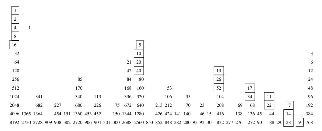
Table 2. An illustration of (parts of) the Collatz graph (the level 0–graph)
As of May 2020 it has been verified that at least for all positive integer starting values up to 268 we do indeed reach the value one (see the web sites http://sweet.ua.pt/tos/3x+1.html maintained by Thomas Oliveira e Silva and http://www.ericr.nl/wondrous/ maintained by Eric Roosendaal, respectively, for recent computational results). This leads to the so–called Collatz conjecture:
For any positive integer x0, the corresponding sequence of xi–values will reach the value one in a finite number of steps.
No accepted proof for this conjecture is available yet.
Trying to grasp the nature of the problem, one can draw a graph that illustrates the fixed point iteration given a starting value x0. Figure 1, for example, shows what is going on when we start with x0 = 9.
There exists a cycle 4 ! 2 ! 1 ! 4 ! ... which contains the value one. But it is not clear whether or not other cycles exist which may not contain the value one and which may lead to infinite looping. Also, it might be that a sequence diverges in the sense that an infinite number of different numbers is enumerated without getting to the value one.
Nevertheless, many insightful results have been gained. Jeffrey Lagarias eagerly collected papers on that problem and published surveys (Lagarias, 1985) and an edited volume of important papers (Lagarias, 2010) which makes him become a historian of that problem. Because his collection of literature is extremely comprehensive, we do not review here the many papers that exist and refer to the reviews published by Lagarias instead (updated versions are available online: Lagarias, 2011 and 2012). The book by Wirsching (1998) also contains a lot of material. Chamberland (2003) provides an overview of major trends. The work that comes closest to our paper is by Andaloro (2002) who investigates the connectivity of the Collatz graph.
With this paper, we contribute to the problem by revealing some properties of the structure of the problem which, to the best of our knowledge, have not been used before. The paper is
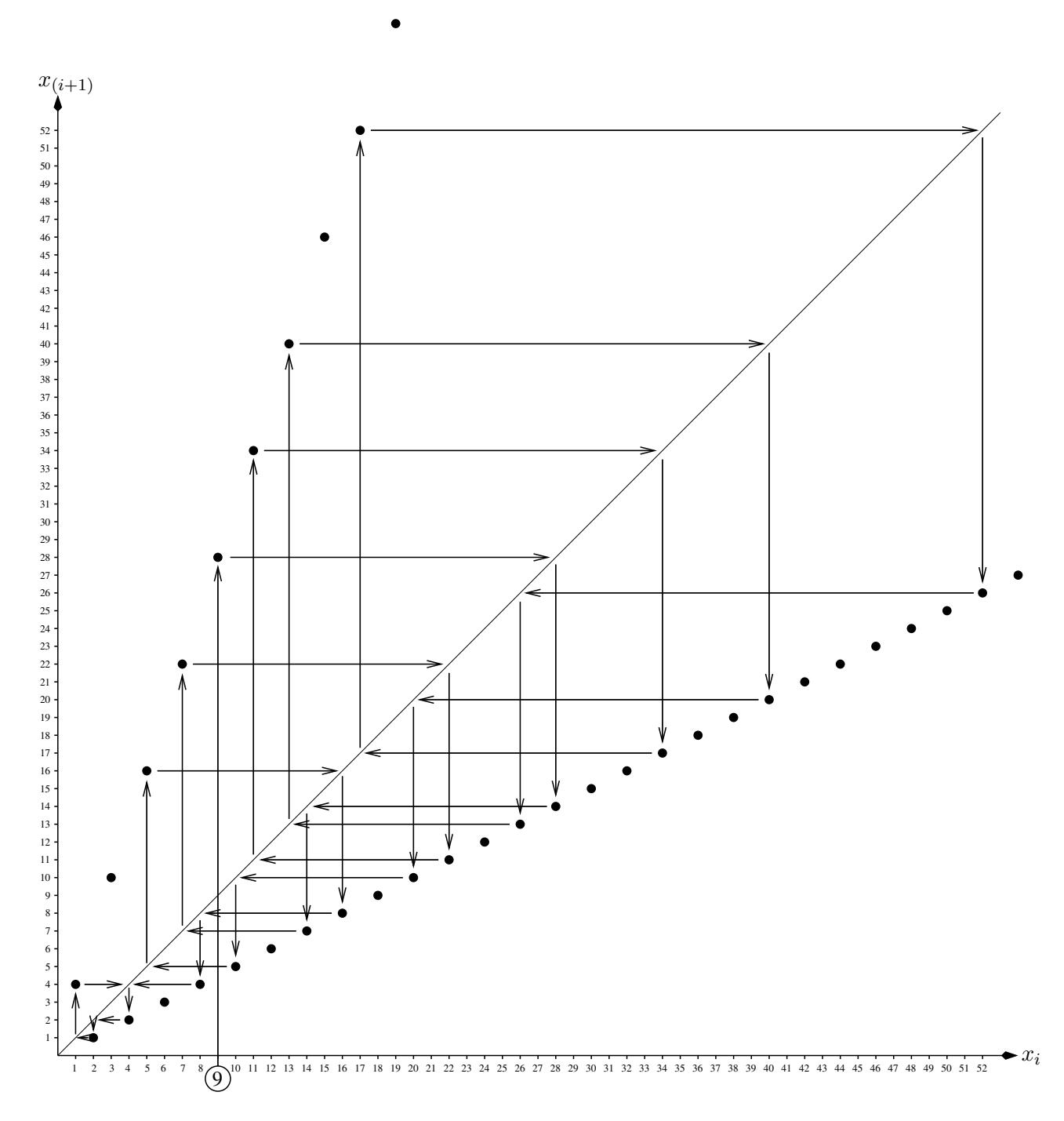
Figure 1. The fixed point iteration with x0 = 9
organized as follows: Section 2 shows a systematic way to reduce the 3x+1 problem to a problem with a reduced set of numbers. While not only the original problem can be represented as a graph (the Collatz graph), the reduced problem can be represented by a graph, too. We show that there is a very systematic way of transforming one graph into the other. In Section 3, we will demonstrate that this systematic process can be iterated to get a sequence of graphs. While doing so, the set of numbers that are contained in these graphs is reduced from one level to the next. This allows us to reformulate the Collatz conjecture based on the numbers that are eliminated. Section 4 demonstrates how the eliminated numbers can be computed in a systematic manner. A final Section 5 concludes the paper and points to some conjectures that we have and that may inspire future work.
2. Sequences of Odds
By studying the numbers in the Collatz graph carefully, we can derive some properties that relate certain numbers to each other. This will be done in this section and we will show that the sequence of \(x_i\)-values can be replaced by a sequence of \(y_j\)-values where most of the \(y_j\)-numbers are odd and only the starting value \(y_0\) might be even.
Case 1. Let us begin with assuming \(x_i\) being an even number. Since there is a unique prime factorization, an even \(x_i\) is of the form \(x_i = 2^k P\) with \(k \ge 1\) and P odd. Thus, the sequence would evolve from \(x_i\) to \(x_{i+k} = P\) by repeatedly divide the incumbent number by 2:
\[x_i = 2^k P \xrightarrow{x/2} x_{i+1} \xrightarrow{x/2} \dots \xrightarrow{x/2} x_{i+k} = P.\]
That means that we can consider a sequence \(y_j = x_i\) and \(y_{j+1} = P\) in order to find out whether or not we can eventually reach the value one. As an example, consider \(x_i = 40 = 2^3 \cdot 5\). We will jump to 5 then (see Table 2) and Case 1 is an obvious shortcut.
Case 2. Let us now consider an odd number x. In the Collatz graph x connects to the even number 3x+1 which belongs to some spine. In that spine 3x+1 is preceded by 6x+2 which in turn is preceded by 12x+4. It is important to note that there cannot be any odd integer number x' which connects to 6x+2 in the Collatz graph. This is easy to see by contradiction. Assume there is an odd integer x' such that 3x'+1=6x+2 holds. This implies \(x'=2x+\frac{1}{3}\) which contradicts to the assumption that x' is an integer. On the other hand there exists an odd integer x'' so that 3x''+1=12x+4. The value of x'' is x''=4x+1. We can turn this round to observe that if we face an odd integer \(x_i\) such that \(x_i-1\) can be divided by 4 giving a result that is an odd integer, we can jump to \((x_i-1)/4\) instead. The reason is that both, \(x_i\) and \((x_i-1)/4\), are connected to the very same spine so that for the task of finding out whether or not we reach the value one in the sequence, a starting point \((x_i-1)/4\) is equivalent to \(x_i\) (if \((x_i-1)/4\) is an odd integer). This allows us to define \(y_j=x_i\) and \(y_{j+1}=(y_j-1)/4\) in such circumstances. Figure 2 illustrates this case. Consider the example \(x_i=21\) which is connected to the 1-spine. Instead of 21, we will consider (21-1)/4=5 which is connected to the 1-spine, too (see Table 2).
In Case 3 and 4, finally, assume \(x_i\) is an odd number, i.e. \(x_i = 2n + 1\) with n being a non-negative integer, and \((x_i - 1)/4\) is not an odd integer. In such a case, the next number in the
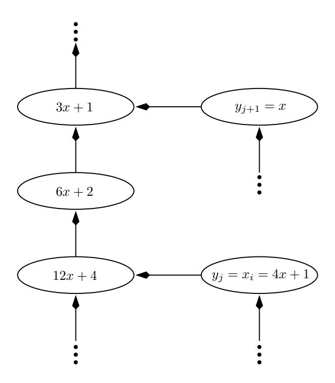
Figure 2. The case where xi and (xi 1)/4 are odd
sequence is defined to be xi+1 = 3xi + 1 and it is clear that xi+1 is even because xi+1 = 3(2n + 1) + 1 = 6n + 4. Depending on n two cases exist.
Case 3. n is even. For example, consider xi =9=2 · 4+1 (n = 4 is even). If n is even it can be written as n = 2n0 with n0 being a non–negative integer. Thus, we have xi = 4n0 + 1. Recall that we have assumed that (xi 1)/4 is not odd. Consequently, n0 must be even. It turns out that xi+1 = 6n + 4 = 12n0 + 4. xi+1 can now be divided by 4 to get xi+3 = 3n0 + 1. Since n0 is even, xi+3 is odd and we can define yj = xi and yj+1 = (3yj + 1)/4. Compare Table 2 to check that we can take a shortcut and jump from 9 to (3·9+1)/4=7. To repeat how this relates to the definition of the sequence, note that the following subsequence was considered:
\[x_i \xrightarrow{3x+1} x_{i+1} \xrightarrow{x/2} x_{i+2} \xrightarrow{x/2} x_{i+3}.\]
Case 4. n is odd. As an example, one may consider xi = 11 = 2 · 5+1 (n = 5 is odd). In that case n is of the form n = 2n0 + 1 with n0 being a non–negative integer and xi = 4n0 + 3. Applying the definition of the sequence we get xi+1 = 6(2n0 + 1) + 4 = 12n0 + 10. And xi+2 = 6n0 + 5 turns out to be an odd number. With this observation, we can define yj = xi and yj+1 = (3yj + 1)/2. Again, we can refer to Table 2 as an example to see that once we have reached 11 we can go to (3 · 11 + 1)/2 = 17 next. The following subsequence illustrates what we did:
\[x_i \xrightarrow{3x+1} x_{i+1} \xrightarrow{x/2} x_{i+2}.\]
In summary we have proven that, given a positive integer value \(y_0 = x_0\), it is sufficient to investigate the following sequence of positive integers in order to find out if the 3x + 1 problem eventually reaches the value one in all cases:
\[\text{[rumus tidak dapat ditampilkan dengan baik — lihat PDF asli]}\]
The question is, given any positive integer \(y_0 = x_0\), does the sequence of \(y_j\)-values eventually reach the value one? Appendix Appendix A provides details for the odd numbers \(y_j\) from 1 to 767.
Since only \(y_0\) might be even, we can focus on odd numbers. The possible sequences of \(y_j\)-values can be represented as an infinite graph, the level 1-graph, as shown in Table 3. For a each odd number y for which (y-1)/4 is not an odd integer, there is a set of odd numbers which result from calculating 4y+1 repeatedly (compare Figure 2). \(9 \leftarrow 37 \leftarrow 149 \leftarrow \ldots\) is an example. These numbers are connected in monotonic order. In Table 3 you will see these numbers as columns to form a level 1-spine. The example \(9 \leftarrow 37 \leftarrow 149 \leftarrow \ldots\) is the 9-level 1-spine. Each odd number y where (y-1)/4 is not an odd integer (such a number is the head of a level 1-spine; see Table 3) is connected to either (3y+1)/4 (if this is an odd number) or (3y+1)/2 (in Figure 3 you have to move horizontally to the next number in such cases). As an example, for \(y_0 = 9\) we get the following sequence:
\[9 \xrightarrow{(3y+1)/4} 7 \xrightarrow{(3y+1)/2} 11 \xrightarrow{(3y+1)/2} 17 \xrightarrow{(3y+1)/4} 13 \xrightarrow{(y-1)/4} 3 \xrightarrow{(3y+1)/2} 5 \xrightarrow{(y-1)/4} 1.\]
Table 3. The sequences of odd numbers can be represented by a graph, the level 1-graph
It might be worth to note that hidden in the definition of the sequence of \(y_j\)-values there is a systematic pattern for the sequence of odd numbers. Remember that each odd number \(y_j\) can be represented as \(y_j = 2n + 1\) where n is a non-negative integer. The rule that determines what number comes next in the sequence is clearly defined above. So, let us first look at those odd numbers \(y_j\) for which \((y_j - 1)/4\) is an odd integer (see Table 4). Let \(n_a\) be a counter of these numbers in increasing order starting with zero. The counter \(n_a\) relates to n in the following way: \(n = 4n_a + 2\). These numbers have the form \(y_j = 8n_a + 5\) and the odd number that follows in the sequence is \(y_{j+1} = 2n_a + 1\). The distance between \(y_j\) and \(y_{j+1}\) in terms of n is \(\Delta n = -(3n_a + 2)\).
In a similar manner we can study the structure of those odd numbers \(y_j\) for which the subsequent number \(y_{j+1}\) is calculated by the rule \((3y_j + 1)/4\) (see Table 5). Let \(n_b\) be a counter of these numbers. The relation to n is \(n = 4n_b\). We have \(y_j = 8n_b + 1\) and the subsequent number is
The structure of the 3x + 1 problem | Alf Kimms
yj = 5 13 21 29 37 45 53 ...
na = 0 1 2 3 4 5 6 ...
n = 2 6 10 14 18 22 26 ...
yj+1 = 1 3 5 7 9 11 13 ...
Table 4. Odd numbers yj where the next number in the sequence is (yj 1)/4
yj+1 = yj 2nb. The distance between these two numbers is n = nb.
yj = 1 9 17 25 33 41 49 ...
nb = 0 1 2 3 4 5 6 ...
n = 0 4 8 12 16 20 24 ...
yj+1 = 1 7 13 19 25 31 37 ...
Table 5. Odd numbers yj where the next number in the sequence is (3yj + 1)/4
Finally, we look at odd numbers yj where the follower yj+1 is defined to be (3yj + 1)/2 (see Table 6). Let nc be a counter for those numbers so that we have n = 2nc + 1. yj is of the form yj = 4nc + 3 and yj+1 = yj + 2(nc + 1). The distance is n = nc + 1.
yj = 3 7 11 15 19 23 27 ...
nc = 0 1 2 3 4 5 6 ...
n = 1 3 5 7 9 11 13 ...
yj+1 = 5 11 17 23 29 35 41 ...
Table 6. Odd numbers yj where the next number in the sequence is (3yj + 1)/2
Figure 3 illustrates the relationships between the odd numbers and indicates which number follows a particular number.
3. Level m–Graphs and the Collatz Conjecture
In this section we will carefully study what the transformation of the level 0–graph to the level 1–graph, which was described in the previous section, really does. This process can then be iterated so that we will learn something about the problem that allows us to reformulate the Collatz conjecture.
To start with, let us have a look at the graph at a level m. It consists of level m–spines where the head of each spine is connected to some other spine. Figure 4 illustrates the structure of the level m–graph (compare Table 2 for an illustration of the level 0–graph). Note that it will turn out to be convenient to consider several copies of the number one in the graph (in the level 0–graph, for instance, we have one node x1 = 1 for the number one because x = 2 results in x1 = 1, we have a second node for the number one because x2 = 1 yields x = 4 which means that the node
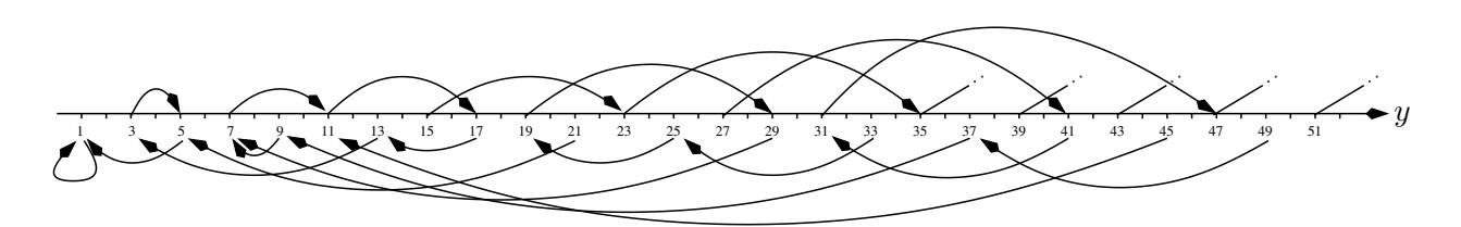
Figure 3. An illustration of the internal structure of the sequence of odds
for \(x^2 = 1\) connects to the \(x^1\)-spine, we have a third node for the number one because \(x^3 = 1\) connects to the \(x^2 = 1\)-spine, and so on).
Figure 4. Sketch of the level m-graph
There are certain relationships among the numbers in the level m-graph that can be described by distinct functions (see Figure 5) where the domains and the codomains are subsets of the set \(\mathbb{N} := \{1,2,3,\ldots\}\) of positive integers: First of all, there is a function \(s_m : \mathbb{N} \to \mathbb{N}\) that is applied whenever we move along a spine from one number to another. A second function \(g_m : \mathbb{N} \to \mathbb{N}\) describes what happens when we jump from the head of a spine to the spine this head number is connected to. The head nodes of all the spines which are connected to a common spine can be related to each other by a function \(f_m : \mathbb{N} \to \mathbb{N}\). And finally, we can derive a function \(h_m : \mathbb{N} \to \mathbb{N}\) that describes the relationship between the last node that connects to a particular spine to the head of that spine.
For the level 0-graph \(s_0\) is defined to be
\[s_0: \mathbb{N} \to \mathbb{N}, s_0(x) = x/2,\]
and the domain of \(s_0\) is the set of even integers, i.e. \(dom(s_0) = \mathbb{N}^{even} := \{x \in \mathbb{N} | x \text{ is even}\}.\) The
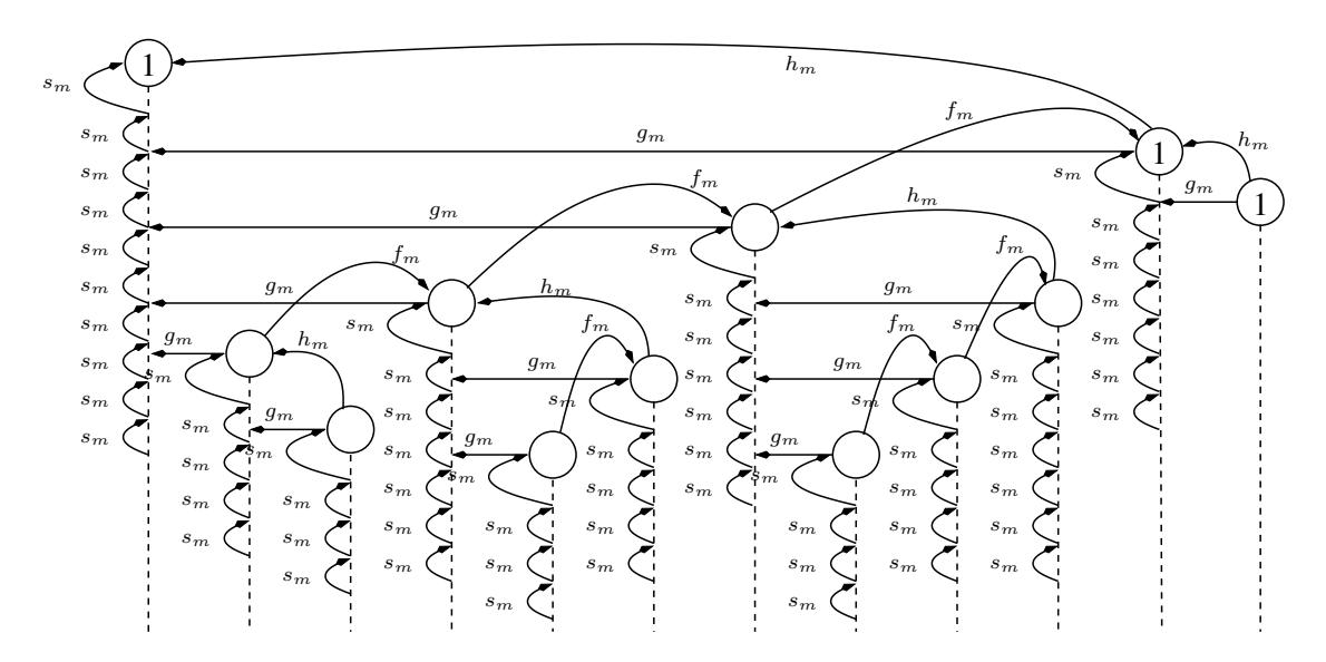
Figure 5. Functions in the level m–graph that relate nodes
function \(g_0\) is defined as
\[g_0: \mathbb{N} \to \mathbb{N}, g_0(x) = 3x + 1,\]
the domain is the set of odd integers, i.e. \(dom(g_0) = \mathbb{N} \backslash dom(s_0) = \mathbb{N}^{odd} := \{x \in \mathbb{N} | x \text{ is odd}\},\) and the codomain is the set of even integers, i.e. \(codom(g_0) = \mathbb{N}^{even}\). By construction, a composition of \(s_m\) and \(g_m\) defines \(f_m\) and \(h_m\). To be precise,
\[f_m(x) = g_m^{-1} \circ s_m^{k_x} \circ g_m(x)\]
for a proper value \(k_x \ge 1\) that may or may not depend on the argument x (\(g_m^{-1}\) denotes the inverse of \(g_m\)). The previous section taught us (compare Case 2 and Figure 2) that
\[f_0(x) = (x-1)/4\], if \((x-1)/4 \in \mathbb{N}^{odd}\).
Regarding \(h_m\) we have
\[h_m(x) = s_m^{k_x} \circ g_m(x)\]
where \(s_m^k = \underbrace{s_m \circ \ldots \circ s_m}_{\times k_x}\) and \(k_x \ge 0\) is appropriately chosen possibly depending on the argument
x. For m=0 we have already derived in the previous section (see Cases 3 and 4) that
\[h_0(x) = \begin{cases} (3x+1)/4, & \text{if } (3x+1)/4 \in \mathbb{N}^{odd} \text{ and } x \not\in dom(f_0), \\ (3x+1)/2, & \text{if } (3x+1)/2 \in \mathbb{N}^{odd} \text{ and } x \not\in dom(f_0). \end{cases}\]
Note, one is a fixed point of \(h_0\), i.e. \(h_0(1) = 1\).
Up to here we have just recalled what we know about the Collatz graph (i.e. the level 0–graph). From that we have derived the sequences of odds in the previous section using among other things
the simple insight that each even number can be reduced to an odd number by applying the function \(s_0\) repeatedly (i.e. by moving along the spine to a smaller number). In other words, those numbers which belong to \(dom(s_0)\) could have been eliminated from further consideration. Let \(\mathbb{N}_m\) be the set of numbers that are considered at level m. Initially, we have \(\mathbb{N}_0 := \mathbb{N}\). At level 1 we have \(\mathbb{N}_1 := \mathbb{N}_0 \backslash dom(s_0) = \mathbb{N}^{odd}\).
The remaining numbers (i.e. the numbers in \(\mathbb{N}_1\)) can be partially ordered and arranged in a graph (see Table 3). The way this graph is constructed can be generalized as follows: Let \(\mathbb{N}_m\) be the set of numbers that are considered at level m. Given the level m-graph (and, thus, the functions \(s_m\), \(g_m\), \(f_m\), and \(h_m\)) the level (m+1)-graph consists of level (m+1)-spines which are made out of those numbers that are linked by the function \(f_m\). The set \(\mathbb{N}_{m+1}\) therefore is \(\mathbb{N}_{m+1} := \mathbb{N}_m \backslash dom(s_m)\). The number to which the head of such a level (m+1)-spine is connected to in the level (m+1)-graph is determined by the function \(h_m\). Numbers to which the function \(s_m\) is applied do not show up any more in the level (m+1)-graph. Again, we refer to Tables 2 and 3 where the level 0-graph and the level 1-graph are illustrated, respectively. Additionally, Figure 6 highlights some key numbers to emphasize the underlying idea of the graph transformation. To wrap up, the resulting functions for the level (m+1)-graph are:
\[s_{m+1} = f_m\]\[g_{m+1} = h_m\]
By construction, there is a 1-spine in the level (m+1)-graph (and in all graphs with a lower level). The functions \(f_{m+1}\) and \(h_{m+1}\) can then be derived using the basic cooking rule from above, i.e.
\[f_{m+1}(x) = g_{m+1}^{-1} \circ s_{m+1}^{k_x} \circ g_{m+1}(x)\] with \(k_x \ge 1\)
and
\[h_{m+1}(x) = s_{m+1}^{k_x} \circ g_{m+1}(x)\] with \(k_x \ge 0\),
while taking into account that \(dom(f_{m+1}) \subset \mathbb{N}_{m+2} = \mathbb{N}_{m+1} \setminus dom(s_{m+1})\), \(codom(f_{m+1}) = \mathbb{N}_{m+2} \subset \mathbb{N}_{m+1}\), \(dom(h_{m+1}) = \mathbb{N}_{m+1} \setminus (dom(s_{m+1}) \cup dom(f_{m+1}))\), and \(codom(h_{m+1}) = \mathbb{N}_{m+2} \subset \mathbb{N}_{m+1}\).
For m = 1 we get
\[\text{[rumus tidak dapat ditampilkan dengan baik — lihat PDF asli]}\]
where
\[dom(s_1) = \{x \in \mathbb{N}_1 = \mathbb{N}^{odd} | (x-1)/4 \in \mathbb{N}_1 = \mathbb{N}^{odd} \},\]
= \{5, 13, 21, 29, 37, 45, 53, 61, 69, 77, 85, 93, 101, \dots\}.
We can iterate this procedure to construct a sequence of level m-graphs. The fundamental lesson to learn is that if we can prove that all numbers included in the level (m+1)-graph reduce to the value one by applying the functions \(s_{m+1}\) and \(g_{m+1}\), we can then be sure that all numbers in the set \(\bigcup_{i=0}^m dom(s_i)\) eventually lead to the value one as well. That means to prove the Collatz
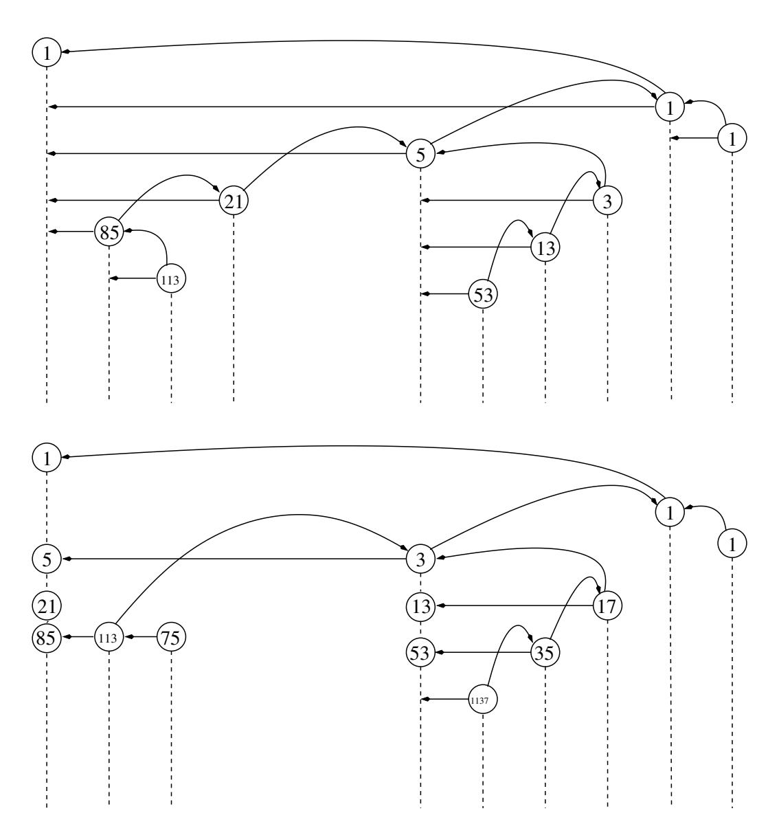
Figure 6. Transformation of the level 0–graph into the level 1–graph
conjecture it is sufficient to show that for every positive integer \(x_0\) greater than one there is a level m such that \(x_0 \in dom(s_m)\). In mathematical terms the Collatz conjecture can be reformulated as
\[\forall x_0 \in \mathbb{N} \setminus \{1\} : \exists m \ge 0 : x_0 \in dom(s_m).\]
4. The Domains of the Spine Functions
What remains to do is to determine the domains of the spine functions \(s_m\). We do this level by level. For m = 0 and m = 1 we do have some results already.
Level m = 0 (see above):
\[dom(s_0) = \mathbb{N}^{even}\]
= \(\{2, 4, 6, 8, 10, 12, 14, \ldots\}.\)
Level m = 1 (see above):
\[\overline{dom(s_1)} = \{x \in \mathbb{N}_1 = \mathbb{N}^{odd} | (x-1)/4 \in \mathbb{N}_1 = \mathbb{N}^{odd} \}, = \{5, 13, 21, 29, 37, 45, 53, 61, 69, 77, 85, 93, 101, \ldots \}.\]
For higher levels, we will need \(f_1\). We know that \(f_1\) is of the form
\[f_1(x) = g_1^{-1} \circ s_1^{k_x} \circ g_1(x)\]
where
\[\text{[rumus tidak dapat ditampilkan dengan baik — lihat PDF asli]}\]
is known from above. This is equivalent to
\[x = g_1^{-1} \circ s_1^{-k_x} \circ g_1(f_1(x)).\]
It is crucial to take into account that all intermediate results must belong to \(\mathbb{N}_1\), i.e. we must have \(g_1(f_1(x)) \in \mathbb{N}_1\), \(s_1^{-1}(g_1(f_1(x))) \in \mathbb{N}_1\) and so on (or, which is equivalent, \(g_1(x) \in \mathbb{N}_1\), \(s_1(g_1(x)) \in \mathbb{N}_1\) and so on).
Two cases can occur:
(i) \[f_1(x) \xrightarrow{g_1} (3f_1(x) + 1)/4 \xrightarrow{s_1^{-1}} 4((3f_1(x) + 1)/4) + 1 = 3f_1(x) + 2 \xrightarrow{g_1^{-1}} (2(3f_1(x) + 2) - 1)/3 = 2f_1(x) + 1\]. That is, \(f_1(x) = (x - 1)/2\).
(ii) \[f_1(x) \xrightarrow{g_1} (3f_1(x)+1)/2 \xrightarrow{s_1^{-1}} 4((3f_1(x)+1)/2) + 1 = 6f_1(x) + 3 \xrightarrow{s_1^{-1}} 4(6f_1(x)+3) + 1 = 24f_1(x) + 13 \xrightarrow{g_1^{-1}} (4(24f_1(x)+13)-1)/3 = 32f_1(x) + 17.\] That is,
\[f_1(x) = (x - 17)/32.\]
The function \(h_1\) will be needed on higher levels, too, because \(g_2 = h_1\) will be used. From the deduction of \(f_1\) we can conclude the definition of \(h_1\):
\[h_1(x) = \begin{cases} g_1(x), & \text{if } g_1(x) \notin dom(s_1), \\ ((3x+1)/4-1)/4, & \text{if } g_1(x) \in dom(s_1). \end{cases}\]
Note that the number one is a fixed point of \(h_1\), i.e. \(h_1(1) = 1\). Level m = 2:
Since \(s_2(x) = f_1(x)\) with \(x \in \mathbb{N}_2\) and \(s_2(x) \in \mathbb{N}_2\), we can determine \(dom(s_2)\) as follows: \(dom(s_2) = \{x \in \mathbb{N}_2 | (3x+1)/2 \in \mathbb{N}_1 \text{ and } ((3x+1)/2-1)/4 \in \mathbb{N}_1 \text{ and } (x-1)/2 \in \mathbb{N}_2\}\) \(\cup \{x \in \mathbb{N}_2 | (3x+1)/4 \in \mathbb{N}_1 \text{ and } ((3x+1)/4-1)/4 \in \mathbb{N}_1 \text{ and } ((3x+1)/4-1)/4 \in \mathbb{N}_1 \text{ and } ((3x+1)/4-1)/4 \in \mathbb{N}_1 \text{ and } (x-17)/32 \in \mathbb{N}_2\}\) \(= \{3,7,1/2,1/3,1/3,1/3,1/3,3/3,3/3,3/3,3/3,4/3,4/3,51,\ldots\}\) \(\cup \{49,113,1/7,241,3/3,3/3,3/3,4/3,4/3,\ldots\}.\)
Note that we have listed odd numbers \(x \in \mathbb{N}_2\) where (x-1)/2 or (x-17)/32, respectively, is odd and we then canceled out all those x-values which do not belong to \(dom(s_2)\) to emphasize that the conditions under which a number x belongs to \(dom(s_2)\) is a bit more complex than one might expect. Some examples which show why certain numbers do not belong to \(dom(s_2)\) are given here: \(11 \notin dom(s_2)\) because \((11-1)/2 = 5 \in dom(s_1) \nsubseteq \mathbb{N}_2\). \(7 \notin dom(s_2)\) because \(7 \xrightarrow{g_1} 11 \xrightarrow{s_1} (11-1)/4 \notin \mathbb{N}_1\). \(49 \notin dom(s_2)\) because \(49 \xrightarrow{g_1} 37 \xrightarrow{s_1} 9 \xrightarrow{s_1} 2 \notin \mathbb{N}_1\).
Further levels can be investigated in a similar manner. We stop here because we assume that there is in infinite sequence of levels to consider and the inductive construction of the domains of the functions \(s_m\) will not terminate.
5. Conclusion
The so-called Collatz conjecture states that the 3x+1 problem generates a sequence of numbers that will reach the value one in a finite number of steps. Many people including us believe that this is true, but no proof is available yet. As many others before, we also failed to provide a complete proof and the 3x+1 problem remains to be a mystery.
We studied the so-called Collatz graph. We suggested to transform this graph into another graph which is transformed into just another graph and so on. Each transformation reduces the numbers to be considered. We have shown the following result: if the union set of the numbers that are eliminated during the course of transformation equals the set of positive integers greater than one then the Collatz conjecture is true. Unfortunately, we assume that the sequence of graphs, which are constructed in this way, is infinite and this idea does not lead to a constructive proof. This defines an open question to be tackled during future work: (1) We conjecture that the number \(m^*\) of levels to consider is infinite. If that was false we have a proof of the Collatz conjecture readily at hand: We simply need to check if \(dom(s_0) \cup dom(s_1) \cup ... \cup dom(s_{m^*}) = \mathbb{N} \setminus \{1\}\).
However, it is interesting to mention that the numbers that are eliminated in each transformation step have a very systematic pattern. At level 0 we eliminate all even numbers, i.e. all integers of the form \(2+2^1n\) where \(n\geq 0\) is an integer. At level 1 the eliminated numbers are \(5+2^3n\) with \(n\geq 0\) being a non-negative integer. At level 2 all numbers of the form \(3+2^4n\) and \(113+2^7n\) are eliminated (\(n\geq 0\) and integer). It might be interesting to investigate this further during future work and to work on a second open question: (2) We conjecture that the numbers which are eliminated do always have the form \(p+2^kn\) (with integer values \(n\geq 0\)) where p is an integer (odd, for levels \(m\geq 1\)) and \(k\geq 1\) is an integer. If that was true the question to proof the Collatz conjecture is whether or not all odd numbers can be written in that form using the specific values of p and k that we get from the different levels of the graph transformation process.
It should be noted by the way that the latter discussion somehow reminds of so-called obstinate numbers (see Pickover, 2005, Chapter 2, page 62): In 1848 Alphonse Armand Charles Georges Marie (a.k.a. Prince de Polignac) conjectured that every odd number greater than one is of the form \(p + 2^k\) (with p being a prime number and k > 0). This conjecture turned out to be false (127, for instance, is a counterexample).
References
- [1] P.J. Andaloro, The 3x + 1 problem and directed graphs, Fibonacci Quarterly 40 (2002), 43–54.
- [2] M. Chamberland, An Update on the 3x + 1 Problem, Working Paper, Department of Mathematics and Computer Science, Grinnell College (2003), http://www.math.grin.edu/~chamberl/papers/3x_survey_eng.pdf
- [3] J.C. Lagarias, The 3x + 1 problem and its generalizations, The American Mathematical Monthly 92 (1985), 3–23.
- [4] J.C. Lagarias (ed.), The ultimate Challenge: The 3x + 1 Problem, American Mathematical Society (2010)
- [5] J.C. Lagarias, The 3x+1 Problem: An Annotated Bibliography, (1963–1999), V13, arXiv.org (2011), arXiv:math/0309224
- [6] J.C. Lagarias, The 3x+1 Problem: An Annotated Bibliography, II (2000–2009), V6, arXiv.org (2012), arXiv:math/0608208
- [7] C.A. Pickover, A Passion for Mathematics: Numbers, Puzzles, Madness, Religion, and the Quest for Reality, Hoboken, Wiley (2005)
- [8] G.J. Wirsching, The Dynamical System Generated by the 3n + 1 Function, Heidelberg, Springer (1998)
Appendix A. The Sequences of Odds in Detail from 1 to 767
For the odd numbers yj from 1 to 767 we provide here the successors in the sequence of yj– values. Tables A.7 and A.8 provide the number yj , the rule that has to be applied, and the successor yj+1. In addition the tables contain the number j of steps that are required to reach the value one, some authors call j the total stopping time. For instance, given yj = 11, we would apply the rule (3y + 1)/2 next to get 17. If we proceeded, we would see that we reach the value one j = 5 steps later, i.e. yj+5 = 1.
| \(y_i [\Delta j] \stackrel{rule}{\longrightarrow} y_{i+1}\) | |||||
|---|---|---|---|---|---|
| \[\frac{y_j \left[\Delta j\right] \xrightarrow{rule} y_{j+1}}{1 [0] \xrightarrow{(3y+1)/4} 1}\] | \[65 [10] \stackrel{(3y+1)/4}{\longrightarrow} 49\] | \[129 [52] \stackrel{(3y+1)/4}{\longrightarrow} 97\] | \[193 [51] \stackrel{(3y+1)/4}{\longrightarrow} 145\] | \[257 [52] \stackrel{(3y+1)/4}{\longrightarrow} 193\] | \[321 [9] \stackrel{(3y+1)/4}{\longrightarrow} 241\] |
| \[3 [2] \stackrel{(3y+1)/2}{\longrightarrow} \qquad 5\] | \[67 \left[11\right] \stackrel{(3y+1)/2}{\longrightarrow} 101\] | \[131 [11] \stackrel{(3y+1)/2}{\longrightarrow} 197\] | \[195 [52] \stackrel{(3y+1)/2}{\longrightarrow} 293\] | \[259 [53] \stackrel{(3y+1)/2}{\longrightarrow} 389\] | \[323 [43] \stackrel{(3y+1)/2}{\longrightarrow} 485\] |
| \[5 [1] \stackrel{(y-1)/4}{\longrightarrow} \qquad 1\] | \[69 [5] \stackrel{(y-1)/4}{\longrightarrow} 17\] | \[133 [11] \stackrel{(y-1)/4}{\longrightarrow} 33\] | \[197 [10] \stackrel{(y-1)/4}{\longrightarrow} 49\] | \[261 [11] \stackrel{(y-1)/4}{\longrightarrow} 65\] | \(325 [10] \stackrel{(y-1)/4}{\longrightarrow} 81\) |
| 7 [6] \(\stackrel{(3y+1)/2}{\longrightarrow}\) 11 | \[71 \left[44\right] \stackrel{(3y+1)/2}{\longrightarrow} 107\] | \[135 \left[16\right] \stackrel{(3y+1)/2}{\longrightarrow} 203\] | \[199 [52] \stackrel{(3y+1)/2}{\longrightarrow} 299\] | \(263 [34] \stackrel{(3y+1)/2}{\longrightarrow} 395\) | \(327 [62] \stackrel{(3y+1)/2}{\longrightarrow} 491\) |
| 9 [7] \(\stackrel{(3y+1)/4}{\longrightarrow}\) 7 | \(73 [50] \stackrel{(3y+1)/4}{\longrightarrow} 55\) | \(137 [39] \stackrel{(3y+1)/4}{\longrightarrow} 103\) | 201 [7] \(\stackrel{(3y+1)/4}{\longrightarrow}\) 151 | \(265 [53] \stackrel{(3y+1)/4}{\longrightarrow} 199\) | \(329 [21] \stackrel{(3y+1)/4}{\longrightarrow} 247\) |
| 11 [5] \(\stackrel{(3y+1)/2}{\longrightarrow}\) 17 | 75 [5] \(\stackrel{(3y+1)/2}{\longrightarrow}\) 113 | \(139 [17] \stackrel{(3y+1)/2}{\longrightarrow} 209\) | \(203 [15] \stackrel{(3y+1)/2}{\longrightarrow} 305\) | 267 [8] \(\stackrel{(3y+1)/2}{\longrightarrow}\) 401 | \(331 [10] \stackrel{(3y+1)/2}{\longrightarrow} 497\) |
| 13 [3] \(\stackrel{(y-1)/4}{\longrightarrow}\) 3 | 77 [9] \(\stackrel{(y-1)/4}{\longrightarrow}\) 19 | 141 [6] \(\stackrel{(y-1)/4}{\longrightarrow}\) 35 | \[205 [11] \stackrel{(y-1)/4}{\longrightarrow} 51\] | \[269 [12] \stackrel{(y-1)/4}{\longrightarrow} 67\] | \[333 [49] \stackrel{(y-1)/4}{\longrightarrow} 83\] |
| 15 [7] \(\stackrel{(3y+1)/2}{\longrightarrow}\) 23 | \[79 \left[15\right] \stackrel{(3y+1)/2}{\longrightarrow} 119\] | \(143 [45] \stackrel{(3y+1)/2}{\longrightarrow} 215\) | \(207 [39] \stackrel{(3y+1)/2}{\longrightarrow} 311\) | \[271 [17] \stackrel{(3y+1)/2}{\longrightarrow} 407\] | \(335 [30] \stackrel{(3y+1)/2}{\longrightarrow} 503\) |
| \[17 [4] \stackrel{(3y+1)/4}{\longrightarrow} \qquad 13\] | 81 [9] \(\stackrel{(3y+1)/4}{\longrightarrow}\) 61 | \(145 [50] \stackrel{(3y+1)/4}{\longrightarrow} 109\) | \(209 [16] \stackrel{(3y+1)/4}{\longrightarrow} 157\) | 273 [12] \(\stackrel{(3y+1)/4}{\longrightarrow}\) 205 | \[337 [49] \stackrel{(3y+1)/4}{\longrightarrow} 253\] |
| \[19 [8] \stackrel{(3y+1)/2}{\longrightarrow} 29\] | \[83 [48] \stackrel{(3y+1)/2}{\longrightarrow} 125\] | \[147 \left[51\right] \stackrel{(3y+1)/2}{\longrightarrow} 221\] | \[211 [17] \stackrel{(3y+1)/2}{\longrightarrow} 317\] | \[275 [40] \stackrel{(3y+1)/2}{\longrightarrow} 413\] | \[339 [22] \stackrel{(3y+1)/2}{\longrightarrow} 509\] |
| \[21 [2] \stackrel{(y-1)/4}{\longrightarrow} \qquad 5\] | 85 [3] \(\stackrel{(y-1)/4}{\longrightarrow}\) 21 | \[149 [9] \stackrel{(y-1)/4}{\longrightarrow} 37\] | 213 [5] \(\stackrel{(y-1)/4}{\longrightarrow}\) 53 | \[277 [6] \stackrel{(y-1)/4}{\longrightarrow} 69\] | 341 [4] \(\stackrel{(y-1)/4}{\longrightarrow}\) 85 |
| \[23 [6] \stackrel{(3y+1)/2}{\longrightarrow} 35\] | \[87 [12] \stackrel{(3y+1)/2}{\longrightarrow} 131\] | 151 [6] \(\stackrel{(3y+1)/2}{\longrightarrow}\) 227 | \[215 [44] \xrightarrow{(3y+1)/2} 323\] | \[279 [18] \stackrel{(3y+1)/2}{\longrightarrow} 419\] | \[343 [54] \stackrel{(3y+1)/2}{\longrightarrow} 515\] |
| \[25 [9] \stackrel{(3y+1)/4}{\longrightarrow} 19\] | \[89 \left[12\right] \stackrel{(3y+1)/4}{\longrightarrow} 67\] | \[153 \left[14\right] \stackrel{(3y+1)/4}{\longrightarrow} 115\] | \[217 \left[11\right] \stackrel{(3y+1)/4}{\longrightarrow} 163\] | \[281 [18] \stackrel{(3y+1)/4}{\longrightarrow} 211\] | \[345 [54] \stackrel{(3y+1)/4}{\longrightarrow} 259\] |
| 27 [48] \(\stackrel{(3y+1)/2}{\longrightarrow}\) 41 | 91 [40] \(\stackrel{(3y+1)/2}{\longrightarrow}\) 137 | \[155 [37] \stackrel{(3y+1)/2}{\longrightarrow} 233\] | \[219 [22] \stackrel{(3y+1)/2}{\longrightarrow} 329\] | 283 [26] \(\stackrel{(3y+1)/2}{\longrightarrow}\) 425 | \(347 [54] \xrightarrow{(3y+1)/2} 521\) |
| \[29 [7] \stackrel{(y-1)/4}{\longrightarrow} \qquad 7\] | 93 [7] \(\stackrel{(y-1)/4}{\longrightarrow}\) 23 | 157 [15] \(\stackrel{(y-1)/4}{\longrightarrow}\) 39 | 221 [50] \(\stackrel{(y-1)/4}{\longrightarrow}\) 55 | \[285 [45] \xrightarrow{(y-1)/4} 71\] | \[349 [13] \stackrel{(y-1)/4}{\longrightarrow} 87\] |
| \(31 \ [46] \stackrel{(3y+1)/2}{\longrightarrow} 47\) | \[95 \left[46\right] \stackrel{(3y+1)/2}{\longrightarrow} 143\] | \[159 [23] \stackrel{(3y+1)/2}{\longrightarrow} 239\] | \[223 [31] \stackrel{(3y+1)/2}{\longrightarrow} 335\] | \[287 [18] \stackrel{(3y+1)/2}{\longrightarrow} 431\] | \[351 [36] \stackrel{(3y+1)/2}{\longrightarrow} 527\] |
| 33 \([10] \stackrel{(3y+1)/4}{\longrightarrow} 25\) | \[97 \left[51\right] \stackrel{(3y+1)/4}{\longrightarrow} 73\] | \[161 [42] \xrightarrow{(3y+1)/4} 121\] | \[225 [22] \stackrel{(3y+1)/4}{\longrightarrow} 169\] | \(289 [12] \stackrel{(3y+1)/4}{\longrightarrow} 217\) | \[353 \left[54\right] \stackrel{(3y+1)/4}{\longrightarrow} 265\] |
| \[35 [5] \xrightarrow{(3y+1)/2} 53\] | \[99 [10] \xrightarrow{(3y+1)/2} 149\] | \[163 [10] \stackrel{(3y+1)/2}{\longrightarrow} 245\] | \[227 [5] \xrightarrow{(3y+1)/2} 341\] | \[291 [51] \xrightarrow{(3y+1)/2} 437\] | \[355 [34] \xrightarrow{(3y+1)/2} 533\] |
| \[37 [8] \stackrel{(y-1)/4}{\longrightarrow} \qquad 9\] | \[101 [10] \xrightarrow{(y-1)/4} 25\] | \[165 [48] \xrightarrow{(y-1)/4} 41\] | \[229 [13] \xrightarrow{(y-1)/4} 57\] | \[293 [51] \xrightarrow{(y-1)/4} 73\] | \[357 [13] \xrightarrow{(y-1)/4} 89\] |
| \[39 [14] \stackrel{(3y+1)/2}{\longrightarrow} \qquad 59\] | \[103 [38] \xrightarrow{(3y+1)/2} 155\] | \[167 [29] \xrightarrow{(3y+1)/2} 251\] | \[231 [55] \stackrel{(3y+1)/2}{\longrightarrow} 347\] | \[295 [24] \xrightarrow{(3y+1)/2} 443\] | \[359 [21] \xrightarrow{(3y+1)/2} 539\] |
| \[41 [47] \stackrel{(3y+1)/4}{\longrightarrow} \qquad 31\] | \[105 [16] \stackrel{(3y+1)/4}{\longrightarrow} 79\] | \[169 [21] \xrightarrow{(3y+1)/4} 127\] | \[233 [36] \stackrel{(3y+1)/4}{\longrightarrow} 175\] | \[297 [32] \stackrel{(3y+1)/4}{\longrightarrow} 223\] | \[361 [18] \stackrel{(3y+1)/4}{\longrightarrow} 271\] |
| \[43 [11] \stackrel{(3y+1)/2}{\longrightarrow} \qquad 65\] | \[107 [43] \xrightarrow{(3y+1)/2} 161\] | \[171 [53] \stackrel{(3y+1)/2}{\longrightarrow} 257\] | \[235 [55] \stackrel{(3y+1)/2}{\longrightarrow} 353\] | \[299 [51] \stackrel{(3y+1)/2}{\longrightarrow} 449\] | \[363 [18] \stackrel{(3y+1)/2}{\longrightarrow} 545\] |
| \[45 [6] \stackrel{(y-1)/4}{\longrightarrow} \qquad 11\] | \[109 [49] \stackrel{(y-1)/4}{\longrightarrow} 27\] | \[173 [12] \stackrel{(y-1)/4}{\longrightarrow} 43\] | \[237 [14] \stackrel{(y-1)/4}{\longrightarrow} 59\] | \[301 [6] \stackrel{(y-1)/4}{\longrightarrow} 75\] | \[365 [41] \stackrel{(y-1)/4}{\longrightarrow} 91\] |
| \[47 [45] \stackrel{(3y+1)/2}{\longrightarrow} \qquad 71\] | \[111 [30] \stackrel{(3y+1)/2}{\longrightarrow} 167\] | \[175 [35] \stackrel{(3y+1)/2}{\longrightarrow} 263\] | \[239 [22] \stackrel{(3y+1)/2}{\longrightarrow} 359\] | \[303 [17] \stackrel{(3y+1)/2}{\longrightarrow} 455\] | \[367 [19] \stackrel{(3y+1)/2}{\longrightarrow} 551\] |
| \[49 [9] \stackrel{(3y+1)/4}{\longrightarrow} \qquad 37\] | 113 [4] \(\stackrel{(3y+1)/4}{\longrightarrow}\) 85 | \(177 [12] \stackrel{(3y+1)/4}{\longrightarrow} 133\) | 241 [8] \(\stackrel{(3y+1)/4}{\longrightarrow}\) 181 | \[305 [14] \stackrel{(3y+1)/4}{\longrightarrow} 229\] | \(369 [7] \stackrel{(3y+1)/4}{\longrightarrow} 277\) |
| \[51 [10] \stackrel{(3y+1)/2}{\longrightarrow} \qquad 77\] | \(115 [13] \stackrel{(3y+1)/2}{\longrightarrow} 173\) | \(179 [13] \stackrel{(3y+1)/2}{\longrightarrow} 269\) | \(243 [42] \stackrel{(3y+1)/2}{\longrightarrow} 365\) | \(307 [15] \stackrel{(3y+1)/2}{\longrightarrow} 461\) | \(371 [19] \stackrel{(3y+1)/2}{\longrightarrow} 557\) |
| \[53 [4] \stackrel{(y-1)/4}{\longrightarrow} \qquad 13\] | 117 [8] \(\stackrel{(y-1)/4}{\longrightarrow}\) 29 | 181 [7] \(\stackrel{(y-1)/4}{\longrightarrow}\) 45 | \[245 [9] \stackrel{(y-1)/4}{\longrightarrow} 61\] | \[309 [10] \stackrel{(y-1)/4}{\longrightarrow} 77\] | 373 [8] \(\stackrel{(y-1)/4}{\longrightarrow}\) 93 |
| \[55 [49] \stackrel{(3y+1)/2}{\longrightarrow} \qquad 83\] | \[119 \left[14\right] \stackrel{(3y+1)/2}{\longrightarrow} 179\] | \[183 [41] \stackrel{(3y+1)/2}{\longrightarrow} 275\] | 247 [20] \(\stackrel{(3y+1)/2}{\longrightarrow}\) 371 | \[311 [38] \stackrel{(3y+1)/2}{\longrightarrow} 467\] | \[375 [20] \stackrel{(3y+1)/2}{\longrightarrow} 563\] |
| \[57 [12] \stackrel{(3y+1)/4}{\longrightarrow} 43\] | \[121 [41] \stackrel{(3y+1)/4}{\longrightarrow} 91\] | \[185 [18] \stackrel{(3y+1)/4}{\longrightarrow} 139\] | \[249 [20] \stackrel{(3y+1)/4}{\longrightarrow} 187\] | \[313 [56] \stackrel{(3y+1)/4}{\longrightarrow} 235\] | \[377 [27] \stackrel{(3y+1)/4}{\longrightarrow} 283\] |
| \[59 [13] \stackrel{(3y+1)/2}{\longrightarrow} 89\] | \[123 [19] \stackrel{(3y+1)/2}{\longrightarrow} 185\] | \[187 [19] \stackrel{(3y+1)/2}{\longrightarrow} 281\] | \[251 [28] \stackrel{(3y+1)/2}{\longrightarrow} 377\] | \[315 [15] \stackrel{(3y+1)/2}{\longrightarrow} 473\] | \[379 [23] \stackrel{(3y+1)/2}{\longrightarrow} 569\] |
| \[61 [8] \stackrel{(y-1)/4}{\longrightarrow} \qquad 15\] | \[125 [47] \xrightarrow{(y-1)/4} 31\] | \[189 [46] \stackrel{(y-1)/4}{\longrightarrow} 47\] | \[253 [48] \stackrel{(y-1)/4}{\longrightarrow} 63\] | \[317 [16] \stackrel{(y-1)/4}{\longrightarrow} 79\] | \[381 [47] \stackrel{(y-1)/4}{\longrightarrow} 95\] |
| \[\underline{63} \ [47] \stackrel{(3y+1)/2}{\longrightarrow} 95\] | \(127 [20] \xrightarrow{(3y+1)/2} 191\) | 191 [19] \(\stackrel{(3y+1)/2}{\longrightarrow}\) 287 | \[255 [21] \stackrel{(3y+1)/2}{\longrightarrow} 383\] | \[319 [24] \stackrel{(3y+1)/2}{\longrightarrow} 479\] | \[383 [20] \stackrel{(3y+1)/2}{\longrightarrow} 575\] |
Table A.7. Sequences of odds in greater detail (1 to 383)
| \(y_j [\Delta j] \stackrel{rule}{\longrightarrow} y_{j+1}\) | |||||
|---|---|---|---|---|---|
| \[385 [13] \stackrel{(3y+1)/4}{\longrightarrow} 289\] | \[449 [50] \stackrel{(3y+1)/4}{\longrightarrow} 337\] | \(513 [14] \stackrel{(3y+1)/4}{\longrightarrow} 385\) | \[577 [12] \stackrel{(3y+1)/4}{\longrightarrow} 433\] | \[641 [20] \stackrel{(3y+1)/4}{\longrightarrow} 481\] | \[705 [13] \stackrel{(3y+1)/4}{\longrightarrow} 529\] |
| 387 [52] \(\stackrel{(3y+1)/2}{\longrightarrow}\) 581 | \[451 [23] \stackrel{(3y+1)/2}{\longrightarrow} 677\] | \[515 [53] \stackrel{(3y+1)/2}{\longrightarrow} 773\] | \[579 [13] \stackrel{(3y+1)/2}{\longrightarrow} 869\] | \(643 [10] \stackrel{(3y+1)/2}{\longrightarrow} 965\) | 707 [55] \(\stackrel{(3y+1)/2}{\longrightarrow}\) 1061 |
| \[389 [52] \stackrel{(y-1)/4}{\longrightarrow} \qquad 97\] | \[453 [5] \stackrel{(y-1)/4}{\longrightarrow} 113\] | \(517 [53] \stackrel{(y-1)/4}{\longrightarrow} 129\) | \(581 [51] \stackrel{(y-1)/4}{\longrightarrow} 145\) | \[645 [43] \stackrel{(y-1)/4}{\longrightarrow} 161\] | \[709 [13] \stackrel{(y-1)/4}{\longrightarrow} 177\] |
| 391 [52] \(\stackrel{(3y+1)/2}{\longrightarrow}\) 587 | \[455 [16] \stackrel{(3y+1)/2}{\longrightarrow} 683\] | \[519 [26] \stackrel{(3y+1)/2}{\longrightarrow} 779\] | \[583 [12] \stackrel{(3y+1)/2}{\longrightarrow} 875\] | \(647 [16] \stackrel{(3y+1)/2}{\longrightarrow} 971\) | 711 [27] \(\stackrel{(3y+1)/2}{\longrightarrow}\) 1067 |
| \[393 [25] \stackrel{(3y+1)/4}{\longrightarrow} 295\] | \[457 [55] \stackrel{(3y+1)/4}{\longrightarrow} 343\] | \[521 [53] \stackrel{(3y+1)/4}{\longrightarrow} 391\] | \[585 [24] \stackrel{(3y+1)/4}{\longrightarrow} 439\] | \(649 [63] \stackrel{(3y+1)/4}{\longrightarrow} 487\) | \[713 [10] \stackrel{(3y+1)/4}{\longrightarrow} 535\] |
| 395 [33] \(\stackrel{(3y+1)/2}{\longrightarrow}\) 593 | \[459 [55] \stackrel{(3y+1)/2}{\longrightarrow} 689\] | \[523 [54] \xrightarrow{(3y+1)/2} 785\] | \(587 [51] \xrightarrow{(3y+1)/2} 881\) | \(651 [44] \xrightarrow{(3y+1)/2} 977\) | \[715 [10] \stackrel{(3y+1)/2}{\longrightarrow} 1073\] |
| \[397 [11] \stackrel{(y-1)/4}{\longrightarrow} 99\] | \[461 [14] \stackrel{(y-1)/4}{\longrightarrow} 115\] | \(525 [12] \stackrel{(y-1)/4}{\longrightarrow} 131\) | \[589 [52] \stackrel{(y-1)/4}{\longrightarrow} 147\] | \[653 [11] \stackrel{(y-1)/4}{\longrightarrow} 163\] | \[717 [14] \stackrel{(y-1)/4}{\longrightarrow} 179\] |
| 399 [53] \(\stackrel{(3y+1)/2}{\longrightarrow}\) 599 | \[463 [56] \stackrel{(3y+1)/2}{\longrightarrow} 695\] | \[527 [35] \stackrel{(3y+1)/2}{\longrightarrow} 791\] | \[591 [25] \stackrel{(3y+1)/2}{\longrightarrow} 887\] | \[655 \left[63\right] \stackrel{(3y+1)/2}{\longrightarrow} 983\] | \[719 [22] \stackrel{(3y+1)/2}{\longrightarrow} 1079\] |
| 401 [7] \(\stackrel{(3y+1)/4}{\longrightarrow}\) 301 | \[465 [14] \xrightarrow{(3y+1)/4} 349\] | \[529 [12] \stackrel{(3y+1)/4}{\longrightarrow} 397\] | \[593 [32] \stackrel{(3y+1)/4}{\longrightarrow} 445\] | \(657 [21] \stackrel{(3y+1)/4}{\longrightarrow} 493\) | \[721 [18] \xrightarrow{(3y+1)/4} 541\] |
| \[403 [8] \stackrel{(3y+1)/2}{\longrightarrow} 605\] | \[467 [37] \xrightarrow{(3y+1)/2} 701\] | \[531 [54] \stackrel{(3y+1)/2}{\longrightarrow} 797\] | \[595 [33] \xrightarrow{(3y+1)/2} 893\] | \[659 [22] \stackrel{(3y+1)/2}{\longrightarrow} 989\] | 723 [19] \(\stackrel{(3y+1)/2}{\longrightarrow}\) 1085 |
| \[405 [11] \stackrel{(y-1)/4}{\longrightarrow} 101\] | \[469 [9] \stackrel{(y-1)/4}{\longrightarrow} 117\] | \[533 [12] \stackrel{(y-1)/4}{\longrightarrow} 133\] | \[597 [10] \stackrel{(y-1)/4}{\longrightarrow} 149\] | \[661 [49] \stackrel{(y-1)/4}{\longrightarrow} 165\] | 725 [8] \(\stackrel{(y-1)/4}{\longrightarrow}\) 181 |
| \[407 [16] \stackrel{(3y+1)/2}{\longrightarrow} 611\] | \[471 [56] \stackrel{(3y+1)/2}{\longrightarrow} 707\] | \[535 [9] \stackrel{(3y+1)/2}{\longrightarrow} 803\] | \[599 [52] \stackrel{(3y+1)/2}{\longrightarrow} 899\] | \[663 [11] \stackrel{(3y+1)/2}{\longrightarrow} 995\] | \[727 [19] \stackrel{(3y+1)/2}{\longrightarrow} 1091\] |
| \(409 \ [16] \stackrel{(3y+1)/4}{\longrightarrow} 307\) | \[473 [14] \stackrel{(3y+1)/4}{\longrightarrow} 355\] | 537 [9] \(\stackrel{(3y+1)/4}{\longrightarrow}\) 403 | \[601 [24] \stackrel{(3y+1)/4}{\longrightarrow} 451\] | \(665 [22] \stackrel{(3y+1)/4}{\longrightarrow} 499\) | \[729 \left[14\right] \stackrel{(3y+1)/4}{\longrightarrow} 547\] |
| 411 [58] \(\stackrel{(3y+1)/2}{\longrightarrow}\) 617 | \[475 \left[11\right] \stackrel{(3y+1)/2}{\longrightarrow} 713\] | \[539 [20] \stackrel{(3y+1)/2}{\longrightarrow} 809\] | \[603 [28] \xrightarrow{(3y+1)/2} 905\] | \(667 [64] \stackrel{(3y+1)/2}{\longrightarrow} 1001\) | \[731 [61] \stackrel{(3y+1)/2}{\longrightarrow} 1097\] |
| \[413 [39] \stackrel{(y-1)/4}{\longrightarrow} 103\] | \[477 [15] \stackrel{(y-1)/4}{\longrightarrow} 119\] | \[541 [17] \stackrel{(y-1)/4}{\longrightarrow} 135\] | \[605 [7] \stackrel{(y-1)/4}{\longrightarrow} 151\] | \[669 [30] \xrightarrow{(y-1)/4} 167\] | \[733 [42] \stackrel{(y-1)/4}{\longrightarrow} 183\] |
| 415 [58] \(\stackrel{(3y+1)/2}{\longrightarrow}\) 623 | \(479 [23] \xrightarrow{(3y+1)/2} 719\) | \(543 [59] \xrightarrow{(3y+1)/2} 815\) | \(607 [18] \xrightarrow{(3y+1)/2} 911\) | \(671 [42] \xrightarrow{(3y+1)/2} 1007\) | 735 [20] \(\stackrel{(3y+1)/2}{\longrightarrow}\) 1103 |
| 417 [57] \(\overset{(3y+1)/4}{\longrightarrow}\) 313 | \(481 [19] \xrightarrow{(3y+1)/4} 361\) | \[545 \left[17\right] \stackrel{(3y+1)/4}{\longrightarrow} 409\] | \[609 [56] \stackrel{(3y+1)/4}{\longrightarrow} 457\] | \(673 [25] \stackrel{(3y+1)/4}{\longrightarrow} 505\) | \(737 [60] \stackrel{(3y+1)/4}{\longrightarrow} 553\) |
| \[417 [37] \longrightarrow 313\] \[419 [17] \stackrel{(3y+1)/2}{\longrightarrow} 629\] | \[481 [19] \longrightarrow 361\] \[483 [9] \stackrel{(3y+1)/2}{\longrightarrow} 725\] | \[545 [17] \longrightarrow 409\] \[547 [13] \stackrel{(3y+1)/2}{\longrightarrow} 821\] | \[609 [56] \longrightarrow 457\] \[611 [15] \stackrel{(3y+1)/2}{\longrightarrow} 917\] | \[675 [50] \xrightarrow{(3y+1)/2} 1013\] | \[737 [80] \longrightarrow 333\] \[739 [8] \stackrel{(3y+1)/2}{\longrightarrow} 1109\] |
| (n-1)/4 | \[485 [42] \xrightarrow{(y-1)/4} 121\] | \[547 [13] \longrightarrow 821\] \[549 [40] \stackrel{(y-1)/4}{\longrightarrow} 137\] | \[611 [15] \longrightarrow 917\] \[613 [15] \stackrel{(y-1)/4}{\longrightarrow} 153\] | \[675 [30] \longrightarrow 1013\] \[677 [22] \stackrel{(y-1)/4}{\longrightarrow} 169\] | \[739 [8] \longrightarrow 1109\] \[741 [19] \stackrel{(y-1)/4}{\longrightarrow} 185\] |
| (3u±1)/2 | \[485 [42] \xrightarrow{a} 121\] \[487 [62] \xrightarrow{(3y+1)/2} 731\] | \[549 [40] \xrightarrow{a} 137\] \[551 [18] \xrightarrow{(3y+1)/2} 827\] | \[\begin{array}{ccc} 613 & [15] & \longrightarrow & 153 \\ 615 & [30] & \xrightarrow{(3y+1)/2} & 923 \end{array}\] | \[67/[22] \xrightarrow{a} 169\] \[679[26] \xrightarrow{(3y+1)/2} 1019\] | \[741 [19] \xrightarrow{a} \longrightarrow 185\] \[743 [40] \xrightarrow{(3y+1)/2} 1115\] |
| (2+1)/4 | \[487 [62] \xrightarrow{3} 731\] \[489 [20] \xrightarrow{(3y+1)/4} 367\] | \[551 [18] 827\] \[553 [59] \xrightarrow{(3y+1)/4} 415\] | \[615 [30] 923\] \[617 [57] \xrightarrow{(3y+1)/4} 463\] | \[679 [26] \xrightarrow{\circ} 1019\] \[681 [27] \xrightarrow{(3y+1)/4} 511\] | \[743 [40] \xrightarrow{\checkmark} 1115\] \[745 [36] \xrightarrow{(3y+1)/4} 559\] |
| \((3u \pm 1)/2\) | \[489 [20] \xrightarrow{3} 367\] \[491 [61] \xrightarrow{(3y+1)/2} 737\] | \[553 [59] \xrightarrow{3} 415\] \[555 [12] \xrightarrow{(3y+1)/2} 833\] | \[617 [57] \xrightarrow{3} 463\] \[619 [57] \xrightarrow{(3y+1)/2} 929\] | ||
| (u-1)/4 | \[491 [61] \xrightarrow{y} 737\] \[493 [20] \xrightarrow{(y-1)/4} 123\] | \[619 [57] \xrightarrow{\downarrow} 929\] \[621 [38] \xrightarrow{(y-1)/4} 155\] | \[683 [15] \xrightarrow{(3y+1)/2} 1025\] \[685 [54] \xrightarrow{(y-1)/4} 171\] | \[747 [19] \xrightarrow{(3y+1)/2} 1121\] \[749 [20] \xrightarrow{(y-1)/4} 187\] | |
| \(557 [18] \xrightarrow{(y-1)/4} 139\) | |||||
| 431 [17] \(\stackrel{(3y+1)/2}{\longrightarrow}\) 647 | \(495 [41] \xrightarrow{(3y+1)/2} 743\) | \(559 [35] \xrightarrow{(3y+1)/2} 839\) | \(623 [57] \xrightarrow{(3y+1)/2} 935\) | \(687 [17] \xrightarrow{(3y+1)/2} 1031\) | 751 [62] \(\xrightarrow{(3y+1)/2} 1127\) |
| 433 [11] \(\stackrel{(3y+1)/4}{\longrightarrow}\) 325 | 497 [9] \(\stackrel{(3y+1)/4}{\longrightarrow}\) 373 | \(561 [18] \xrightarrow{(3y+1)/4} 421\) | \(625 [10] \xrightarrow{(3y+1)/4} 469\) | \(689 [54] \xrightarrow{(3y+1)/2} 517\) | 753 [8] \(\stackrel{(3y+1)/4}{\longrightarrow}\) 565 |
| 435 [12] \(\stackrel{(3y+1)/2}{\longrightarrow}\) 653 | \(499 [21] \xrightarrow{(3y+1)/2} 749\) | \(563 [19] \xrightarrow{(3y+1)/2} 845\) | \(627 [57] \xrightarrow{(3y+1)/2} 941\) | \(691 [55] \xrightarrow{(3y+1)/2} 1037\) | 755 [28] \(\stackrel{(3y+1)/2}{\longrightarrow}\) 1133 |
| 437 [50] \(\stackrel{(y-1)/4}{\longrightarrow}\) 109 | \(501 [48] \xrightarrow{(y-1)/4} 125\) | 565 [7] \(\stackrel{(y-1)/4}{\longrightarrow}\) 141 | \(629 [16] \stackrel{(y-1)/4}{\longrightarrow} 157\) | 693 [13] \(\stackrel{(y-1)/4}{\longrightarrow}\) 173 | 757 [47] \(\stackrel{(y-1)/4}{\longrightarrow}\) 189 |
| 439 [23] \(\stackrel{(3y+1)/2}{\longrightarrow}\) 659 | \(503 [29] \xrightarrow{(3y+1)/2} 755\) | \(567 [27] \xrightarrow{(3y+1)/2} 851\) | 631 [16] \(\stackrel{(3y+1)/2}{\longrightarrow}\) 947 | \(695 [55] \xrightarrow{(3y+1)/2} 1043\) | \(759 [24] \xrightarrow{(3y+1)/2} 1139\) |
| 441 \([11] \xrightarrow{(3y+1)/4} 331\) | \(505 [24] \xrightarrow{(3y+1)/4} 379\) | \(569 [22] \xrightarrow{(3y+1)/4} 427\) | \(633 [12] \xrightarrow{(3y+1)/4} 475\) | \(697 [55] \stackrel{(3y+1)/4}{\longrightarrow} 523\) | 761 [13] \(\stackrel{(3y+1)/4}{\longrightarrow}\) 571 |
| 443 [23] \(\stackrel{(3y+1)/2}{\longrightarrow}\) 665 | \(507 [14] \xrightarrow{(3y+1)/2} 761\) | \(571 [12] \xrightarrow{(3y+1)/2} 857\) | \(635 [12] \xrightarrow{(3y+1)/2} 953\) | \(699 [28] \xrightarrow{(3y+1)/2} 1049\) | 763 [65] \(\stackrel{(3y+1)/2}{\longrightarrow}\) 1145 |
| 445 [31] \(\stackrel{(y-1)/4}{\longrightarrow}\) 111 | \(509 [21] \stackrel{(y-1)/4}{\longrightarrow} 127\) | \(573 [46] \xrightarrow{(y-1)/4} 143\) | 637 [24] \(\stackrel{(y-1)/4}{\longrightarrow}\) 159 | \(701 [36] \xrightarrow{(y-1)/4} 175\) | \[765 [20] \stackrel{(y-1)/4}{\longrightarrow} 191\] |
| 447 [43] \(\stackrel{(3y+1)/2}{\longrightarrow}\) 671 | \[511 [26] \stackrel{(3y+1)/2}{\longrightarrow} 767\] | \[575 [19] \stackrel{(3y+1)/2}{\longrightarrow} 863\] | \[639 [58] \stackrel{(3y+1)/2}{\longrightarrow} 959\] | 703 [75] \(\stackrel{(3y+1)/2}{\longrightarrow}\) 1055 | \[767 [25] \stackrel{(3y+1)/2}{\longrightarrow} 1151\] |
Table A.8. Sequences of odds in greater detail (385 to 767)