Edy Tri Baskoro^a , Nobuaki Obata^b

^aCombinatorial Mathematics Research Group, Faculty of Mathematics and Natural Sciences, Institut Teknologi Bandung, Indonesia.

ebaskoro@itb.ac.id, obata@tohoku.ac.jp

The QE constant of a finite connected graph G, denoted by QEC(G), is by definition the maximum of the quadratic function associated to the distance matrix on a certain sphere of codimension two. We prove that the QE constants of paths Pⁿ form a strictly increasing sequence converging to −1/2. Then we formulate the problem of determining all the graphs G satisfying QEC(Pn) ≤ QEC(G) < QEC(Pn+1). The answer is given for n = 2 and n = 3 by exploiting forbidden subgraphs for QEC(G) < −1/2 and the explicit QE constants of star products of the complete graphs.

Keywords: conditionally negative definite matrix, claw-free graphs, distance matrix, quadratic embedding constant, star product graph Mathematics Subject Classification : 05C50, 05C12, 05C76

DOI: 10.5614/ejgta.2021.9.2.23

1. Introduction

Let G = (V, E) be a finite connected graph with |V | = n ≥ 2 and D = [d(i, j)]i,j∈^V the distance matrix of G. The quadratic embedding constant (QE constant for short) of G is defined by

\[QEC(G) = \max\{\langle f, Df \rangle ; f \in C(V), \langle f, f \rangle = 1, \langle \mathbf{1}, f \rangle = 0\},\] (1)

Received: 26 June 2021, Revised: 11 September 2021, Accepted: 1 October 2021.

^bGraduate School of Information Sciences, Tohoku University, Japan

where C(V ) is the space of all R-valued functions on V , 1 ∈ C(V ) the constant function taking value 1, and ⟨·, ·⟩ the canonical inner product. The QE constant was first introduced for the quantitative study of quadratic embedding of graphs in Euclidean spaces [17, 18]. In particular, a graph G admits a quadratic embedding (in this case we say that G is of QE class) if and only if QEC(G) ≤ 0. Thus, our study is closely related to the so-called Euclidean distance geometry [6, 10, 11, 13]. Moreover, it is noteworthy that QEC(G) ≤ 0 is equivalent to the positive definiteness of the Q-matrix Q = [q d(i,j) ] for all 0 ≤ q ≤ 1. This property, first proved by Haagerup [8] for trees and later by Bozejko [5] for general star products, has many applications in harmonic ˙ analysis and quantum probability, see [4, 15, 16] and references cited therein.

It is also interesting to observe a close relation between the QE constants and the distance spectra. In fact, for a finite connected graph we have

\[\lambda_2(G) \leq \text{QEC}(G) < \lambda_1(G),\]

where λ1(G) and λ2(G) are respectively the largest and the second largest eigenvalues of the distance matrix of G. It is straightforward to see that λ2(G) = QEC(G) holds if the distance matrix of G has a constant row sum (in some literatures, such a graph is called transmission regular). But the converse is not true as the paths Pⁿ with even n provide counter-examples. In this aspect characterization of graphs satisfying λ2(G) = QEC(G) is an interesting problem. In fact, the second largest eigenvalue λ2(G) has been adopted for classifying graphs see e.g., [12]. For generalities of distance spectra see also [1, 2, 3, 9].

In this paper, we initiate the project of characterizing finite connected grahs in terms of the QE constants. Our idea is based on the fact that the QE constants of paths form a strictly increasing sequence:

\[QEC(P_2) < QEC(P_3) < \dots < QEC(P_n) < QEC(P_{n+1}) < \dots \rightarrow -\frac{1}{2}.\] (2)

Then a natural question arises to determine finite connected graphs along the above QE constants. More precisely, we are interested in the family of graphs G satisfying

\[QEC(P_n) \le QEC(G) < QEC(P_{n+1}), \qquad n \ge 2.\] (3)

The main goal of this paper is to give the answer to the first two cases of n = 2, 3.

This paper is organized as follows: In Section 2 we give a quick review on the QE constant, for more details see [14, 18].

In Section 3 we derive a general criterion for the strict inequality

\[QEC(G) < QEC(G \star K_{m+1}),\]

where G ⋆ Km+1 is the star product, namely, the graph obtained by joining a graph G and the complete graph Km+1 at a single vertex, see Theorem 3.1. We then prove that the QE constants of paths form a strictly increasing sequence as in (2), see Theorem 3.2.

In Section 4 we prove the main results. Case of n = 2 is simple, in fact, condition (3) characterizes the complete graphs, see Theorem 4.1. For a general case the first useful result is that any

graph with QEC(G) < −1/2 is diamond-free, claw-free, C4-free and C5-free, see Corollary 4.1. Then, using the explicit values of QEC(K^m ⋆ Kn) we obtain an explicit list for case of n = 3, that is, a series of graphs Kⁿ ⋆ K² with n ≥ 2 and one sporadic K³ ⋆ K3, see Theorem 4.2. As a result, QEC(P4) is the smallest accumulation point of the QE constants. We also provide examples of graphs G satisfying QEC(G) = QEC(P4).

2. Quadratic Embedding Constants

2.1. Definition and Basic Properties

A graph G = (V, E) is a pair of a non-empty set V of vertices and a set E of edges, i.e., E is a subset of {{i, j} ; i, j ∈ V, i ̸= j}. A graph is called finite if V is a finite set. Throughout this paper by a graph we mean a finite graph.

If {i, j} ∈ E, we write i ∼ j for simplicity. A finite sequence of vertices i0, i1, . . . , i^m ∈ V is called an m-step walk if i⁰ ∼ i¹ ∼ · · · ∼ im. In that case we say that i⁰ and i^m are connected by a walk of length m. A graph is called connected if any pair of vertices are connected by a walk.

Let G = (V, E) be a connected graph. For i, j ∈ V with i ̸= j let d(i, j) = dG(i, j) denote the length of a shortest walk connecting i and j. By definition we set d(i, i) = 0. Then d(i, j) becomes a metric on V , which we call the graph distance. The diameter of G is defined by

\[diam(G) = \max\{d(i,j); i, j \in V\}.\]

The distance matrix of G is defined by

\[D = D_G = [d(i,j)]_{i,j \in V}.\]

Let G = (V, E) be a connected graph with |V | ≥ 2. The quadratic embedding constant (QE constant for short) of G is defined by

\[QEC(G) = \max\{\langle f, Df \rangle; f \in C(V), \langle f, f \rangle = 1, \langle \mathbf{1}, f \rangle = 0\}, \tag{4}\]

where C(V ) is the space of all R-valued functions on V and ⟨·, ·⟩ the canonical inner product on C(V ). Furthermore, 1 is the constant function defined by 1(x) = 1 for all x ∈ V , and ⟨1, f⟩ = ∑ x∈V f(x). Indeed, identifying C(V ) with R n , n = |V |, we see that the domain

\[\{f \in C(V); \langle f, f \rangle = 1, \langle \mathbf{1}, f \rangle = 0\}\]

is a compact manifold (in fact, a sphere of n−2 dimension). Hence the quadratic function ⟨f, Df⟩ attains the maximum on the above domain.

Proposition 2.1. Let G = (V, E) be a connected graph with |V | ≥ 2, and D = [d(i, j)] the distance matrix. Then the following conditions are equivalent:

(i) G is of QE class, that is, there exist a Euclidean space H and a map φ : V → H such that

\[\|\varphi(i) - \varphi(j)\|^2 = d(i, j), \qquad i, j \in V.\]

(ii) D is conditionally negative definite, that is,

\[\langle f, Df \rangle \leq 0\] for all \(f \in C(V)\) with \(\langle \mathbf{1}, f \rangle = 0\).

(iii) \(QEC(G) \leq 0\).

The map \(\varphi:V\to\mathcal{H}\) in the above condition (i) is called a quadratic embedding of G. The above result is essentially due to Schoenberg [19, 20] and motivated us to introduce the QE constant.

The graphs of QE class include the complete graphs \(K_n\) \((n \ge 2)\), paths \(P_n\) \((n \ge 2)\), and cycles \(C_n\) \((n \ge 3)\). In fact,

\[QEC(K_n) = -1, \qquad n > 2, \tag{5}\]

and

QEC(\[C_{2n+1}\]) = \(-\frac{1}{4\cos^2\frac{\pi}{2n+1}}\), QEC(\(C_{2n+2}\)) = 0, \(n \ge 1\), (6)

while a closed expression for \(QEC(P_n)\) is not known. It is also noted that the QE constant of a tree is negative. In fact, for any tree G on n vertices we have

\[QEC(G) \le -\frac{2}{2n-3}, \qquad n \ge 3. \tag{7}\]

However, (7) is a rather rough estimate and its refinement is an interesting question, see [14, Section 5].

Proposition 2.2. Let G = (V, E) be a connected graph and H = (W, F) a connected subgraph of G with \(|W| \ge 2\). If H is isometrically embedded in G, i.e.,

\[d_H(i,j) = d_G(i,j)\] for all \(i, j \in W\),

then we have

\[QEC(H) \leq QEC(G)\].

Proof. Take \(f \in C(W)\) such that

\[QEC(H) = \langle f, D_H f \rangle, \quad \langle f, f \rangle_W = 1, \quad \langle \mathbf{1}, f \rangle_W = 0,\]

where \(\langle \cdot, \cdot \rangle_W\) denotes the inner product on C(W). Define \(\tilde{f} \in C(V)\) in such a way that \(\tilde{f}(x) = f(x)\) for \(x \in W\) and \(\tilde{f}(x) = 0\) otherwise. Then \(\tilde{f}\) satisfies \(\langle \tilde{f}, \tilde{f} \rangle_V = 1\) and \(\langle \mathbf{1}, \tilde{f} \rangle_V = 0\). Since H is isometrically embedded in G, the distance matrix \(D_H\) is a submatrix of \(D_G\). Hence,

\[QEC(H) = \langle f, D_H f \rangle = \langle \tilde{f}, D_G \tilde{f} \rangle,\]

where the last quantity is bounded by QEC(G) by definition.

Corollary 2.1. Let \(P_n\) be the path on n vertices. Then we have

\[QEC(P_2) \le QEC(P_3) \le \dots \le QEC(P_n) \le QEC(P_{n+1}) \le \dots\] (8)

Corollary 2.2. Let G = (V, E) be a connected graph with |V | ≥ 2.

• (1) If diam(G) ≥ d, then QEC(Pd+1) ≤ QEC(G).
• (2) If QEC(G) < QEC(Pd+1), then diam(G) ≤ d − 1.

The proofs are straightforward from Proposition 2.2. In fact, as is shown in Subsection 3.2, the inequalities in (8) are strict.

Next we derive a useful criterion for isometric embedding.

Lemma 2.1. Let G = (V, E) be a connected graph and H = (W, F) a connected subgraph.

• (1) If H is isometrically embedded, then H is an induced subgraph of G.
• (2) If H is an induced subgraph of G and diam (H) ≤ 2, then H is isometrically embedded in G.

Proof. Let d^G and d^H be the graph distances of G and H, respectively.

• (1) Let i, j ∈ W and assume that they are adjacent in G. Then dG(i, j) = 1 and by assumption we have dH(i, j) = 1, which means that i and j are adjacent in H too. Therefore, H is an induced subgraph of G.
• (2) Let i, j ∈ W. Then dH(i, j) ≤ 2 by assumption. If dH(i, j) = 0, then i = j and hence dG(i, j) = 0. Suppose that dH(i, j) = 1. Then i and j are adjacent in H, so are in G. Hence dG(i, j) = 1. Finally, suppose that dH(i, j) = 2. Obviously, i ̸= j so that 1 ≤ dG(i, j) ≤ 2. If dG(i, j) = 1, then i and j are adjacent in G and so are in H since H is an induced subgraph. Then we obtain dH(i, j) = 1, which is contradiction. Therefore, we have dG(i, j) = 2. Consequently, dH(i, j) = dG(i, j) for all i, j ∈ W, which means that H is isometrically embedded in G.

Proposition 2.3. Let G be a connected graph, and H a connected and induced subgraph of G. If diam(H) ≤ 2, we have

\[QEC(H) \leq QEC(G)\].

Proof. It follows from Lemma 2.1 (2) that H is isometrically embedded in G. Then, by Proposition 2.2 we see that QEC(H) ≤ QEC(G).

2.2. Calculating QE Constants

Let G be a connected graph on V = {1, 2, . . . , n} and identify C(V ) with R n in a natural manner. Recall that QEC(G) is the conditional maximum of the quadratic function ⟨f, Df⟩, f = [fi ] = [f(i)] ∈ C(V ) ∼= R n , subject to

\[\langle f, f \rangle = \sum_{i=1}^{n} f_i^2 = 1, \tag{9}\]

\[\langle \mathbf{1}, f \rangle = \sum_{i=1}^{n} f_i = 0. \tag{10}\]

The method of Lagrange multipliers is applied to calculating QE constants. For later use we review it quickly, for more details see [18].

First we set

\[F(f,\lambda,\mu) = \langle f, Df \rangle - \lambda(\langle f, f \rangle - 1) - \mu \langle \mathbf{1}, f \rangle, \tag{11}\]

where f = [fⁱ ] ∈ R n , λ ∈ R and µ ∈ R. Since conditions (9) and (10) define a sphere of n − 2 dimension, which is smooth and compact, the conditional maximum of ⟨f, Df⟩ under question is attained at a stationary points of F(f, λ, µ).

Let S be the set of stationary points of F(f, λ, µ), that is,

\[S = \left\{ (f = [f_i], \lambda, \mu) \in \mathbb{R}^n \times \mathbb{R} \times \mathbb{R}, \frac{\partial F}{\partial f_i} = \frac{\partial F}{\partial \lambda} = \frac{\partial F}{\partial \mu} = 0 \right\}.\]

Taking the derivatives of (11), we obtain

\[\frac{\partial F}{\partial f_i} = 2\langle e_i, Df \rangle - 2\lambda \langle e_i, f \rangle - \mu \langle \mathbf{1}, e_i \rangle = \langle e_i, 2(D - \lambda)f - \mu \mathbf{1} \rangle,\]

where {ei} is the canonical basis of R n . Hence ∂F /∂fⁱ = 0 for all 1 ≤ i ≤ n if and only if 2(D − λ)f − µ1 = 0, that is,

\[(D - \lambda)f = \frac{\mu}{2} \mathbf{1}. \tag{12}\]

Thus, S is the set of (f, λ, µ) ∈ R ⁿ × R × R satisfying (9), (10) and (12). On the other hand, for (f, λ, µ) ∈ S we have

\[\langle f, Df \rangle = \left\langle f, \lambda f + \frac{\mu}{2} \mathbf{1} \right\rangle = \lambda \langle f, f \rangle + \frac{\mu}{2} \langle f, \mathbf{1} \rangle = \lambda.\] (13)

Thus we come to the following useful result.

Proposition 2.4. Let G be a connected graph on n ≥ 3 vertices and S the set of stationary points of F(f, λ, µ) defined by (11). Then we have

\[\mathrm{QEC}(G) = \max\{\lambda \in \mathbb{R} \, ; \, (f, \lambda, \mu) \in \mathcal{S} \, \text{for some } f \in \mathbb{R}^n \, \text{and } \mu \in \mathbb{R}\}.\]

3. QE Constants of Paths

3.1. A Criterion for QEC(G) < QEC(G ⋆ Km+1)

Let G¹ and G² be two graphs with disjoint vertex sets. Choose o¹ and o² as distinguished vertices of G¹ and G2, respectively. A star product of G¹ and G² with respect to o¹ and o² is (informally) defined to be the graph obtained by joining G¹ and G² at the distinguished vertices o¹ and o2. If there is no danger of confusion, the star product is denoted simply by G¹ ⋆ G2.

In this subsection we consider the case where G¹ is an arbitrary connected graph and G² a complete graph. To be precise, for n ≥ 2 and m ≥ 1 let G = (V, E) be a connected graph on V = {1, 2, . . . , n} and Km+1 the complete graph on {n, n + 1, . . . , n + m}. We set

\[\tilde{V} = V \cup \{n, n+1, \dots, n+m\} = \{1, 2, \dots, n+m\},\\]

and

\[\tilde{E} = E \cup \{\{i,j\}\,;\, n \leq i < j \leq n+m\}.\]

Then \(\tilde{G} = (\tilde{V}, \tilde{E})\) becomes the star product of G and \(K_{m+1}\), which we denote simply by \(\tilde{G} = G \star K_{m+1}\). Since G is isometrically embedded in \(\tilde{G}\), it follows from Proposition 2.2 that

\[QEC(G) \le QEC(\tilde{G}) = QEC(G \star K_{m+1}).\] (14)

We are interested in when the inequality (14) becomes strict.

Figure 1. \(G \star K_{m+1}\) (m = 5).

Let \(D=D_G=[d(i,j)]\) and \(\tilde{D}=D_{\tilde{G}}\) be the distance matrices of G and \(\tilde{G}\), respectively. Then we have

\[\tilde{D} = \begin{bmatrix} D & S \\ \hline S^T & J - I \end{bmatrix}, \tag{15}\]

where S = [s(i, j)] is the \(n \times m\) matrix defined by

\[s(i,j) = d_G(i,n) + 1, 1 \le i \le n, 1 \le j \le m,\] (16)

J is the matrix whose entries are all one and I is the identity matrix.

Theorem 3.1. Let G be a connected graph on \(V = \{1, 2, ..., n\}\) and \(K_{m+1}\) the complete graph on \(\{n, n+1, ..., n+m\}\), where \(n \geq 2\) and \(m \geq 1\). Let \(\tilde{G} = (\tilde{V}, \tilde{E}) = G \star K_{m+1}\) be the star product defined as above. If QEC(G) < 0 and there exists \(f_0 \in C(V)\) such that

\[QEC(G) = \langle f_0, Df_0 \rangle, \quad \langle f_0, f_0 \rangle = 1, \quad \langle \mathbf{1}, f_0 \rangle = 0\] (17)

and

\[f_0(n) \neq 0, \tag{18}\]

then we have

\[QEC(G) < QEC(G \star K_{m+1}) < 0.\] (19)

Proof of the left-half of (19). For simplicity we set \(\lambda_0 = \text{QEC}(G)\). Then taking \(f_0 \in C(V) \cong \mathbb{R}^n\) as in the above statement, we have

\[\lambda_0 = \langle f_0, Df_0 \rangle < 0, \tag{20}\]

and

\[\langle f_0, f_0 \rangle = 1, \qquad \langle \mathbf{1}, f_0 \rangle = 0.\] (21)

(In fact, existence of f⁰ satisfying (17) follows from the definition of QE constant. The essential assumption is (18).) On the other hand, QEC(G˜) is given by the conditional maximum of the quadratic function:

\[\Phi = \langle \tilde{f}, \tilde{D}\tilde{f} \rangle, \quad \tilde{f} \in C(\tilde{V}) \cong \mathbb{R}^{n+m},\]

subject to

\[\langle \tilde{f}, \tilde{f} \rangle = 1, \qquad \langle \mathbf{1}, \tilde{f} \rangle = 0.\] (22)

It is convenient to use new variables (ξ, η) ∈ R ^m × R ^m defined by

\[\tilde{f} = \tilde{f}_0 + \begin{bmatrix} \xi \\ \eta \end{bmatrix}, \qquad \tilde{f}_0 = \begin{bmatrix} f_0 \\ 0 \end{bmatrix}.\]

By simple algebra conditions (22) are rephrased as

\[\langle \tilde{f}, \tilde{f} \rangle = 1 \quad \Leftrightarrow \quad \langle \xi, \xi \rangle + \langle \eta, \eta \rangle + 2 \langle f_0, \xi \rangle = 0,\] (23)

\[\langle \mathbf{1}, \tilde{f} \rangle = 0 \quad \Leftrightarrow \quad \langle \mathbf{1}, \xi \rangle + \langle \mathbf{1}, \eta \rangle = 0.\] (24)

Moreover, we have

\[\Phi = \langle \tilde{f}, \tilde{D}\tilde{f} \rangle = \left\langle \begin{bmatrix} f_0 + \xi \\ \eta \end{bmatrix}, \begin{bmatrix} D & S \\ S^T & J - I \end{bmatrix} \begin{bmatrix} f_0 + \xi \\ \eta \end{bmatrix} \right\rangle = \lambda_0 + 2\langle f_0, D\xi \rangle + 2\langle f_0, S\eta \rangle + 2\langle \xi, S\eta \rangle + \langle \xi, D\xi \rangle + \langle \mathbf{1}, \eta \rangle^2 - \langle \eta, \eta \rangle,\] (25)

where we used the simple identity: ⟨η, Jη⟩ = ⟨1, η⟩ 2 . Using (16) we obtain

\[\langle f_0, S\eta \rangle = \sum_{i=1}^n f_0(i) S\eta(i) = \sum_{i=1}^n f_0(i) \sum_{j=1}^m (d(i,n)+1)\eta(j)\] \[= \sum_{i=1}^n f_0(i) (d_G(i,n)+1)\langle \mathbf{1}, \eta \rangle = (Df_0(n)+\langle \mathbf{1}, f_0 \rangle)\langle \mathbf{1}, \eta \rangle. \tag{26}\]

Similarly,

\[\langle \xi, S\eta \rangle = (D\xi(n) + \langle \mathbf{1}, \xi \rangle) \langle \mathbf{1}, \eta \rangle. \tag{27}\]

Inserting (26) and (27) into (25), and then applying (23), (24) and (21), we obtain

\[\Phi = \Phi(\xi, \eta) = \lambda_0 + \langle \xi, D\xi \rangle + \langle \xi, \xi \rangle - \langle \mathbf{1}, \xi \rangle^2 + 2\langle f_0, D\xi \rangle + 2\langle f_0, \xi \rangle - 2Df_0(n)\langle \mathbf{1}, \xi \rangle - 2D\xi(n)\langle \mathbf{1}, \xi \rangle.\] (28)

Thus, QEC(G˜) coincides with the conditional maximum of Φ(ξ, η) subject to (23) and (24). Here note that η is implicitly contained in (28) through those conditions.

To be precise, we put

\[\mathcal{M} = \left\{ (\xi, \eta) \in \mathbb{R}^n \times \mathbb{R}^m \; ; \; \begin{array}{l} \langle \xi, \xi \rangle + \langle \eta, \eta \rangle + 2 \langle f_0, \xi \rangle = 0, \\ \langle \mathbf{1}, \xi \rangle + \langle \mathbf{1}, \eta \rangle = 0 \end{array} \right\}.\]

Then we have

\[QEC(\tilde{G}) = \max\{\Phi(\xi, \eta) ; (\xi, \eta) \in \mathcal{M}\}.\]

Since \((0,0) \in \mathcal{M}\) and \(\Phi(0,0) = \lambda_0 = \text{QEC}(G)\), for \(\text{QEC}(G) < \text{QEC}(\tilde{G})\) it is sufficient to show that \(\Phi(\xi,\eta)\) does not attain a conditional maximum at \((\xi,\eta) = (0,0)\). We will prove this by contradiction.

Suppose that \(\Phi(\xi, \eta)\) attains a conditional maximum at \((\xi, \eta) = (0, 0)\). Then the directional derivative of \(\Phi(\xi, \eta)\) at \((\xi, \eta) = (0, 0)\) vanishes along any curve in \(\mathcal{M}\) passing through (0, 0). For \(1 \le k \le n - 1\) we put

\[\mathcal{N}_k = \left\{ (\xi = [\xi(i)], \eta = [\eta(j)]) \in \mathbb{R}^n \times \mathbb{R}^m ; \begin{cases} \xi(i) = 0 \text{ except } i = k \text{ and } i = n, \\ \eta(j) = 0 \text{ except } j = 1 \end{cases} \right\}\]

and

\[\mathcal{M}_k = \mathcal{M} \cap \mathcal{N}_k\].

From (23) and (24) we see that \((\xi, \eta) \in \mathcal{N}_k\) belongs to \(\mathcal{M}\) if and only if

\[2f_0(k)\xi(k) + 2f_0(n)\xi(n) + \xi(k)^2 + \xi(n)^2 + \eta(1)^2 = 0,\] (29)

\[\xi(k) + \xi(n) + \eta(1) = 0. \tag{30}\]

Inserting (30) into (29), we obtain

\[\xi(k)^{2} + \xi(n)^{2} + \xi(k)\xi(n) + f_{0}(k)\xi(k) + f_{0}(n)\xi(n) = 0,\] (31)

which determines an ellipse of positive radius since \(f_0(n) \neq 0\) by assumption. Namely, \(\mathcal{M}_k\) is an ellipse in \(\mathbb{R}^n \times \mathbb{R}^m\) passing through (0,0).

Now consider the directional derivative of \(\Phi(\xi, \eta)\) at \((\xi, \eta) = 0\) along the ellipse \(\mathcal{M}_k\). From (31) we obtain easily that

\[\left. \frac{d\xi(n)}{d\xi(k)} \right|_{(\xi(k),\xi(n))=(0,0)} = -\frac{f_0(k) + 2\xi(k) + \xi(n)}{f_0(n) + \xi(k) + 2\xi(n)} \right|_{(\xi(k),\xi(n))=(0,0)} = -\frac{f_0(k)}{f_0(n)}.\]

On the other hand, inserting (29) and (30) into (28), we see that \(\Phi = \Phi(\xi, \eta)\) on \(\mathcal{M}_k\) becomes

\[\Phi = \Phi(\xi(k), \xi(n)) = \lambda_0 - 2d(n, k)\xi(k)^2 - 2\xi(k)\xi(n) + 2(f_0(k) + Df_0(k) - Df_0(n))\xi(k) + 2f_0(n)\xi(n).\]

Then again by simple calculus, we come to

\[\frac{d\Phi}{d\xi(k)}\bigg|_{(\xi(k),\xi(n))=(0,0)} = 2Df_0(k) - 2Df_0(n). \tag{32}\]

Since \(d\Phi/d\xi(k)\) at \(\xi=0\) vanishes for all \(1 \le k \le n-1\) by assumption, it follows from (32) that \(Df_0(k)=Df_0(n)\) for all \(1 \le k \le n-1\). Hence \(Df_0=Df_0(n)\) and we come to

\[\lambda_0 = \langle f_0, Df_0 \rangle = Df_0(n) \langle f_0, \mathbf{1} \rangle = 0,\]

which is in contradiction to \(\lambda_0 = \text{QEC}(G) < 0\).

Proposition 3.1. Let \(G_1\) and \(G_2\) be connected graphs with \(QEC(G_1) < 0\) and \(QEC(G_2) < 0\). Then

\[QEC(G_1 \star G_2) \le \left(\frac{1}{QEC(G_1)} + \frac{1}{QEC(G_2)}\right)^{-1} < 0.\] (33)

For the proof see [14, Section 4], where a more precise estimate is obtained.

Proof of the right-half of (19). Note that \(QEC(K_{m+1}) = -1\) for all \(m \ge 1\). It then follows immediately from Proposition 3.1 that

\[QEC(G \star K_m) \le \left(\frac{1}{QEC(G)} + \frac{1}{-1}\right)^{-1} = \frac{QEC(G)}{1 - QEC(G)} < 0.\]

Here condition (18) is not necessary.

Remark 3.1. For the strict inequality of the left-half of (19) condition (18) is necessary. We give a simple example. Consider the graph G on five verices and \(\tilde{G} = G \star K_2\) on six vertices as is illustrated in Figure 2. By a direct computation we easily obtain

\[QEC(G) = QEC(\tilde{G}) = -\frac{2}{2 + \sqrt{2}}.\]

In fact, QEC(G) is attained by

\[f_0 = c \begin{bmatrix} \pm 1 \\ \mp 1 \\ \pm (\sqrt{2} + 1) \\ \mp (\sqrt{2} + 1) \\ 0 \end{bmatrix}, \qquad c = \sqrt{\frac{2 - \sqrt{2}}{8}}.\]

Indeed, \(f_0(5) = 0\) and condition (18) is fulfilled. More examples will appear in Subsection 4.5. While, it is not clear whether \(\text{QEC}(\tilde{G}) = \text{QEC}(\tilde{G})\) follows from \(f_0(n) = 0\).

3.2. QE Constants of Paths

For \(n \ge 1\), let \(P_n\) be the path on \(\{1, 2, ..., n\}\). Since \(P_n\) is isometrically embedded in \(P_{n+1}\), we have

\[QEC(P_n) \le QEC(P_{n+1}), \qquad n \ge 2.\]

In this section, we prove that the above inequality is strict.

Figure 2. An example of f0(5) = 0.

Theorem 3.2. For n ≥ 2 we have QEC(Pn) < QEC(Pn+1).

Proof. The distance matrix of Pⁿ is given by D = [d(i, j)] with d(i, j) = |i − j|, 1 ≤ i, j ≤ n. According to the general method described in Subsection 2.2 let S be the set of (f, λ, µ) ∈ R ⁿ × R × R such that

\[(D - \lambda)f = \frac{\mu}{2} \mathbf{1},\tag{34}\]

\[\langle f, f \rangle = 1, \tag{35}\]

\[\langle \mathbf{1}, f \rangle = 0. \tag{36}\]

Then λ⁰ = QEC(Pn) is the maximum of λ ∈ R such that (f, λ, µ) ∈ S for some f ∈ R n and µ ∈ R. It is readily known that λ⁰ < 0. By virtue of Theorem 3.1 it is sufficient to show that there exists (f⁰ = [f0(i)], λ0, µ0) ∈ S such that f0(n) ̸= 0.

In fact, we will prove a slightly stronger result: for any (f = [f(i)], λ, µ) ∈ S we have f(n) ̸= 0. First assume that (f, λ, µ) ∈ S fulfills

\[f(j) = 0 \quad \text{for} \quad k \le j \le n, \tag{37}\]

where 2 ≤ k ≤ n. We will derive f(k − 1) = 0. The k-th coordinate of (34) is given by

\[\sum_{j=1}^{n} |k - j| f(j) - \lambda f(k) = \frac{\mu}{2}\] (38)

and by assumption (37) we have

\[\sum_{j=1}^{k-1} (k-j)f(j) - \lambda f(k) = \frac{\mu}{2}.\] (39)

Similarly, looking at the (k − 1)-th coordinate of (34), we obtain

\[\sum_{j=1}^{k-1} (k-1-j)f(j) - \lambda f(k-1) = \frac{\mu}{2}.\] (40)

On the other hand, by (36) and (37) we have

\[\sum_{j=1}^{k-1} f(j) = 0.\]

Then (40) becomes

\[\sum_{j=1}^{k-1} (k-j)f(j) - \lambda f(k-1) = \frac{\mu}{2}.\] (41)

Comparing (39) and (41), we obtain

\[\lambda(f(k-1) - f(k)) = 0.\]

Since λ ≤ λ⁰ < 0, we obtain f(k − 1) = f(k) = 0 as desired. Thus, by induction we see that f(n) = 0 implies that f(j) = 0 for all 1 ≤ j ≤ n, which is in contradiction to condition (35). Consequently, f(n) ̸= 0 for any (f, λ, µ) ∈ S.

Proposition 3.2. We have

\[\lim_{n\to\infty} \mathrm{QEC}(P_n) = -\frac{1}{2}.\]

For the proof see [14, Section 5], where a precise estimate of QEC(Pn) from below is obtained.

4. Classification of Graphs Along QEC(Pn)

4.1. Formulation of Problem

Combining Theorem 3.2 and Proposition 3.2, we come to

\[QEC(P_2) < QEC(P_3) < \dots < QEC(P_n) < QEC(P_{n+1}) < \dots \rightarrow -\frac{1}{2}.\] (42)

In fact, the first few are given as follows:

QEC(\[P_2\]) = -1,
QEC(\(P_3\)) = \(-\frac{2}{3}\) = -0.6666 ··· ,
QEC(\(P_4\)) = \(-\frac{2}{2+\sqrt{2}}\) = -(2 - \(\sqrt{2}\)) = -0.5857 ··· ,
QEC(\(P_5\)) = \(-\frac{4}{5+\sqrt{5}}\) = \(-\frac{5-\sqrt{5}}{5}\) = -0.5527 ··· ,
QEC(\(P_6\)) = \(-\frac{2}{2+\sqrt{3}}\) = -(4 - 2\(\sqrt{3}\)) = -0.5358 ··· .

A closed formula for QEC(Pn) is not known.

Our main interest along (42) is to characterize the family of graphs G satisfying

\[QEC(P_n) \le QEC(G) < QEC(P_{n+1}), \qquad n \ge 2,\] (43)

in terms of geometric or combinatorial properties of graphs. We are also interested in the graphs G satisfying

\[QEC(G) < -\frac{1}{2}. \tag{44}\]

We first recall the following simple fact mentioned in Corollary 2.2 (2).

Proposition 4.1. Let \[n \geq 2\]. If \(QEC(G) < QEC(P_{n+1})\), then \(diam(G) \leq n - 1\).

Next we provide simple criteria for (44) in terms of forbidden subgraphs. Let K4\{e} denote the diamond, that is, the graph obtained by deleting one edge from the complete graph K4, see Figure 3. Let Km,n denote the complete bipartite graph with two parts of m and n vertices. In particular, K1,n is called a star and K1,³ a claw, see Figure 3.

Figure 3. K4\{e} (diamond) and K1,³ (claw).

Proposition 4.2. If a connected graph G contains an induced subgraph isomorphic to a diamond K4\{e} or a claw K1,3, then QEC(G) ≥ −1/2.

Proof. It is easily verified [18, Section 5] that

\[QEC(K_4 \setminus \{e\}) = QEC(K_{1,3}) = -\frac{1}{2}.\]

Moreover we have diam(K4\K2) = diam(K1,3) = 2. It then follows from Proposition 2.3 that QEC(G) ≥ −1/2.

Proposition 4.3. If a connected graph G contains an induced subgraph isomorphic to the cycle C4, then QEC(G) ≥ 0. If G contains an induced subgraph isomorphic to C5, then

\[QEC(G) \ge -\frac{2}{3+\sqrt{5}} = -0.3819....\]

Proof. We note that

QEC(\[C_4\]) = 0, QEC(\(C_5\)) = \(-\frac{2}{3+\sqrt{5}}\),

see also (6). Then the assertion follows in a similar manner as in the proof of Proposition 4.2.

The following result is immediate from Propositions 4.2 and 4.3.

Corollary 4.1 (forbidden subgraphs). Any graph with QEC(G) < −1/2 does not contain an induced subgraph isomorphic to a diamond K4\{e}, a claw K1,3, a cycle C4, nor C5. In short, any graph with QEC(G) < −1/2 is diamond-free, claw-free, C4-free and C5-free.

Remark 4.1. As an immediate consequence from Corollary 4.1, the family of graphs with QEC(G) < −1/2 forms a subfamily of the claw-free graphs. On the other hand, claw-free graphs have been actively studied with various classifications, see for instance [7]. It would be interesting to revisit the classification of claw-free graphs along with QEC(Pn).

4.2. Determining the class QEC(P2) ≤ QEC(G) < QEC(P3)

Theorem 4.1. For a connected graph G the inequality

\[QEC(P_2) \le QEC(G) < QEC(P_3)\] (45)

holds if and only if G = Kⁿ for some n ≥ 2. Moreover, QEC(P2) = QEC(Kn) for all n ≥ 2. Therefore, there is no graph G such that QEC(P2) < QEC(G) < QEC(P3).

Proof. Suppose that a graph G satisfies (45). Then by Proposition 4.1, we have diam(G) = 1, which means that G is a complete graph. On the other hand, it is known that QEC(Kn) = −1 = QEC(P2) for all n ≥ 2. The assertion is then obvious.

4.3. Calculating QEC(Kⁿ ⋆ Km)

We consider the star product of two complete graphs Kⁿ and Km, see Figure 4. To be precise, let n ≥ 1 and m ≥ 2, and consider the graphs G˜ = (V , ˜ E˜), where

\[\tilde{V} = \{1, 2, \dots, n\} \cup \{n, n+1, \dots, n+m-1\}\]

and

\[\tilde{E} = \{\{i, j\}; 1 \le i < j \le n\} \cup \{\{i, j\}; n \le i < j \le n + m - 1\}.\]

Obviously, we have G˜ = Kⁿ ⋆ Km, where the induced subgraphs spanned by {1, 2, . . . , n} and by {n, n + 1, . . . , n + m − 1} are the complete graphs Kⁿ and Km, respectively.

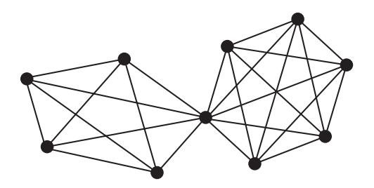
Figure 4. Kⁿ ⋆ K^m (n = 5, m = 6).

Let \(\tilde{D}\) be the distance matrix of \(\tilde{G} = K_n \star K_m\). It is convenient to write \(\tilde{D}\) in the block matrices:

\[\tilde{D} = \begin{bmatrix} J - I & S \\ \hline S^T & J - I \end{bmatrix}, \qquad S = \begin{bmatrix} 2 & \cdots & 2 \\ \vdots & & \vdots \\ 2 & \cdots & 2 \\ 1 & \cdots & 1 \end{bmatrix}, \tag{46}\]

where S is an \(n \times (m-1)\) matrix. The QE constant \(\mathrm{QEC}(\tilde{G})\) is the conditional maximum of

\[\Phi = \langle \tilde{f}, \tilde{D}\tilde{f} \rangle, \qquad \tilde{f} \in C(\tilde{V}), \tag{47}\]

subject to

\[\langle \tilde{f}, \tilde{f} \rangle = 1, \qquad \langle \mathbf{1}, \tilde{f} \rangle = 0.\]

According to the block diagonal expression (46), we write \(\tilde{f} = [f \ g]^T\), where \(f \in \mathbb{R}^n\), \(g \in \mathbb{R}^{m-1}\). Then (47) becomes

\[\Phi = \Phi(f, g) = \left\langle \begin{bmatrix} f \\ g \end{bmatrix}, \begin{bmatrix} J - I & S \\ S^T & J - I \end{bmatrix} \begin{bmatrix} f \\ g \end{bmatrix}, \right\rangle = \langle 1, f \rangle^2 + \langle 1, g \rangle^2 - \langle f, f \rangle - \langle g, g \rangle + 4\langle \mathbf{1}, f \rangle \langle \mathbf{1}, g \rangle - 2f_n \langle \mathbf{1}, g \rangle,\]

where we used

\[Sg = \langle \mathbf{1}, g \rangle [2 \ 2 \cdots \ 2 \ 1]^T.\]

Define

\[F(f, g, \lambda, \mu) = \Phi(f, g) - \lambda(\langle f, f \rangle + \langle g, g \rangle - 1) - \mu(\langle \mathbf{1}, f \rangle + \langle \mathbf{1}, g \rangle)\]

and let \(\mathcal{S}\) be the set of its stationary points \((f,g,\lambda,\mu)\in\mathbb{R}^n\times\mathbb{R}^{m-1}\times\mathbb{R}\times\mathbb{R}\), that is the solutions to

\[\frac{\partial F}{\partial f_i} = \frac{\partial F}{\partial g_j} = \frac{\partial F}{\partial \lambda} = \frac{\partial F}{\partial \mu} = 0, \quad 1 \le i \le n, \quad 1 \le j \le m - 1.\] (48)

Keeping in mind that \(-1 < \text{QEC}(\tilde{G}) < 0\) unless m = 1 or n = 1, we find after simple calculus that the maximum of \(\lambda\) appearing in the solution is

\[\lambda = \frac{-mn + \sqrt{mn(m-1)(n-1)}}{m+n-1} = -\frac{1}{1 + \sqrt{\left(1 - \frac{1}{m}\right)\left(1 - \frac{1}{n}\right)}},\]

which coincides with \(\mathrm{QEC}(\tilde{G})\) by the general theory mentioned in Subsection 2.2. We have thus obtained the following result.

Proposition 4.4. For \(m \ge 1\) and \(n \ge 1\) with \(m + n \ge 3\) with we have

\[QEC(K_n \star K_m) = -\frac{1}{1 + \sqrt{\left(1 - \frac{1}{m}\right)\left(1 - \frac{1}{n}\right)}}.\]

Corollary 4.2. We have

\[QEC(P_3) = QEC(K_2 \star K_2) < QEC(K_3 \star K_2) < \cdots\] \[\cdots < QEC(K_n \star K_2) < \cdots \rightarrow QEC(P_4) = -\frac{2}{2 + \sqrt{2}}.\] (49)

Proof. By Proposition 4.4 we have

QEC\[(K_n \star K_2) = -\frac{2}{2 + \sqrt{2(1 - \frac{1}{n})}}, \quad n \ge 1,\]

from which the assertion follows immediately.

Corollary 4.3. Let m ≥ 1 and n ≥ 1 with m + n ≥ 3. Then QEC(Kⁿ ⋆ Km) < QEC(P4) if and only if one of the following conditions is satisfied:

• (i) m = 2 and n ≥ 1;
• (ii) m ≥ 1 and n = 2;
• (iii) m = n = 3.

Proof. The inequality QEC(Kⁿ ⋆ Km) < QEC(P4) is equivalent to

\[-\frac{1}{1+\sqrt{\left(1-\frac{1}{m}\right)\left(1-\frac{1}{n}\right)}} < -\frac{2}{2+\sqrt{2}},\]

of which integer solutions are obtained easily by simple algebra.

Corollary 4.4. Let m ≥ 1 and n ≥ 1 with m + n ≥ 3. Then

\[QEC(P_3) \le QEC(K_n \star K_m) < QEC(P_4)\] (50)

holds if and only if one of the following conditions is satisfied:

• (i) m = 2 and n ≥ 2;
• (ii) m ≥ 2 and n = 2;
• (iii) m = n = 3.

The equality in (50) occurs only when m = n = 2.

4.4. Determining the class QEC(P3) ≤ QEC(G) < QEC(P4)

This subsection is devoted to the proof of the following result.

Theorem 4.2. A finite connected graph G fulfills the inequality

\[QEC(P_3) \le QEC(G) < QEC(P_4)\] (51)

if and only if G is a star product Kⁿ ⋆ K² with n ≥ 2 or K³ ⋆ K3. Moreover,

\[QEC(K_n \star K_2) = -\frac{2}{2 + \sqrt{2\left(1 - \frac{1}{n}\right)}},\]\[QEC(K_3 \star K_3) = -\frac{3}{5}.\]

In particular, QEC(G) = QEC(P3) if and only if G = P³ = K² ⋆ K2.

Lemma 4.1. If a connected graph G = (V, E) satisfies (51), we have |V | ≥ 3 and diam(G) = 2.

Proof. It follows from Corollary 2.2 that diam(G) ≤ 2. If diam(G) = 1, then G is a complete graph and QEC(G) = −1, which does not satisfy (51). Hence, necessarily diam(G) = 2 and |V | ≥ 3.

In general, a clique of G is an induced subgraph of G which is isomorphic to a complete graph. A clique K = (W, F) is called maximal if there is no clique containing K properly. A maximal clique K = (W, F) is called largest or maximum if there is no clique on |W| + 1 vertices. Clearly, any graph contains a largest clique.

Lemma 4.2. Let G = (V, E) be a connected graph satisfying (51). If K = (W, F) is a maximal clique of G, we have W ̸= V and |W| ≥ 2.

Proof. Since G is not a complete graph by Lemma 4.1, we have W ̸= V . That |W| ≥ 2 follows from |V | ≥ 3.

Lemma 4.3. Let G = (V, E) be a connected graph with |V | ≥ 2 and QEC(G) < −1/2, and K = (W, F) a maximal clique. Then for any pair a ∈ V \W and a ′ ∈ W with a ∼ a ′ we have {x ∈ W ; x ∼ a} = {a ′}.

Proof. (Note that the assertion is trivial if W = V .) Given a pair a ∈ V \W and a ′ ∈ W with a ∼ a ′ , we set s = |{x ∈ W ; x ∼ a}|. Obviously, 1 ≤ s < |W|. We will show by contradiction that s = 1. Suppose that s ≥ 2. Then there exist three distinct vertices x1, x2, y ∈ W such that a ∼ x1, a ∼ x² and a ̸∼ y. Note that the induced subgraph spanned by {a, x1, x2, y} is isomorphic to a diamond K4\{e}. It then follows immediately from Proposition 4.2 that QEC(G) ≥ −1/2, which is in contradiction to the assumption QEC(G) < −1/2.

Lemma 4.4. Let G = (V, E) be a connected graph satisfying (51) and K = (W, F) a maximal clique of G. For a, b ∈ V \W and a ′ , b′ ∈ W, if a ∼ a ′ and b ∼ b ′ , then a ′ = b ′ .

Proof. If a = b the assertion follows immediately from Lemma 4.3. We consider the case of a ̸= b. To prove the assertion by contradiction, we assume that a ′ ̸= b ′ . Since d(a, b) ≤ diam(G) = 2, we have two cases: d(a, b) = 1 or d(a, b) = 2.

Suppose first that d(a, b) = 1, that is, a ∼ b. Then the induced subgraph spanned by {a, a′ , b′ , b} is isomorphic to C4, which is a forbidded subgraph by Corollary 4.1. Hence d(a, b) = 1 does not happen.

Suppose next that d(a, b) = 2. Then there exists c ∈ V such that a ∼ c ∼ b. Since a ̸∼ b ′ and b ̸∼ a ′ by Lemma 4.3, we have c ̸= a ′ , b′ and c ̸∈ W. There are four cases:

• (i) c ̸∼ a ′ and c ̸∼ b ′ . The induced subgraph spanned by {a, a′ , b′ , b, c} is isomorphic to C5, which is a forbidded subgraph by Corollary 4.1.
• (ii) c ̸∼ a ′ and c ∼ b ′ . The induced subgraph spanned by {a, a′ , b′ , c} is isomorphic to C4, which is a forbidded subgraph by Corollary 4.1.
  • (iii) c ∼ a ′ and c ̸∼ b ′ . This case is similar to (ii).
• (iv) c ∼ a ′ and c ∼ b ′ . This does not happen by virtue of Lemma 4.3. In any case we come to contradiction and the proof is completed.

Proof of Theorem 4.2. Let G = (V, E) be a connected graph satisfying (51) K = (W, F) be a largest clique with m = |W|. Note that V ̸= W and m ≥ 2 by Lemma 4.2. Now divide V \W into two subsets:

\[V\backslash W=U_1\cup U_2\,,\]

where U¹ is the set of vertices a ∈ V \W which are directly connected to vertices in W, and U² the rest, see Figure 5. Obviously, U¹ ̸= ∅. Moreover, by Lemma 4.4 there exists a unique a ′ ∈ W such that a ∼ a ′ for all a ∈ U1.

We first prove that U² = ∅. Suppose otherwise. Take x ∈ W with x ̸= a ′ and y ∈ U2. Then we have d(x, y) ≥ 3, which is in contradiction to diam(G) = 2.

We next prove that any pair of vertices a, b ∈ U1, a ̸= b, are connected by an edge. Suppose otherwise. Take x ∈ W with x ̸= a ′ and consider the induced subgraph spanned by {x, a′ , a, b} is isomorphic to K1,3, which is a forbidded subgraph by Corollary 4.1.

Consequently, The induced subgraph spanned by U¹ is a complete graph on |U1| ≥ 1 vertices. Hence G is necessarily a star product of two complete graphs: G = K^m ⋆ K|U1|+1. Then the assertion follows from Corollary 4.4.

Figure 5. V = W ∪ U¹ ∪ U2.

4.5. Bearded Complete Graphs \(BK_{n,m}\)

We are also interested in characterization of a graph G satisfying

\[QEC(G) = QEC(P_4) = -\frac{2}{2 + \sqrt{2}}.\]

Below we give a partial answer.

Let \(1 \le m \le n\). Consider a graph on

\[V = \{1, 2, \dots, n\} \cup \{n + 1, \dots, n + m\}\]

with edge set

\[E = \{\{i, j\}; 1 \le i < j \le n\} \cup \{\{i, n + i\}; 1 \le i \le m\}.\]

The induced subgraph spanned by \(\{1, 2, ..., n\}\) is the complete graph \(K_n\). We write \(G = BK_{n,m}\) and call it a bearded complete graph.

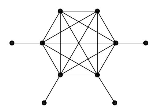
Figure 6. \(BK_{n,m}\) (n = 6, m = 4).

The distance matrix D of \(G = BK_{n,m}\) is written in the block matrices:

\[D = \begin{bmatrix} J - I & J & 2J - I \\ J & J - I & 2J \\ \hline 2J - I & 2J & 3J - 3I \end{bmatrix},\] (52)

where the diagonal matrices are of \(m \times m\), \((n-m) \times (n-m)\) and \(m \times m\), in order.

For m = n = 1 by definition \(BK_{1,1} = K_2\). Hence

\[QEC(BK_{1,1}) = -1.\]

For m = 1 and n ≥ 2 we have BKn,¹ = Kⁿ ⋆ K² = Kⁿ ∧ K1,1. It is already known that

QEC\[(BK_{n,1}) = -\frac{2}{2 + \sqrt{2(1 - \frac{1}{n})}}\].

The above formula is valid for n = 1.

Theorem 4.3. Let 2 ≤ m ≤ n. Then

\[QEC(BK_{n,m}) = -\frac{2}{2+\sqrt{2}} = -(2-\sqrt{2}) = QEC(P_4).\]

Proof. According to the expression (52) in block diagonal form, the quadratic function Φ = ⟨ ˜f, D ˜f⟩ becomes

\[\Phi = \left\langle \begin{bmatrix} f \\ g \\ h \end{bmatrix}, \begin{bmatrix} J - I & J & 2J - I \\ J & J - I & 2J \\ 2J - I & 2J & 3J - 3I \end{bmatrix}, \begin{bmatrix} f \\ g \\ h \end{bmatrix} \right\rangle = \left\langle \mathbf{1}, f \right\rangle^2 + \left\langle \mathbf{1}, g \right\rangle^2 + 3\left\langle \mathbf{1}, h \right\rangle^2 - \left\langle f, f \right\rangle - \left\langle g, g \right\rangle - 3\left\langle h, h \right\rangle + 2\left\langle \mathbf{1}, f \right\rangle \left\langle \mathbf{1}, g \right\rangle + 4\left\langle \mathbf{1}, f \right\rangle \left\langle \mathbf{1}, h \right\rangle + 4\left\langle \mathbf{1}, g \right\rangle \left\langle \mathbf{1}, h \right\rangle - 2\left\langle f, h \right\rangle,\]

where

\[\tilde{f} = \begin{bmatrix} f \\ g \\ h \end{bmatrix}, \qquad f \in \mathbb{R}^m, \quad g \in \mathbb{R}^{n-m}, \quad h \in \mathbb{R}^m.\]

We then consider the stationary points of

\[F(f, g, h, \lambda, \mu) = \Phi - \lambda(\langle f, f \rangle + \langle g, g \rangle + \langle h, h \rangle - 1) - \mu(\langle \mathbf{1}, f \rangle + \langle \mathbf{1}, g \rangle + \langle \mathbf{1}, h \rangle).\]

After simple calculus we see that the largest λ appearing in the stationary points of F(f, g, h, λ, µ) is given by √

\[\lambda = -(2 - \sqrt{2}),\]

with

\[\langle \mathbf{1}, f \rangle = 0, \quad \langle f, f \rangle = \frac{2 + \sqrt{2}}{4}, \quad g = 0, \quad h = -(\lambda + 1)f, \quad \mu = 0.\]

Indeed, by virtue of the condition m ≥ 2, we may choose f ∈ R ^m satisfying the first two conditions.

Note

The QE constants of graphs on n vertices with n ≤ 5 are listed in [18], in which the QE constant of the graph No. 12 on n = 5 verices needs correction:

for \[-\frac{4}{5+\sqrt{5}}\] read \(-\frac{4}{5+\sqrt{15}}\)

Acknowledgement

The second author thanks Institut Teknologi Bandung for their kind hospitality, where this work was completed in March 2019. The support by JSPS Open Partnership Joint Research Project "Extremal graph theory, algebraic graph theory and mathematical approach to network science" (2017–18) is gratefully acknowledged. He also thanks Professor J. Koolen for a stimulating discussion.

References

• [1] G. Aalipour, A. Aida, Z. Berikkyzy, J. Cummings, and J. De Silva, On the distance spectra of graphs, Linear Algebra Appl. 497 (2016), 66–87.
• [2] M. Aouchiche and P. Hansen, Distance spectra of graphs: a survey, Linear Algebra Appl. 458 (2014), 301–386.
• [3] R. Balaji and R.B. Bapat, On Euclidean distance matrices, Linear Algebra Appl. 424 (2007), 108–117.
• [4] M. Bozejko, T. Januszkiewicz, and R.J. Spatzier, Infinite Coxeter groups do not have Kazh- ˙ dan's property, J. Operator Theory 19 (1988), 63–67.
• [5] M. Bozejko, Positive-definite kernels, length functions on groups and noncommutative von ˙ Neumann inequality, Studia Math. 95 (1989), 107–118.
• [6] M.M. Deza and M. Laurent, Geometry of Cuts and Metrics, Springer-Verlag, Berlin, 1997.
• [7] R. Faudree, E. Flandrin, and Z. Ryja´cek, Claw-free graphs A survey, ˇ Discrete Math. 164 (1997), 87–147.
• [8] U. Haagerup, An example of a nonnuclear C^∗ -algebra which has the metric approximation property, Invent. Math. 50 (1979), 279–293.
• [9] G. Indulal and I. Gutman, On the distance spectra of some graphs, Mathematical Communications 13 (2008), 123–131.
• [10] G. Jaklic and J. Modic, On Euclidean distance matrices of graphs, ˇ Electron. J. Linear Algebra 26 (2013), 574–589.
• [11] G. Jaklic and J. Modic, Euclidean graph distance matrices of generalizations of the star graph, ˇ Appl. Math. Comput. 230 (2014), 650–663.
• [12] J. H. Koolen and S. V. Shpectorov, Distance-regular graphs the distance matrix of which has only one positive eigenvalue, European J. Combin. 15 (1994), 269–275.
• [13] L. Liberti, G. Lavor, N. Maculan, and A. Mucherino, Euclidean distance geometry and applications, SIAM Rev. 56 (2014), 3–69.

• [14] W. Młotkowski and N. Obata, On quadratic embedding constants of star product graphs, Hokkaido Math. J. 49 (2020), 129–163.
• [15] N. Obata, Positive Q-matrices of graphs, Studia Math. 179 (2007), 81–97.
• [16] N. Obata, Markov product of positive definite kernels and applications to Q-matrices of graph products, Colloq. Math. 122 (2011), 177–184.
• [17] N. Obata, Quadratic embedding constants of wheel graphs, Interdiscip. Inform. Sci. 23 (2017), 171–174.
• [18] N. Obata and A.Y. Zakiyyah, Distance matrices and quadratic embedding of graphs, Electron. J. Graph Theory Appl. 6 (1) (2018), 37–60.
• [19] I.J. Schoenberg, Remarks to Maurice Frechet's article "Sur la d ´ efinition axiomatique d'une ´ classe d'espace distancis vectoriellement applicable sur l'espace de Hilbert", Ann. Math. ´ 36 (1935), 724–732.
• [20] I.J. Schoenberg, Metric spaces and positive definite functions, Trans. Amer. Math. Soc. 44 (1938), 522–536.