Suzana Antunovic´ a , Damir Vukicevi ˇ c´ b
santunovic@gradst.hr, vukicevic@pmfst.hr
Directed acyclic graphs are often used to model situations and problems in real life. If we consider the topological ordering of a graph as a process of arranging the vertices in the best possible way considering the constraints caused by the direction of edges, then it makes sense to try to optimize this process by minimizing the distances between vertices in the ordering. For this purpose, we define measures based on distances between vertices in the topological ordering that allow us to construct a graph with optimal topological ordering regarding a specific measure thus minimizing the complexity of the system represented by the graph. We explore minimal and maximal values of the defined measures and comment on the topology of graphs for which maximal and minimal values are obtained. Potentially, the proved bounds could be used to benchmark existing algorithms, devise new approximation algorithms or branch–and–bound schemas for some scheduling problems that are usually of hard computational complexity.
Keywords: directed acyclic graph, topological order, measure, extremal values Mathematics Subject Classification : 05C20, 05C35, 05C12, 94C15
DOI: 10.5614/ejgta.2021.9.2.25
1. Introduction
Graphs are used to model many situations and problems that arise in different areas of interest. Special class of graphs that occur widely in natural and man-made settings are directed acyclic graphs [14]. The term refers to a finite directed graph that has no directed cycles. In computer
Received: 15 September 2020, Revised: 13 July 2021, Accepted: 3 October 2021.
aFaculty of Civil Engineering, Architecture and Geodesy, University of Split, Croatia
bFaculty of Science, University of Split, Croatia
science and engineering acyclic graphs occur in data structures, software call graphs, feed-forward neural networks and parallel processing. In pure mathematics acyclic graphs are studied for their own sake [4, 17], as a representation of partially ordered sets [20] and random graph orders [1, 7], while in statistics the widely used Bayesian networks are an acyclic graph version of probabilistic graphical models [12, 13, 16].
Every directed acyclic graph has a topological ordering [3], a linear ordering of its vertices in such way that for every directed edge the starting vertex of the edge occurs earlier in the sequence than the ending vertex of the edge. For instance, the vertices of the graph may represent tasks to be performed, and the edges may represent constraints that one task must be performed before another. If we consider topological ordering as a process of arranging the vertices in the best possible way considering the constraints caused by the direction of edges, then it makes sense to try to optimize it by minimizing the distances between vertices in the ordering. This allows for a process that is represented by a directed acyclic graph to be more efficient (whether in execution time or in minimizing any cost function defined on the graph). This problem is widely researched in computer science, especially in parallel processing. It is known as task scheduling problem and the research resulted in many algorithms in an effort to find the optimal solution [5, 9, 10, 19]. There has been a lot of work done to form a mathematical background for researching this problem [8, 11, 15]. In mathematics, this problem is referred to as a linear ordering problem [6], [18].
In this paper we define new measures for evaluating the topological ordering of vertices in directed acyclic graphs. Measures were motivated by curriculum networks presented in [2], where vertices represent education units and directed edge uv denotes that unit u is a necessary prerequisite for unit v. Using these measures one can construct a curriculum in such a way that minimal time is needed for the student to master the materials. We define measures for single vertex, which incorporate how a vertex depends on its incoming neighbours. We then generalize the measures for entire graph and bound their values over a set of all topological orderings of given dag. Finally, we give an example of a graph for which the minimal and maximal value of a certain measure is obtained. Two types of families of graphs were considered: weakly connected directed acyclic graphs and weakly connected directed acyclic graphs that are transitively closed. Note that we give one possible graph for which equality holds, we do not claim that this graph is a unique solution.
2. Mathematical framework
Let G = (V, E) be a directed acyclic graph and let P(G) be the set of all bijections p : V (G) → {1, . . . , n} such that it holds that p(u) < p(v) for each directed edge uv ∈ E(G). We can consider P(G) to be the set of all topological orderings of a directed acyclic graph. Let us denote dp(uv) = p(v) − p(u) for each directed edge uv ∈ E(G), which is actually the distance between vertices u and v in the topological ordering p. Using these distances, we can define new measures for vertices in directed acyclic graphs. For each vertex v ∈ V (G), we define sp,G(v) as the sum of distances between v and every of its incoming neighbours,
\[s_{p,G}(v) = \sum_{uv \in E(G)} d_p(uv).\]
We can interpret this measure as a cost that vertex makes to the network or as the amount of time needed for all of the immediate prerequisites of vertex v to be completed. We can also consider the average distance between v and its incoming neighbours resulting in measure \(a_{p,G}(v)\) and the maximal distance between v and its incoming neighbours resulting in measure \(m_{p,G}(v)\),
\[a_{p,G}(v) = \begin{cases} \frac{s_{p,G}(v)}{d_G^-(v)}, & \text{if } d_G^-(v) > 0, \\ 0, & \text{if } d_G^-(v) = 0, \end{cases}\]\[m_{p,G}(v) = \max_{uv \in E(G)} \left\{ d_p(uv) \right\},\]
where \(d_G^-(v)\) denotes in-degree of a vertex \(v \in V(G)\). Another way to interpret these measures is in terms of complexity for a single vertex: \(s_{p,G}(v)\) states that a vertex is as complex as the sum of complexities of all of its immediate prerequisites, \(a_{p,G}(v)\) and \(m_{p,G}(v)\) take into account the average and maximal complexity of its immediate prerequisites respectively.
We now expend these measures to the entire directed acyclic graph G with n vertices. There are number of ways to approach this problem. The simplest way is to sum through all the vertices and divide by the number of vertices, which gives us the following measures:
\[s_p^1(G) = \frac{1}{n} \sum_{v \in V(G)} s_{p,G}(v),\] \[a_p^1(G) = \frac{1}{n} \sum_{v \in V(G)} a_{p,G}(v),\] \[m_p^1(G) = \frac{1}{n} \sum_{v \in V(G)} m_{p,G}(v).\]
We can also consider finding maximal values over all vertices in the graph.
\[s_p^{\infty}(G) = \max_{v \in V(G)} \{ s_{p,G}(v) \},\] \[a_p^{\infty}(G) = \max_{v \in V(G)} \{ a_{p,G}(v) \},\] \[m_p^{\infty}(G) = \max_{v \in V(G)} \{ m_{p,G}(v) \}.\]
One can also consider the \(\alpha\)-mean values between these two cases:
\[s_p^\alpha(G) = \left(\frac{1}{n} \sum_{v \in V(G)} s_{p,G}^\alpha(v)\right)^{\frac{1}{\alpha}},\]
\[a_p^{\alpha}(G) = \left(\frac{1}{n} \sum_{v \in V(G)} a_{p,G}^{\alpha}(v)\right)^{\frac{1}{\alpha}},\]
\[m_p^{\alpha}(G) = \left(\frac{1}{n} \sum_{v \in V(G)} m_{p,G}^{\alpha}(v)\right)^{\frac{1}{\alpha}}.\]
Since the topological ordering od directed acyclic graph is generally not unique, we define
\[s^{\alpha}(G) = \min_{p \in P(G)} \left\{ s_p^{\alpha}(G) \right\},\,\]
\[a^{\alpha}(G) = \min_{p \in P(G)} \left\{ a_p^{\alpha}(G) \right\},\,\]
\[m^{\alpha}(G) = \min_{p \in P(G)} \left\{ m_p^{\alpha}(G) \right\}.\]
and are interested in finding upper and lower bound for these values for α ≥ 1. We shall study two types of families of graphs:
- 1. Type A weakly connected directed acyclic graphs.
- 2. Type B weakly connected directed acyclic graphs that are transitively closed.
A graph G is weakly connected if its underlying undirected graph (all edges replaced by undirected edges) is connected. Graph G is transitively closed if there is an edge uv ∈ E(G) corresponding to each directed path from u to v in G.
3. Extremal results
Figure 1: Simple examples of graphs for n = 5: (a) G = Sn (b) G = Tn (c) G = On (d), (e) Disoriented path
Let n be the number of vertices in a graph G. Let us denote G = Sn a directed graph which underlying graph is a star and all edges are oriented from the center of the star toward a pendant vertex (see Figure 1 (a)). Let G = On be a directed graph that corresponds to total linear order of n elements (equivalently, let On be simple directed graph without directed cycles which underlying graph is complete graph or equivalently let On be a tournament without directed cycles). Example
of O5 is given in Figure 1 (c). Let G = Pn be a directed path, i.e. digraph with n vertices which underlying graph is a path and for each i it holds ei = (vi−1, vi). Disoriented path on n vertices is a directed graph with n vertices which underlying graph is a path, but there are no directed paths such that d(u, v) ≥ 2 (see Figure 1 (d) and (e)). In this case d(u, v) represents standard graph–theoretical distance between vertices u and v. Note that there are (up to isomorphism) two disoriented paths for odd n and only one for even n.
3.1. Graphs of type A
Theorem 3.1. Let G be a directed graph of type A with n ≥ 3 vertices. It holds
- 1. 1 ≤ m∞(G) ≤ n − 1. The lower bound is obtained for G = Pn and the upper bound is obtained for G = On.
- 2. 1 ≤ s ∞(G) ≤ nP−1 i=1 i. The lower bound is obtained for G = Pn and the upper bound is obtained for G = On.
- 3. 1 ≤ a ∞(G) ≤ n − 1. The lower bound is obtained for G = Pn and the upper bound is obtained for G = Sn.
Proof. By definition, for graph G it holds p(u) < p(v) for each uv ∈ E(G) for each permutation p, so p(v)−p(u) > 0. Since bijection p is defined with p : V (G) → {1, . . . , n} it holds p(v)−p(u) < n. From this we conclude that 1 ≤ m∞(G) ≤ n − 1. It can easily be calculated that the lower bound is obtained for Pn and the upper for On. This proves 1. The other claims are trivial.
Theorem 3.2. Let G be a directed graph of type A with n ≥ 3 vertices and α ≥ 1. It holds
\[\left(\frac{n-1}{n}\right)^{\frac{1}{\alpha}} \le m^{\alpha}(G) \le \left(\frac{1}{n}\sum_{i=1}^{n-1}i^{\alpha}\right)^{\frac{1}{\alpha}}.\]
The lower bound is obtained for G = Pn and the upper bound for G = On.
Proof. Let G be a directed graph with n ≥ 3 vertices and let p be a bijection that minimizes mα (G). Let us note that graph G has at least n − 1 arcs since it is weakly connected. It holds
\[m_p^{\alpha}(G) = \left[\frac{1}{n} \sum_{v \in V(G)} m_{p,G}^{\alpha}(v)\right]^{\frac{1}{\alpha}} \ge \left[\frac{1}{n} \sum_{v \in V(G)} (d_G^-(v))^{\alpha}\right]^{\frac{1}{\alpha}}.\]
Note that x α is a convex function for α > 1 and that at least one in-degree is equal to 0, hence:
\[\begin{split} & \left[\frac{1}{n}\sum_{v\in V(G)}(d_G^-(v))^{\alpha}\right]^{\frac{1}{\alpha}} \geq \left[\frac{(n-1)}{n}\left(\frac{\sum\limits_{v\in V(G)}d_G^-(v)}{n-1}\right)^{\alpha}\right]^{\frac{1}{\alpha}} \geq \\ & \geq \left[\frac{(n-1)}{n}\left(\frac{e(G)}{n-1}\right)^{\alpha}\right]^{\frac{1}{\alpha}} \geq \left[\frac{(n-1)}{n}\left(\frac{n-1}{n-1}\right)^{\alpha}\right]^{\frac{1}{\alpha}} = \left(\frac{n-1}{n}\right)^{\frac{1}{\alpha}}, \end{split}\]
where e(G) denotes the number of directed edges in graph G. The upper bound follows because for every two vertices \(u, v \in V(G)\) it holds \(p(v) - p(u) \le p(v) - 1\), which is true if vertex u such that p(u) = 1 points to all other vertices.
Theorem 3.3. Let G be a directed graph of type A with \(n \geq 3\) vertices and \(\alpha \geq 1\). It holds
\[\left(\frac{n-1}{n}\right)^{\frac{1}{\alpha}} \le s^{\alpha}(G) \le \left[\frac{1}{n} \sum_{i=2}^{n} \left(\sum_{j=1}^{i-1} j\right)^{\alpha}\right]^{\frac{1}{\alpha}}.\]
The lower bound is obtained for \(G = P_n\) and the upper bound for \(G = O_n\).
Proof. The lower bound follows from Theorem 3.2. The upper bound is trivial since the value of \(s_{p,G}^{\alpha}(v)\) will be highest if all the edges that can point to a vertex \(v \in V(G)\) really do point to it. \(\square\)
Let us denote \(T_{n,k}\) a graph obtained from graph \(P_k\) by adding the remaining n-k vertices in such a way that all arcs point to vertices on \(P_k\) and every vertex in \(P_k\) has equal in-degree. The example of such graph is shown on Fig. 2.
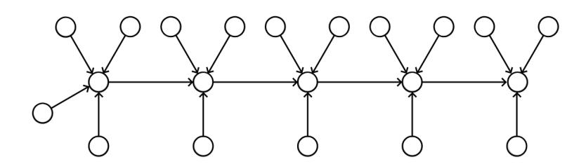
Figure 2: Example of graph \(G = T_{n,k}\) for k = 5 and n = 21
Theorem 3.4. Let G be a directed graph of type A with \(n \geq 3\) vertices and \(\alpha \geq 1\). It holds
\[a^{\alpha}(G) \geq \begin{cases} \frac{n}{2n^{\frac{1}{\alpha}}}, & \text{if } \alpha \leq \frac{1}{n-1} + 1, \\ \frac{\alpha}{2(\alpha - 1)} \left[ \frac{1}{n}(n - 1)(\alpha - 1) \right]^{\frac{1}{\alpha}}, & \text{if } \frac{1}{n-1} + 1 < \alpha < 2, \\ \left( \frac{n-1}{n} \right)^{\frac{1}{\alpha}}, & \text{if } \alpha \geq 2. \end{cases}\]
The lower bound is obtained for \(G=T_n\) if \(\alpha \leq 1/(n-1)+1\), for \(G=T_{n,k}\) where \(k=(n-1)(\alpha-1)\) and \(1/(n-1)+1<\alpha<2\) or for \(G=P_n\) if \(\alpha \geq 2\).
Proof. Let G be a directed graph with \(n \geq 3\) vertices and let p be a bijection that minimizes \(a^{\alpha}(G)\). Graph G has at least n-1 arcs. It holds
\[a_p^{\alpha}(G) = \left[\frac{1}{n} \sum_{v \in V(G)} a_{p,G}^{\alpha}(v)\right]^{\frac{1}{\alpha}} \ge \left[\frac{1}{n} \sum_{\substack{v \in V(G) \\ d_G^-(v) \neq 0}} \left(\frac{\sum_{i=1}^{d_G^-(v)} i}{d_G^-(v)}\right)^{\alpha}\right]^{\frac{1}{\alpha}} \ge \left[\frac{1}{n} \sum_{\substack{v \in V(G) \\ d_G^-(v) \neq 0}} \left(\frac{d_G^-(v) + 1}{2}\right)^{\alpha}\right]^{\frac{1}{\alpha}}.\]
Let x ∈ {1, . . . , n − 1} be the number of vertices v such that d − G(v) 6= 0. It holds:
\[a_p^{\alpha}(G) \ge \left[\frac{x}{n} \left(\frac{e(G) + x}{2x}\right)^{\alpha}\right]^{\frac{1}{\alpha}} \ge \left[\frac{x}{2^{\alpha}n} \left(\frac{n - 1 + x}{x}\right)^{\alpha}\right]^{\frac{1}{\alpha}}.\]
We need to minimize the function
\[f(x) = x \left(\frac{n-1+x}{x}\right)^{\alpha}\].
First derivation gives us that function has minimum for x = (n − 1)(α − 1). Since it holds that x ∈ {1, . . . , n − 1}, we get the following cases:
- 1. If (n − 1)(α − 1) ≤ 1 then a α (G) will have its minimal value for x = 1
- 2. If 1 < (n − 1)(α − 1) < n − 1 then a α (G) will have its minimal value if x and 1/(α − 1) are integers and x | (n − 1)
- 3. If (n − 1)(α − 1) ≥ n − 1 then a α (G) will have its minimal value for x = n − 1.
Lower bounds can easily be calculated from this.
Theorem 3.5. Let G be a directed graph of type A with n ≥ 3 vertices and α ≥ 1. It holds
\[a^{\alpha}(G) \le \left(\frac{1}{n} \sum_{i=1}^{n-1} i^{\alpha}\right)^{\frac{1}{\alpha}}.\]
The upper bound is obtained for G = Sn.
Proof. Trivial.
The results obtained for graphs of type A are summerized in Table 1.
Table 1: Extremal values for the graphs of type A
| Measure | Minimal | Maximal |
|---|---|---|
| ∞(G) s | 1 | nP−1 i i=1 |
| ∞(G) a | 1 | − n 1 |
| m∞(G) | 1 | n − 1 |
| α s (G) | 1 n−1 α n | !α# 1 " α Pn i −1 1 P j n i=2 j=1 |
| α a (G) | i 1 1 h (n−1)(α−1) α n α n−1 min , , α 1 2(α−1) n n 2n α | 1 nP−1 α 1 α i n i=1 |
| mα (G) | 1 n−1 α n | 1 nP−1 α 1 α i n i=1 |
3.2. Graphs of type B
Let us now consider graphs of type B. Graph of type B is a weakly connected directed graph that does not contain directed cycles and that is transitively closed. Using Theorems 3.1 through 3.5 we get the following corollary.
Corollary 3.1. Let G be a directed graph of type B with n ≥ 3 vertices and α ≥ 1. It holds:
- 1. m∞(G) ≤ n − 1. The upper bound is obtained for G = On.
- 2. s ∞(G) ≤ nP−1 i=1 i. The upper bound is obtained for G = On.
- 3. a ∞(G) ≤ n − 1. The upper bound is obtained for G = Sn.
- 4. mα (G) ≤ 1 n nP−1 i=1 i α 1 α . The upper bound is obtained for G = On.
- 5. s α (G) ≤ 1 n Pn i=2 i P−1 j=1 j !α!1 α . The upper bound is obtained for G = On.
- 6. a α (G) ≤ n nP−1 i=1 i α 1 α . The upper bound is obtained for G = Sn.
Let us define by UT(G) a graph obtained by successive elimination of transitive edges, i.e. by the following algorithm:
- 1. Let G1 = G, i = 1, proceed=true
- 2. While proceed
- 2.1. If there are vertices u1, u2, . . . , uk ∈ V (G1) such that u1u2, u2u3, . . . , uk−1uk ∈ E(Gi) and u1uk ∈ E(Gi) then
2.1.1. \[G_{i+1} = G_i - u_1 u_k\] and \(i = i + 1\)
- 2.2. Else
- 2.2.1. proceed=false
- 3. UT(G) = Gi
Note that if graph G is weakly connected, then graph UT(G) is also weakly connected. Also, if graph G is strongly connected, then graph UT(G) is also strongly connected. Let ut(G) be underlying (unoriented) graph of graph UT(G). Note that UT(G) is connected.
Theorem 3.6. Let G be a directed graph of type B with \(n \ge 2\) vertices. It holds
\[\frac{2n-3}{n} \le s^1(G).\]
The lower bound is obtained for disoriented path.
Proof. We prove the claim by induction on n. For n=2, the claim is obvious. Now suppose that we have proved the claim for all graphs with n-1 vertices, \(n\geq 3\), and let G have n vertices. Let vertex u be a non-cut vertex of graph UT(G) (i.e. such vertex that UT(G)-u is weakly connected). From the induction hypothesis it follows that \(s^1(G-u)\geq \frac{2n-5}{n-1}\). If \(d^+_G(u)+d^-_G(u)\geq 2\), then there are at least two new arcs in G when compared to G-u. Let G be the permutation that minimizes \(s^1_p(G)\) and G permutation that minimizes \(g^1_p(G)\) and G permutation that minimizes \(g^1_p(G)\) and G permutation that minimizes \(g^1_p(G)\) and G permutation that minimizes \(g^1_p(G)\) and G permutation that minimizes \(g^1_p(G)\) and G permutation that minimizes \(g^1_p(G)\) and G permutation that minimizes \(g^1_p(G)\) and G permutation that minimizes \(g^1_p(G)\) and G permutation that minimizes \(g^1_p(G)\) and G permutation that minimizes \(g^1_p(G)\) and G permutation that minimizes \(g^1_p(G)\) and G permutation that minimizes \(g^1_p(G)\) and G permutation that minimizes \(g^1_p(G)\) and G permutation that minimizes \(g^1_p(G)\) and G permutation that minimizes \(g^1_p(G)\) and G permutation that minimizes \(g^1_p(G)\) and G permutation that minimizes \(g^1_p(G)\) and G permutation that minimizes \(g^1_p(G)\) and G permutation that minimizes \(g^1_p(G)\) and G permutation that minimizes \(g^1_p(G)\) and G permutation that minimizes \(g^1_p(G)\) and G permutation that minimizes \(g^1_p(G)\) and G permutation that minimizes \(g^1_p(G)\) and G permutation that minimizes \(g^1_p(G)\) and G permutation that minimizes \(g^1_p(G)\) and G permutation that G permutation that G permutation that G permutation that G permutation that G permutation that G permutation that G permutation that G permutation that G permutation that G permutation that G permutation that G permutation that G permutation that G permutation that G permutation that G permutation that G perm
\[s^{1}(G) = s_{q}^{1}(G) \ge \frac{2 + (n-1)s_{q/(V(G)-u)}^{1}(G-u)}{n} \ge \frac{2 + (n-1)s_{r}^{1}(G-u)}{n} \ge \frac{2 + (2n-5)}{n} = \frac{2n-3}{n}.\]
Hence, \(d_G^+(u)+d_G^-(u)=1\). Let us distinguish two cases: \(uv\in E(G)\) and \(vu\in E(G)\). We shall prove the theorem for \(uv\in E(G)\), the other case is analogous. If \(uv\in E(G)\) it follows that there is a vertex w such that \(wv\in E(UT(G))\). Let q be a permutation that minimizes \(s_q^1(G)\). If \(q(v)-q(u)\geq 2\), then it holds
\[s_q^1(G) \ge \frac{[q(v) - q(u)] + (n-1) \cdot s_{q/V(G) - u}^1(G)}{n} \ge 2 + (n-1) \cdot s^1(G)\]\[\ge \frac{2 + 2n - 5}{n} = \frac{2n - 3}{n}.\]
If q(v) - q(u) = 1 then let us denote \(r: V(G) \to \bullet\) function defined by:
\[r(x) = \begin{cases} q(x), & \text{if } q(x) < q(u), \\ q(x) - 1, & \text{if } q(x) > q(u). \end{cases}\]
Note that for every edge \(x_1x_2 \in E(G)\) it holds \(r(x_2)-r(x_1) \leq q(x_2)-q(x_1)\) and that \(r(v)-r(w) \leq q(v)-q(w)-1\). Hence,
\[\begin{split} s_q^1(G) & \geq \frac{\left[q(v) - q(u)\right] + (n-1) \cdot s_{q/G - u}^1(G)}{n} \geq \frac{1 + (n-1) \cdot \left(s_r^1(G) + \frac{1}{n-1}\right)}{n} \\ & \geq \frac{1 + (n-1) \cdot \left(s^1(G) + \frac{1}{n-1}\right)}{n} \geq \frac{1 + (n-1) \cdot \left(\frac{2n-5}{n-1} + \frac{1}{n-1}\right)}{n} = \frac{2n-3}{n}. \end{split}\]
This proves the inequality. It is simple to check that equality holds for disoriented path. \(\Box\)
Theorem 3.7. Let G be a directed graph of type B with \(n \ge 5\) vertices. It holds
\[\frac{n-1}{n} \le m^1(G).\]
The lower bound is obtained for \(G = T_n\).
Proof. Let G be a directed graph of type B with n ≥ 5 vertices and let p be a bijection that minimizes m1 p (G). Graph G has at least n − 1 arcs. It holds:
\[m_p^1(G) = \frac{1}{n} \sum_{v \in V(G)} m_{p,G}(v) \ge \frac{1}{n} \sum_{v \in V(G)} d_G^-(v) \ge \frac{e(G)}{n} \ge \frac{n-1}{n}.\]
Theorem 3.8. Let G be a directed graph of type B with n ≥ 5 vertices. It holds 1 2 ≤ a 1 (G). The lower bound is obtained for G = Tn.
Proof. Let G be a directed graph of type B with n ≥ 5 vertices and let p be a bijection that minimizes a 1 p (G). Graph G has at least n − 1 arcs. It holds:
\[a_p^1(G) = \frac{1}{n} \sum_{v \in V(G)} a_{p,G}(v) \ge \frac{1}{n} \sum_{\substack{v \in V(G) \\ d_G^-(v) \ne 0}} \left( \frac{\sum_{i=1}^{d_G^-(v)} i}{d_G^-(v)} \right) \ge \frac{1}{n} \sum_{\substack{v \in V(G) \\ d_G^-(v) \ne 0}} \left( \frac{d_G^-(v) + 1}{2} \right).\]
Let x ∈ {1, . . . , n − 1} be the number of vertices v such that d − G(v) 6= 0. It holds:
\[\frac{1}{n} \sum_{\substack{v \in V(G) \\ d^-_G(v) \neq 0}} \left( \frac{d^-_G(v) + 1}{2} \right) \geq \frac{n - 1 + x}{2n} \geq \frac{n - 1 + 1}{2n} = \frac{1}{2}.\]
Theorem 3.9. Let G be a directed graph of type B with n > 5 vertices. It holds 4 ≤ s ∞(G). The lower bound is obtained for disoriented path.
Proof. Let us suppose that there is a graph G of a type B with n > 5 vertices such that s ∞(G) < 4. it is easy to see that s ∞(G) > 2 hence we assume that s ∞(G) = 3. Let us distinguish the following cases. First, let us consider two cases as shown on Figure 3.
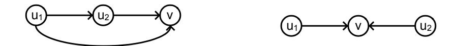
Figure 3: Parts of graph G such that sp,G(v) = 3
Case 1. Let there be a directed path of length 2 in G
Let us denote vertices as seen on the left in Figure 3. If we denote p(v) = a then p(u2) = a − 1 and p(u1) = a − 2. Since for G it holds n > 5 there have to be at least three other vertices u3, u4, u5 ∈ V (G). There can not be an arc which starts in u3 and ends in either u1, u2 or v
because it would increase the value sp,G(v). There also can not be an arc that starts in u2 or v and points to u3. In that case it would hold sp,G(u3) > sp,G(v). Thus, there must be an arc from u1 to u3 and p(u3) = a + 1. Let us consider vertex u4. For previous reasons, there can only be an arc between u3 and u4. If there is an arc u3u4, because of transitivity, there would also have to be an arc u1u4 and it would hold sp,G(u4) > sp,G(v). If there is an arc u4u3, then sp,G(u3) > sp,G(v) because p(u4) < a − 2. We have reached a contradiction.
Case 2. Let us assume that there is no directed path of lenght 2 in G and that there is a vertex of in-degree 2
Let us denote vertices as seen on the right in Figure 3. We can assume, without the lost of generality, that it holds p(u1) = a − 2 and p(u2) = a − 1. There must be vertex u3 ∈ V (G) but there can not be an arc which starts in u3 and ends in either u1, u2 or v because it would increase the value sp,G(v). There must also not be an arc from v to u3 because it would create a directed path of length 2. Let us consider two remaining possibilities: u1u3 ∈ E(G) or u2u3 ∈ E(G). Both situations are depicted on Figure 4.
- 1. Let us suppose there is an arc u1u3. There has to be a vertex u4 ∈ V (G). There can not be an arc u4v because it would increase the value sp,G(v). There also cannot be an arc u4u3 because p(u4) < a − 2. Thus, there must be an arc u2u4.
- 2. Let us suppose there is an arc u2u3. Analogous to previous considerations, there can only be an arc u2u4.
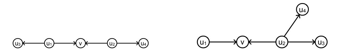
Figure 4: Examples of graphs G with n = 5 vertices such that s ∞(G) = 3
In both of these cases, there can not be any more vertices in V (G) in a way that s ∞(G) = sp,G(v) remains equal to 3.
Case 3. Let us assume that there is no directed path of lenght 2 and there is no vertex in V (G) with in-degree greater than 1
Let us denote by u and v vertices such that p(u) = p(v) − 3 and uv ∈ E(G). Let us denote p(v) = a. There must exist two vertices u1, u2 ∈ V (G) such that p(u1) = a − 1 and p(u2) = a − 2 and arcs uu1, uu2 ∈ E(G). Since n > 5 there also must exist a vertex u3 and an arc uu3. But p(u3) = a + 1 and thus sp,G(u3) > sp,G(v) which is again a contradiction.
The proofs for Theorems 3.10 and 3.11 follow directly from Theorem 3.9.
Theorem 3.10. Let G be a directed graph of type B with n > 5 vertices. It holds 2 ≤ a ∞(G). The lower bound is obtained for disoriented path.
Theorem 3.11. Let G be a directed graph of type B with n > 5 vertices. It holds 3 ≤ m∞(G). The lower bound is obtained for disoriented path.
Results for graphs of type B are summerized in Table 2.
| Measure | Minimal | Maximal |
|---|---|---|
| ∞(G) s | 4 | nP−1 i i=1 |
| ∞(G) a | 2 | n − 1 |
| m∞(G) | 3 | n − 1 |
| α s (G) | 2n−3 (*) n | !α!1 α Pn i −1 1 P j n i=2 j=1 |
| α a (G) | 1 (*) 2 | 1 nP−1 α 1 α i n i=1 |
| mα (G) | n−1 (*) n | 1 nP−1 α 1 α i n i=1 |
Table 2: Extremal values for the graphs of type B
Remark 3.1. Results marked (*) in Table 2 were stated and proven for α = 1, thus they remain an open problem for further investigation.
Discussions and conclusions
If we consider topological ordering as a process of arranging the vertices in the best possible way considering the constraints caused by the direction of edges, then it makes sense to try to optimize it by minimizing the distances between vertices in the ordering. This allows for a process that is represented by a directed acyclic graph to be more efficient (whether in execution time or in minimizing any cost function defined on the graph). For this purpose, we define measures for single vertices, generalize them to entire dags and bound their values over a set of all topological orderings of given dag. The results can be found in Tables 1 and 2. Results marked (*) in Table 2 were stated and proven for α = 1, thus they remain an open problem for further investigation. Potentially, the proved bounds could be used to benchmark existing algorithms, devise new approximation algorithms or branch–and–bound schemas for some scheduling problems which usually are of hard computational complexity.
Acknowledgement
This research is partially supported through project KK.01.1.1.02.0027, a project co-financed by the Croatian Government and the European Union through the European Regional Development Fund - the Competitiveness and Cohesion Operational Programme.
References
- [1] M. Albert and A. Frieze, Random graph orders, Order 6 (1989), 19–30.
- [2] S. Antunovic and D. Vuki ´ cevi ˇ c, Detecting communities in directed acyclic networks using ´ modified LPA algorithms, Proceedings of the 2nd Croatian Combinatorial Days (2019), 1– 14.
- [3] J. Bang–Jensen, Digraphs: Theory, Algorithms and Applications, Springer–Verlag (2008).
- [4] A. Barak and P. Erdos, On the number of strongly independent vertices in a directed acyclic ˝ random graph, SIAM J. Matrix Anal. A. 5 (1984), 508–514.
- [5] S. Baskiyar and R. Abdel-Kader, Energy aware DAG scheduling in heterogeneous systems, Cluster Computing 13 (2010), 373–383.
- [6] L. Bertacco, L. Brunetta, and M. Fischetti, The linear ordering problem with cumulative costs, Eur. J. Oper. Res., 189 (2008), 1345–1357.
- [7] B. Bollobas and G. Brightwell, The structure of random graph orders, SIAM J. Discrete Math. 10 (1997), 318–335.
- [8] P. Brucker, B. Jurisch, and B. Sievers, A branch and bound algorithm for the job–shop scheduling problem, Discrete Appl. Math. 49 (1994), 107–127.
- [9] M. Convolbo and J. Chou, Cost–aware DAG scheduling algorithms for minimizing execution cost on cloud resources, The Journal of Supercomputing 72 (2016), 985–1012.
- [10] H. El–Rewini, H.H. Ali, and T. Lewis, Task scheduling in multiprocessing systems, Computer 28 (1995), 27–37.
- [11] C. Hanen and A. Munier, A study of the cyclic scheduling problem on parallel processors, Discrete Appl. Math. 57 (1995), 167–192.
- [12] J. §. Ide and F. Cozman, Random generation of Bayesian networks, Proceedings of the 16th Brazilian Symposium on artificial intelligence (2002), 175–186.
- [13] F.V. Jensen, Bayesian Networks and Decision Graphs, Springer, Berlin, (2001)
- [14] B. Karrer and M. Newman, Random graph model for directed acyclic networks, Phys. Rev. E. 80 (2009)
- [15] H. Ke and B. Liu, Project scheduling problem with stochastic activity duration times, Appl. Math. Comput. 168 (2005), 342–353.
- [16] O. Mengshoel, D. Wilkins, and D. Roth, Controlled generation of hard and easy Bayesian networks: Impact on maximal clique size in tree clustering, Artificial Intelligence 170 (2006), 1137–1174
- [17] B. Pittel and R. Tungol, A phase transition phenomenon in a random directed acyclic graph, Random Struct. Algorithms 18 (2001), 164–184.
- [18] A. Quilliot and D. Rebaine, Linear time algorithms to solve the linear ordering problem for oriented tree based graphs, RAIRO–Oper. Res. 50 (2016), 315–325.
- [19] H. Topcouglu, S. Hariri, and M.–Y. Wu, Task scheduling algorithms for heterogeneous processors, Proceedings Eighth Heterogeneous Computing Workshop (1999), 3–14.
- [20] T. Łuczak, First order properties of random posets, Order 8 (1991), 291–297.