Christian Barrientos^a , Sarah Minion^b

^aValencia College, Orlando, FL 32832, U.S.A.

chr barrientos@yahoo.com, sarah.m.minion@gmail.com

Two of the most studied graph labelings are the types of harmonious and graceful. A harmonious labeling of a graph of size m and order n, is an injective assignment of nonnegative integers smaller than m, such that the weights of the edges, which are defined as the sum of the labels of the endvertices, are distinct consecutive integers after reducing modulo m. When n = m + 1, exactly two vertices of the graph have the same label. An α-labeling of a tree of size m is a bijective assignment of nonnegative integers, not larger than m, such that the labels on one stable set are smaller than the labels on the other stable set, and the weights of the edges, which are defined as the absolute difference of the labels of the end-vertices, are all distinct; this is the most restrictive type of graceful labeling. Even when these labelings are significantly different in their definitions of the weight, for certain kinds of graphs, there is a deep connection between harmonious and α-labelings. We present new families of harmoniously labeled graphs built on α-labeled trees. Among these new results there are three families of trees, the kth power of the path Pn, the join of a graph G and tK¹ where G is a graph that admits a more restrictive type of harmonious labeling and its order is different of its size by at most one unit. We also prove the existence of two families of disconnected harmonious graphs: Kn,m ∪K1,m−¹ and G∪T, where G is a unicyclic graph and T is a tree built with α-trees. In addition, we show that almost all trees admit a harmonious labeling.

Keywords: α-labeling, harmonious, strongly felicitous

Mathematics Subject Classification: 05C78

DOI: 10.5614/ejgta.2021.9.2.9

Received: 28 August 2020, Revised: 23 March 2021, Accepted: 13 April 2021.

^bFull Sail University, Winter Park, FL 32792, U.S.A.

1. Introduction

The process of labeling the vertices of a graph can be described as the assignment of labels to the vertices, usually nonnegative integers, that satisfies a number of conditions. In this work we study two of the most known of these assignments: graceful and harmonious labelings. Through the entire work we use the following conventions: a graph G has order n and size m if |V (G)| = n and |E(G)| = m. The stable sets of a bipartite graph G are the sets that form the natural bipartition of V (G); by Z^m we mean the set {0, 1, . . . , m − 1}.

The concept of graceful labeling was introduced in 1964 by Rosa [12]. Let G be a graph of size m. An injective function f : V (G) → Zm+1 is said to be graceful when every edge uv of G has assigned a weight defined as |f(u)−f(v)| and the set of all weights is {1, 2, . . . , m}. If such a labeling exists, then G is said to be a graceful graph. The complementary labeling of f, denoted by f and defined for each v ∈ V (G) by f(v) = m−f(v), is another graceful labeling of G. Note that if G is a tree, then f is a bijection. This shows that a forest with at least two components cannot be graceful. An open question in this subject is whether or not all trees are graceful.

A bipartite graceful graph G is called an α-graph if there exists a graceful labeling f of G with the additional property that there is an integer λ such that for every edge uv of G, f(u) ≤ λ < f(v) or f(v) ≤ λ < f(u). We refer to λ as the boundary value of f, and to the function as an α-labeling. Through this entire work, the symbol λ is reserved to represent the boundary value of the α-labeling under consideration. Let G be a tree of size m with stable sets A and B. Assuming that f is an α-labeling of G that assigns the label 0 to a vertex of A, there are some characteristics of f that is important to mention here:

• 1. The boundary value of f is λ = |A| − 1. (This implies that λ and |A| have different parity.)
• 2. The labels assigned by f to the vertices in A are 0, 1, . . . , λ; the labels assigned by f to the vertices in B are λ + 1, λ + 2, . . . , m.
• 3. The complementary labeling, f, assigns the label 0 to a vertex in B and its boundary value is m − λ. (This implies that for any α-tree, there exists an α-labeling that assigns the label 0 to a vertex in A.)

Rosa [12] showed that not all trees admit an α-labeling, he presented an infinite family of trees that are not α-graphs, the minimal member of this family is the tree obtained subdividing every edge of the star S³ ∼= K1,³ exactly once. An interesting fact is that any other subdivision of S³ results in an α-tree. Kotzig [11] proved that almost all trees admit an α-labeling. Although αlabelings are the most restrictive of the labelings introduced by Rosa, they are the most versatile in the sense that α-graphs are frequently used to construct new graceful or α-graphs. Furthermore, these labelings can be easily transformed into other types of labelings that, a priori, may seem unrelated. In [10], Lopez and Muntaner-Batle give a detailed account of the interaction of several ´ labelings, showing that α-labelings are the core of this research area and that the existence of a α-labeling of any graph implies the existence of many other types of labelings for that graph.

In 1980, Graham and Sloane [8] initiated the study of harmonious labelings of graphs. A graph G of size m is said to be harmonious if there is an injective function f : V (G) → Z^m such that when each edge uv ∈ E(G) is assigned the weight f(u) + f(v) reduced modulo m, the set of induced weights is Zm. With this definition, any graph of size m and order m + 1

cannot be harmonious; consequently, trees are not harmonious. In order to resolve this impasse, Graham and Sloane [8] modified the definition. They said that in the case of a tree, a harmonious labeling requires exactly one label to be repeated once. Naturally, this extension can be applied to any graph or order m + 1 and size m. In the same work, the authors conjectured that all trees are harmonious. This conjecture is still unproven but many families of harmonious trees have been discovered. Graham and Sloane proved that all caterpillars are harmonious. This result was extended by Figueroa-Centeno et al. [4]; these authors proved that any α-tree is also harmonious. Graham and Sloane [8] characterized harmonious cycles as those of odd size. So, an inevitable question is whether or not all unicyclic graphs are harmonious.

Another notational convention used in this paper is the following: If f is a labeling of G, either graceful or harmonious, the set of labels assigned by f to the vertices of G is denoted by L^f while W^f denotes the set of induced weights.

In this work, α-labeled trees are used to build new families of harmonious graphs. We prove in Section 2 that almost all trees are harmonious, as well as introduce three families of harmonious trees obtained from α-trees. Section 3 includes the construction of new families of harmonious unicyclic graphs and the study of the kth power of the path Pⁿ as a harmonious graph. In Section 4 we prove that the join G+nK¹ is harmonious when G is a strongly k-indexable graph such that its order and size differ by at most one unit. We close this work in Section 5 presenting two families of disconnected harmonious graphs: Kn,m ∪ K1,m−¹ and G ∪ T, where G is a unicyclic graph and T is a tree satisfying certain conditions. This last result is a corollary of one of the conclusions in Section 2.

All graphs considered in this work are finite, with no loops nor multiple edges. All graph theoretical notation not given here is taken from [2] and [5]. The reader interested in this subject may find more information in Gallian' survey [5], which is updated annually.

2. Harmonious Trees

Are all trees graceful? Are all trees harmonious? Both questions have been the center of several papers in the last decades; a good amount of results are known with respect to graceful labelings and in particular about α-trees. It is well-known that in the case of trees, the existence of an α-labeling implies the existence of an harmonious labeling, therefore many families of trees are known to admit this kind of labeling. In this section, we use this property to show that almost all trees are harmonious and also, to present three new techniques that will allow us to produce families of harmonious trees.

2.1. Almost all Trees are Harmonious

Slightly different of harmonious labelings are those called felicitous. Let G be a graph of order n and size m, an injective function f : V (G) → Zm+1 is called felecitous if the weights induced by f(u) + f(v) (mod m) on each edge uv ∈ E(G) are all distinct, i.e., they form the set Zm. In [4], Figueroa-Centeno et al., studied a more restrictive felicitous labeling; they said that a felicitous labeling is strongly felicitous if there exists an integer κ such that for every edge uv, min{f(u), f(v)} ≤ κ < max{f(u), f(v)}. Note the strong similarity between the parameters λ

and κ. They prove the following result that connects this type of labeling with the well-known α-labeling.

Theorem 2.1. A graph of order n and size m, with m ≥ n − 1, is strongly felicitous if and only if it is an α-graph.

Trees satisfy this constraint on the order and the size, therefore we have the following corollary.

Corollary 2.1. If T is an α-tree, then T is strongly felicitous.

For the sake of completeness we show a way to transform an α-labeling into a strongly felicitous labeling. Suppose that f is an α-labeling of a tree of size m and v ∈ V (T). Then a strongly felicitous labeling g of T is given by:

\[g(v_i) = \begin{cases} f(v), & \text{if } f(v) \le \lambda, \\ m + \lambda + 1 - f(v), & \text{if } f(v) > \lambda. \end{cases}\]

In [11], Kotzig proved that almost all trees admit an α-labeling. Since every α-labeling of a tree can be transformed into a strongly felicitous labeling, we conclude that almost all trees are strongly felicitous. We use this fact to prove that almost all trees are harmonious.

Theorem 2.2. Almost all trees are harmonious.

Proof. Let f be an α-labeling of a tree T of size m. Since f can be transformed into the strongly felicitous labeling g described before, we know that L^g = Zm+1 and W^g = Zm. Thus, by reducing the elements of L^g modulo m, we get that only the label 0 is used twice. So, in this modified labeling the set of labels is Zm. Let v ∈ V (G) such that g(v) = m and e = uv any edge incident to v. Then, the weight of e under the original labeling g is g(u) + g(v) = g(u) + m ≡ g(u)(mod m). By making g(v) = 0, the previous congruence remains unchanged, implying that the weight of e is still the same. Therefore, the set of weights is Z^m and the modified function g is a harmonious labeling of G. Consequently, each α-labeling of G can be transformed into a harmonious labeling, proving in this way that almost all trees are harmonious.

In the following theorem, we introduce a simple procedure that allows us to build harmonious trees from an existing α-labeled tree. We include this theorem in this subsection just to emphasize the fact that α-labelings can be used to generate larger harmonious graphs in contrast with the previous result where we modified the labeling but not the graph.

Theorem 2.3. Let T be a tree and e an edge of T incident to a leaf. If T − e is an α-tree, then T is harmonious.

Proof. Suppose that T is a tree of size m + 1 such that there exists an edge e = uv in T, where deg(u) = 1 and T ⁰ = T − e is an α-tree. Let f be an α-labeling of T 0 , when f is transformed into the strongly felicitous labeling g, the vertices of T 0 are labeled injectively with the elements of Zm+1; in addition,

\[\{g(u) + g(v) : uv \in E(T')\} = \{\lambda + 1, \lambda + 2, \dots, \lambda + m\},\\]

when these weights are reduced modulo m+1, we get the set \(\mathbb{Z}_{m+1}-\{\lambda\}\).

We extend the labeling g to the vertices of T in the natural way. That is, every vertex of T' keeps its label in T. Recall that \(u \notin V(T')\). Assume that g(v) = a; since the equation \(x + a = \lambda\) always has a solution in \(\mathbb{Z}_{m+1}\), the integer x can be used to label the other end-vertex of e, that is, we make g(u) = x. In this way, the edge e has weight \(\lambda\) and the only label used twice is x. Thus, the labeling g is harmonious. Therefore, T is a harmonious tree.

In Figure 1 we show an example of this construction. The figure on the top left corner is the \(\alpha\)-labeled tree T', the other seven figures are trees of size 12 that satisfy the hypothesis of the theorem; i.e., if the red edge is deleted, the underlying tree is the same \(\alpha\)-tree T'.

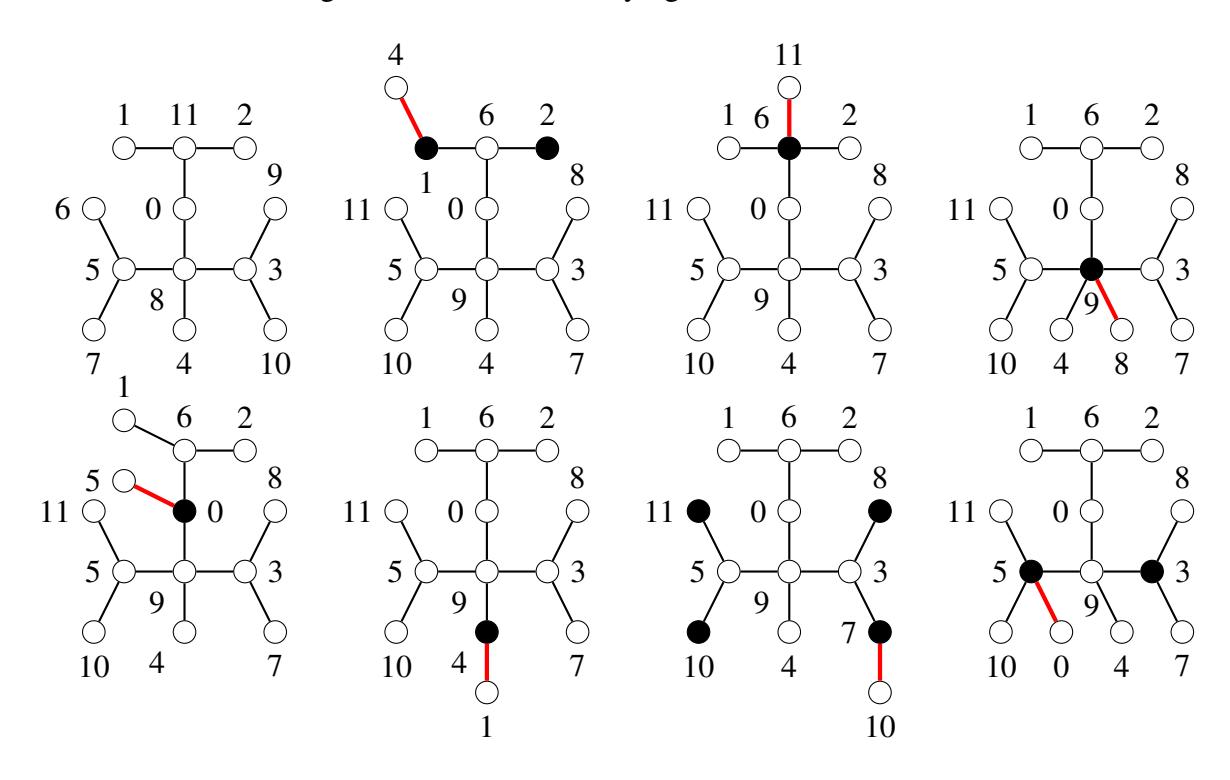
Figure 1. All the harmoniously labeled trees of size 12 obtained from the same \(\alpha\)-labeled tree of size 11.

2.2. New Families of Harmonious Trees

In this subsection we continue the idea of attaching pendent vertices to the vertices of an \(\alpha\)-tree to produce new harmonious trees. In our next theorem, we are attaching \(x \geq 1\) pendent vertices to an \(\alpha\)-tree generating in this way a tree of size m + x.

Suppose that T is an \(\alpha\)-tree of size m with stable sets A and B, where a=|A| and b=|B|. If f is an \(\alpha\)-labeling of T, then its boundary value equals a-1 or b-1, depending on which of the stable sets has the vertex labeled \(\lambda\). Let \(\mathscr{T}_i\) denote the family of trees obtained from T by attaching a pendent vertex to each of k vertices of A and to each of k-i vertices of B, where \(1 \le k \le \min\{a,b\}\) and \(i \in \{0,1\}\). The tree \(T_i\) has size m+2k-i. We claim that for each \(\alpha\)-tree T and every \(i \in \{0,1\}\) there exists a harmonious tree \(T_i \in \mathscr{T}_i\).

Proof. Suppose that T is a tree of size m with stable sets A and B, and f is an α-labeling of T that assigns the label 0 to a vertex in A. Select a positive number k such that k ≤ min{|A|, |B|}. First, we construct a harmoniously labeled tree T0. Once this is done, we transform T⁰ into a tree T1.

We start converting f into the strongly felicitous labeling g described above. Therefore, L^g = Zm+1; moreover, the labels assigned by g to the vertices in A are 0, 1, . . . , |A| − 1, and to the vertices in B are |A|, |A| + 1, . . . , m. We identify each vertex of T with its corresponding label, that is, for each i ∈ Zm+1, the vertex i is the vertex labeled i by the function g.

A tree T⁰ is built by adding a pendent vertex to each of 2k vertices of T, k on each stable set. Since our goal is to get a harmonious tree, the selected vertices of T are: λ − k + 1, λ − k + 2, . . . , λ+k. Note that the vertices λ−k+1, λ−k+2, . . . , λ are in A while the remaining vertices are in B. Attach a pendent vertex to each of the selected vertices. The corresponding labels of the pendent vertices attached to the elements of A are: m + k, m + k + 1, . . . , m + 2k − 1. Thus, the weights of the new edges are: m + λ + 1, m + λ + 3, . . . , m + λ + 2k − 1, respectively. The labels of the pendent vertices attached to the elements of B are: m + 1, m + 2, . . . , m + k. Consequently, the induced weights of these new edges are: m + λ + 2, m + λ + 4, . . . , m + λ + 2k.

Hence, the new labels are in the range {m + 1, m + 2, . . . , m + 2k − 1}. Since the new tree has size m + 2k, the maximum label assigned to a vertex of T⁰ is smaller than its size. In addition, the weights of the new edges are m + λ + 1, m + λ + 2, . . . , m + λ + 2k and on the edges of T are λ + 1, λ + 2, . . . , m + λ. Therefore, the tree T⁰ is harmoniously labeled because the only label repeated twice is m + k, this label has been assigned to the pendent vertices attached to λ − k + 1 and λ + k.

Now, delete from T⁰ the vertex labeled m + k attached to the vertex λ + k of B. The new tree is of the type T¹ ∈ T1, which implies that its size is m + 2k − 1, but this number coincides with the largest label used. Recall that this label was used on the pendent vertex attached to λ. So, if we reduce this number modulo m + 2k − 1, it becomes the number 0 and the pendent edge has now weight λ. This means that the labeling of T¹ assigns labels from {0, 1, . . . , m + 2k − 2}, being 0 the only label used on two vertices, and the induced weights are now λ, λ + 1, . . . , m + 2k − 2. Therefore, T¹ is a harmonious tree.

In Figure 2 we show an example of the harmoniously labeled trees T⁰ and T¹ obtained from an α-tree of size 11, with |A| = 5, |B| = 7, λ = 4 and k = 4. We start exhibiting the α-labeling of T, the edges added to T to build T⁰ and T¹ are in blue and red; the vertices with repeated labels are in black.

In the following theorem we explore a method to build harmonious trees that can be described as the one-point union of an odd number of copies of an α-tree of even size. The resulting labeled tree has some properties that allow us to transform it into a disconnected graph, that is the union of a unicyclic graph and a tree, and also into a unicyclic graph. In both cases, the final graph is harmonious.

Theorem 2.5. Suppose that f is an α-labeling of a tree G of even size m. If k > 1 is odd, then a harmonious tree of size k(m + 1) can be built with k copies of G by connecting a new vertex to the vertex labeled λ in ^k+1 2 of the copies of G and the vertex labeled m in the remaining ^k−¹ 2 copies.

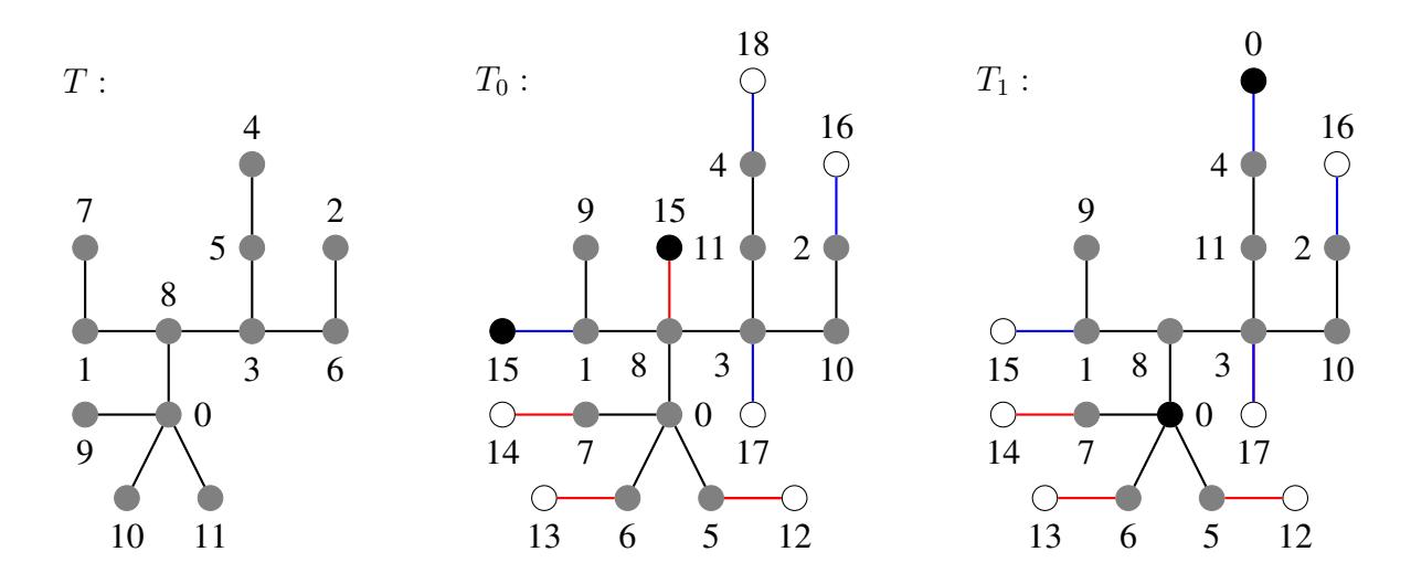
Figure 2. An \(\alpha\)-tree T and two harmoniously labeled trees \(T_0\) and \(T_1\).

Proof. Let G be an \(\alpha\)-tree of even size m; then the stable sets of G have cardinalities with different parities. Suppose that f is an \(\alpha\)-labeling of G such that \(\lambda\) is assigned to a vertex of the stable set with an odd number of elements; this implies that \(\lambda\) is even. If g is the strongly felicitous labeling of G obtained from f, then \(L_g = \{0, 1, \ldots, m\}\) and \(W_g = \{\lambda + 1, \lambda + 2, \ldots, \lambda + m\}\).

For each \(i \in \{1, 2, \dots, k\}\), let \(G_i\) be a copy of G and \(h_i\) be the labeling defined for every \(v \in V(G_i)\) as \(h_i(v) = kg(v) + i - 1\). Thus, \(L_{h_i} = \{i - 1, k + i - 1, \dots, km + i - 1\}\) and the union of the sets \(L_{h_i}\) is \(\{0, 1, \dots, k(m+1) - 1\}\). Consequently, the labeling of \(\bigcup_{i=1}^k G_i\) is an increasing function, implying that \(G_1\) has the edge with the smallest weight and \(G_k\) has the edge with the largest weight; these weights are \(k(\lambda + 1)\) and \(k(\lambda + m) + 2(k - 1)\), respectively.

Suppose that \(e = uv \in E(G)\) has weight w, with w = g(u) + g(v). Then, when e is seen as an edge of \(G_i\), its weight is

\[h_i(u) + h_i(v) = (kg(u) + i - 1) + (kg(v) + i - 1)\]
= \(k(g(u) + g(v)) + 2(i - 1)\)
= \(kw + 2(i - 1)\).

This implies that if \(e_1, e_2 \in E(G)\) have weights w and w+2 under the labeling g, then the set formed by the weights of the replicas of \(e_1\) in all the graphs \(G_i\) is \(E_1 = \{kw, kw+2, \ldots, kw+2(k-1)\}\); similarly we get that \(E_2 = \{k(w+2), k(w+2)+2, \ldots, k(w+2)+2(k-1)\}\). Note that \(E_1 \cap E_2 = \varnothing\) and \(E_1 \cup E_2\) is a set of consecutive integers with the same parity.

Since \(\lambda\) is even, \(\lambda+1\) and \(\lambda+m-1\) are the smallest and largest odd weights induced by g on the edges of G, while \(\lambda+2\) and \(\lambda+m\) are the smallest and largest even weights. Thus, the weights of the edges of \(\bigcup_{i=1}^k G_i\) can be separated into three disjoint sets:

\[S_{1} = \{k(\lambda + 1), k(\lambda + 1) + 2, \dots, k(\lambda + 2) - 1\},\] \[S_{2} = \{k(\lambda + 2), k(\lambda + 2) + 1, \dots, k(\lambda + m - 1) + 2(k - 1)\},\] \[S_{3} = \{k(\lambda + m - 1) + 2(k - 1) + 1, k(\lambda + m - 1) + 2(k - 1) + 2, \dots, k(\lambda + m) + 2(k - 1)\}.\]

Note that \(|S_1| = |S_3| = \frac{k+1}{2}\), \(|S_2| = k(m-1)-1\), and \(S = S_1 \cup S_2 \cup S_3\) is not a set of consecutive integers but its complement with respect to \(\{k(\lambda+1), k(\lambda+1)+1, \dots, k(\lambda+m)+2k-1\}\) is \(M = \{k(\lambda+1)+1, k(\lambda+1)+3, \dots, k(\lambda+2)-2\} \cup \{k(\lambda+m-1)+2(k-1)+2, k(\lambda+m-1)+2(k-1)+2, k(\lambda+m-1)+2(k-1)+3, \dots, k(\lambda+m)+2(k-1)+1\}\).

Now that the vertices of \(\bigcup_{i=1}^k G_i\) have been labeled, we introduce a new vertex, labeled 0. If u is the vertex of G with label \(g(u) = \lambda + 1\), we connect the new vertex with each replica of u on \(G_2, G_4, \ldots, G_{k-1}\), which labels are \(k(\lambda+1)+1, k(\lambda+1)+3, \ldots, k(\lambda+2)-2\), producing edges with weights identical to these labels. If v is the vertex of G with label \(g(v) = \lambda\), we connect the new vertex with each copy of v on \(G_1, G_3, \ldots, G_k\) generating edges with weights \(k\lambda, k\lambda+2, \ldots, k(\lambda+1)-1\). By adding the constant k(m+1) to these numbers we get

\[k\lambda + k(m+1) = k(\lambda + m - 1) + 2(k - 1) + 2\]\[k\lambda + 2 + k(m+1) = k(\lambda + m - 1) + 2(k - 1) + 4\]\[\vdots\]\[k\lambda + k - 1 + k(m+1) = k(\lambda + m) + 2(k - 1) + 1.\]

In other terms, the weights of the new edges are precisely the elements of M. Hence the graph obtained is a tree of size k(m+1), labeled with the elements of \(\mathbb{Z}_{k(m+1)}\), where 0 is the only label used twice, and the set formed by all the induced weights is \(\{k(\lambda+1), k(\lambda+1)+1, \ldots, k(\lambda+m)+2k-1\}\). When the elements of this set are reduced modulo k(m+1) we get the elements of \(\mathbb{Z}_{k(m+1)}\), which implies that the new tree is harmonious.

In Figure 3 we show an example of this construction for a graph built with k = 11 copies of \(G \cong P_3\). The edges in red correspond the the copy \(G_1\) of \(P_3\). This copy plays an important role in the following corollaries.

Suppose that the copy \(G_1\) of G is not connected to the new vertex 0. Recall that the labels of \(G_1\) are \(0, k, \ldots, km\) and that by disconnecting \(G_1\) from the tree we lost the edge of weight \(k\lambda\). So, by connecting the vertices of \(G_1\) labeled 0 and \(k\lambda\) we get a unicyclic graph with weights \(k\lambda, k(\lambda+1), \ldots, k(\lambda+m)\). Note that the union of this graph and the tree formed by \(G_2, G_3, \ldots, G_k\), is a harmonious disconnected graph.

Once the unicyclic graph formed with \(G_1\) is in place, we can identify (amalgamate) its vertex labeled 0 with the vertex labeled 0 in the subtree created with \(G_2, G_3, \ldots, G_k\), to generate a harmonious unicyclic graph. Thus, we have the following corollaries.

Corollary 2.2. Let T be the harmoniously labeled tree attained in Theorem 2.5. If the two vertices of T labeled 0 are identified, then a harmonious unicyclic graph is obtained.

Corollary 2.3. Let G be the harmoniously labeled unicyclic graph attained in Corollary 2.2. If G is decomposed into a cycle and a tree, then the disconnected graph obtained is also a harmonious unicyclic graph.

3. \(\alpha\)-Trees and Harmonious Graphs

In this section we explore two techniques used to construct harmonious graphs by modifying the \(\alpha\)-labeling of a tree. We open the section by building some families of harmonious unicyclic

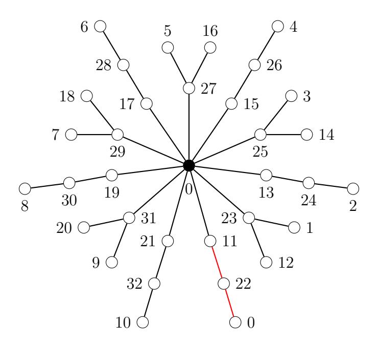
Figure 3. Harmonious labeling of a tree built with 11 copies of P3.

graphs. At the end of the section we prove that the kth power of the path Pⁿ is a harmonious graph for feasible values of n and k.

Graham and Sloane [8] proved that all caterpillars are harmonious and conjectured that all trees are harmonious. As we showed in Section 2, almost all trees are harmonious because almost all trees admit α-labelings. A natural question related to trees and cycles is whether or not all unicyclic graphs are harmonious as well. The answer is not, because the even cycles (i.e., cycles of even size) were proved to be not harmonious in [8]. Are the even cycles the only exception within the family of unicyclic graphs?

We open this section presenting two constructions of unicyclic harmonious graphs based on the α-labelings of caterpillars discovered by Rosa [12]. Given the simplicity of these constructions, we omit the proof of any result associated with them; instead we provide an example to explain how these constructions work. Consider the strongly felicitous labeled graph G of size 23 and diameter 9 shown in Figure 4. This graph G has a symmetry with respect to its center (red edge), that is, if e is the center of G, then the two components of G − e are isomorphic. The set of weights is {12, 13, . . . , 34}. The black vertices have labels 0, 1, . . . , 11; so, among these numbers there are six pairs x, y such that x + y = 11. Since the vertices labeled x and y are in the same stable set of G, they are not adjacent. Therefore, by adding an edge connecting them we obtain a harmonious unicyclic graph. Note that we have not yet used the symmetry, which means that the construction just described can be applied to any caterpillar. In the second part of Figure 4 we show the six unicyclic graphs described before, to avoid duplication of weights we must take one dashed blue edge at a time.

The second construction uses the symmetry of G. We must observe that every vertex v of the

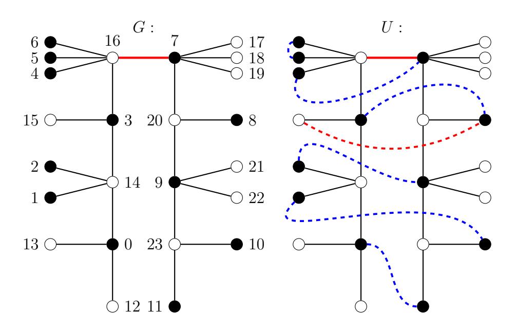
Figure 4. Strongly felicitous labeled caterpillar and some unicyclic graphs built on it.

left side of the red edge has a replica v' on the right side; if we connect v and v', an edge with the same weight that the red edge is introduced, which means that the red edge can be replaced by any of these edges without affecting the harmoniousness of the unicyclic graph. We show this fact in the second part of Figure 4, where a red dashed edge has been introduced. In general, many of the unicyclic graphs so obtained are non-isomorphic, everything depends on the structure of the graph. In the specific case of our graph G, there are 66 non-isomorphic unicyclic harmoniously labeled graphs that have the labeling of G as their base.

Theorem 3.1. If T is an \(\alpha\)-tree with stable sets of cardinalities r and s, then there exist \(\lfloor \frac{r}{2} \rfloor + \lfloor \frac{s}{2} \rfloor\) harmoniously labeled unicyclic graphs that have T as a spanning tree.

Proof. Suppose that T is an \(\alpha\)-tree with stable sets R and S such that |R| = r and |S| = s. Then, there exists an \(\alpha\)-labeling f of T that assigns the integers in \(L_R = \{0, 1, \ldots, r-1\}\) to the elements of R and the integers in \(L_S = \{r, r+1, \ldots, r+s-1\}\) to the elements of S. Let g be the strongly felicitous labeling of T obtained from f as described above. Thus, the labels on each stable set are the same as before and the set of induced weights is \(\{r, r+1, \ldots, 2r+s-2\}\).

In \(L_R\) there are \(\lfloor \frac{r}{2} \rfloor\) pairs x,y such that x+y=r-1. Let \(u_R,v_R\) be elements of R such that \(g(u_R)+g(v_R)=r-1\), since these vertices are not adjacent, the introduction of the new edge \(u_Rv_R\) results in a unicyclic graph of odd girth. The weights on the edges of this graph form the set \(\{r-1,r,\ldots,2r+s-2\}\), therefore the graph is harmonious. In \(L_S\) there are \(\lfloor \frac{s}{2} \rfloor\) pairs x,y such that x+y=2r+s-1; as we did before, take any two vertices in S, say \(u_S,v_S\) satisfying \(g(u_S)+g(v_S)=2r+s-1\) and connect them to produce a harmoniously labeled unicyclic graph where the set of induced weights is \(\{r,r+1,\ldots,2r+s-1\}\).

Summarizing, the new edge can be drawn in \(\lfloor \frac{r}{2} \rfloor + \lfloor \frac{s}{2} \rfloor\) ways, and each of these alternatives

generates a unicyclic graph where T is one of its spanning trees. Note that as graphs, they may be isomorphic, but as labeled graphs they are different.

In Figure 5 we show an example of this last result for a tree T where r = s = 5. In the first part we show the α-labeling of T. In the second part we show the strongly felicitous labeling of T together with four possible new edges, such that the selection of any of them results in a harmoniously labeled unicyclic graph.

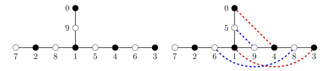
Figure 5. An α-labeled tree and four harmoniously labeled unicyclic graphs.

Another harmonious unicyclic graph can be obtained by starting with an α-labeled tree and identifying the vertices labeled 0 and λ + 1 when they are at distance at least 3.

Theorem 3.2. Let T be a tree and f be an α-labeling of T. If the vertices labeled 0 and λ + 1 by f are at distance at least three, then the unicyclic graph formed by identifying these vertices is harmonious.

Proof. Suppose that T is a tree of size m and f be an α-labeling of T. Let u, v denote the vertices of T such that f(u) = 0 and f(v) = λ + 1. Suppose that dist(u, v) ≥ 3. When f is transformed into the strongly felicitous labeling g given in Section 2, we get g(u) = 0 and g(v) = m. By making the label m equal to 0, we transform g into a harmonious labeling of T. When the two vertices of T labeled 0 are identified, a unicyclic graph with girth dist(u, v) is created. Since no new edge has been added, the labeling of this graph keeps its harmonious characteristic.

The kth power of the path Pn, denoted by P k n , is the graph obtained from Pⁿ by adding the edges that connect all vertices at distance k. Grace [7] proved that P 2 n is harmonious. The set formed by all the graphs P 2 n is a subfamily of the polyiamonds, i.e., those connected planar graphs formed with copies of the cycle C³ (or triangle) amalgamating edges. A graph of this family is said to be a n-cell snake polyiamond if it is built with n triangles and every triangle shares at most two edges with its neighbors. Thus, P 2 n is one special case of snake polyiamond, where the largest degree is 4. Recently, Barrientos [1] extended Grace's result by proving that all snake polyiamonds are harmonious. Seoud et al. [14] proved that P 3 n is harmonious. Gallian [5] mentioned that in [18], Youssef generalized this result by proving that P k n is harmonious when k is odd. We have not found this result in Youssef's paper. In the following theorem we prove that P k n is harmonious when k is even. So, if the case k odd was in fact proved, we could say that the kth power of the path Pⁿ is harmonious for every n ≥ 3.

Theorem 3.3. The kth power of the path of order n, \(P_n^k\) is a harmonious graph for every \(n \ge 3\) and \(k \le n - 1\) even.

Proof. Since the case k=2 was proven in [7] and \(P_n^k \cong C_n\) when k=n-1 and these cycles are harmonious , we are going to assume that \(n\geq 5\) and \(4\leq k< n-1\).

Let \(v_1, v_2, \ldots, v_n\) be the consecutive vertices of the path \(P_n\), in order to form the graph \(G = P_n^k\) we add the edges \(v_i v_{i+k}\) for every \(i \in \{1, 2, \ldots, n-k\}\). Thus, G is a graph of order n and size 2n-1-k. Consider the following labeling of the vertices of \(P_n\):

\[f(v_i) = \begin{cases} \frac{i-1}{2}, & \text{if } i \text{ is odd,} \\ \frac{2n+i-k-2}{2}, & \text{if } i \text{ is even and } n \text{ is odd,} \\ \frac{2n+i-k-4}{2}, & \text{if } i \text{ is even and } n \text{ is even.} \end{cases}\]

Note that each part of this function is linear and increasing. Due to the fact that the values assigned by f on the vertices of G are affected by the parity of n, we analyze each possibility independently.

Suppose that n is odd. Since the definition of f depends on the parity of i we have that \(\{0,1,\ldots,\frac{n-1}{2}\}\) is the set formed by the labels assigned by f on the vertices with an odd index, while \(\{\frac{2n-k}{2},\frac{2n+2-k}{2},\ldots,\frac{3n-3-k}{2}\}\) is formed by the labels on the vertices with an even index. By hypothesis, we know that

\[k \le n-1 \Leftrightarrow 1 \le n-k \Rightarrow -1 < n-k \Leftrightarrow n-1 \le 2n-k \Leftrightarrow \frac{n-1}{2} \le \frac{2n-k}{2}.\]

This proves that these two sets are disjoint, which means that the function is injective. In addition, we can see that the maximum label on a vertex of G is \(\frac{3n-3-k}{2}\), which is smaller than 2n-1-k because \(k \leq n-1\). Consequently, f is an injective function whose range is a subset of \(\{0,1,\ldots,2n-2-k\}\).

Now we study the weights induced by f. Seeing that for each parity of i, the vertices \(v_i\) and \(v_{i+2}\) are labeled with consecutive integers, the weights on the edges \(v_i v_{i+1}\) (i.e., the edges of \(P_n\)) are the integers \(\frac{2n-k}{2}, \frac{2n-k}{2}, +1, \ldots, \frac{4n-4-k}{2}\); when these numbers are reduced modulo 2n-1-k we get the set \(\{\frac{2n-k}{2}, \frac{2n-k}{2}+1, \ldots, 2n-2-k\} \cup \{0,1,\ldots,\frac{k}{2}-1\}\). Since k is even, and regardless the parity of i, the edges \(v_i v_{i+k}\) and \(v_{i+2} v_{i+2+k}\) have weights that are consecutive integers with the same parity as \(\frac{k}{2}\). In particular, when i is odd, the weights on the edges \(v_i v_{i+k}\) form the set \(\{\frac{k}{2}, \frac{k}{2}+2, \ldots, \frac{2n-k}{2}-1\}\); when i is even the weights are \(\frac{4n-k}{2}, \frac{4n-k}{2}+2, \ldots, \frac{6n-6-3k}{2}\). Reducing these numbers modulo 2n-1-k we obtain the elements of the set \(\{\frac{k}{2}+1, \frac{k}{2}+3, \ldots, \frac{2n-k}{2}-2\}\). The union of all these sets is \(\{0,1,\ldots,2n-2-k\}\); consequently, f is a harmonious labeling of G when n is odd.

Suppose now that n is even. We follow the same steps that in the previous case. The vertices \(v_i\) receive the labels from \(\{0,1,\ldots,\frac{n}{2}-1\}\) when i is odd and from \(\{\frac{2n-k}{2}-1,\frac{2n-k}{2},\ldots,\frac{3n-4-k}{2}\}\) when i is even. As before, these are disjoint sets and the function is injective, the largest label is \(\frac{3n-4-k}{2}\) which is smaller than 2n-1-k. The weights on the edges \(v_iv_{i+1}\) are \(\frac{2n-k}{2}-1,\frac{2n-k}{2},\ldots,\frac{4n-6k}{2}\);

when these numbers are reduced modulo 2n-1-k we get the set \(\left\{\frac{2n-k}{2}-1,\frac{2n-k}{2},\dots,2n-2-k\right\}\cup\{0,1,\dots,\frac{k}{2}-2\}\). For i odd, the weights on the edges \(v_iv_{i+k}\) form the set \(\left\{\frac{k}{2},\frac{k}{2}+2,\dots,\frac{2n-k}{2}-2\right\}\). When i is even, the weights on these edges are \(\frac{4n-k}{2}-2,\frac{4n-k}{2},\dots,\frac{6n-8-3k}{2}\); again, reducing modulo 2n-1-k we get the set \(\left\{\frac{k}{2}-1,\frac{k}{2}+1,\dots,\frac{2n-k}{2}-3\right\}\). Then, the union of these sets is \(\{0,1,\dots,2n-2-k\}\) and f is a harmonious labeling when n is even.

In Figure 6 we show an example of this labeling for the graph \(P_{19}^{10}\).

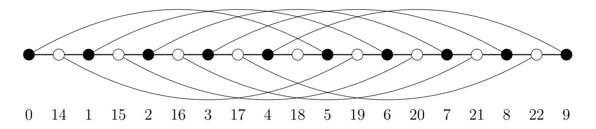
Figure 6. Harmonious labeling of \(P_{19}^{10}\).

4. The Join Product with Harmonious Graphs

Recall that the join of simple graphs G and H, written G+H, is the graph obtained from the disjoint union \(G \cup H\) by adding the edges \(\{uv : u \in V(G), v \in V(H)\}\). When T is a tree of size m, the join \(T+K_1\) is a graph of order m+2 and size 2m+1. This implies that the maximum label allowed in a harmonious labeling of this graph is 2m.

We can find in the literature several results about the join of two graphs. For instance, we know that the following graphs are harmonious: \(nC_m + K_1\) for every \(n \not\equiv 0 \pmod{4}\) [3], \(K_{m,n} + K_1\) [16], \(K_{m,n} + K_2\) [17], \(K_2 + K_2 + \cdots + K_2\) [9], \(P_n + K_2\) [13], \(P_n + K_1\) and \(C_n + K_1\) [8], \(C_m + nK_1\) if m is odd [15], \(S_m + nK_1\) and \(P_m + nK_1\) [6]. The trees used in the last two graph families correspond to instances of \(\alpha\)-trees; in the following results we prove that \(T + nK_1\) is harmonious when T is any \(\alpha\)-tree of size m, superseding the ones given in [6].

Lemma 4.1. If T is an \(\alpha\)-tree, then the join \(T + K_1\) is harmonious.

Proof. Suppose that T is an \(\alpha\)-tree of size m and f is an \(\alpha\)-labeling of T with boundary value \(\lambda\). We convert f into the strongly felicitous labeling g. In this way, the labels assigned by g are \(0, 1, \ldots, m\) and the induced weights are \(\lambda + 1, \lambda + 2, \ldots, \lambda + m\).

Now, the labels assigned by g are shifted \(m-\lambda\) units. So, the new labels are \(m-\lambda, m-\lambda+1,\ldots,2m-\lambda\), and the new weights are \(2m-\lambda+1,2m-\lambda+2,\ldots,2m-\lambda+m=3m-\lambda\). Since \(\lambda\geq 0\), the maximum label assigned, i.e., \(2m-\lambda\), is smaller than the size of the graph.

The vertex of \(K_1\) is labeled 0. In this way, the edges connecting this vertex with the vertices of T have weights \(m - \lambda, m - \lambda + 1, \dots, 2m - \lambda\). Which implies that the weights induced on the edges of \(T + K_1\) are \(m - \lambda, m - \lambda + 1, \dots, 3m - \lambda\), that is, 2m + 1 consecutive integers. When

these numbers are reduced modulo 2m + 1 they form the set {0, 1, . . . , 2m}. Since all the labels are distinct and are in the range {0, 1, . . . , 2m − λ} where 2m − λ ≤ 2m because λ ≥ 0, we get that T + K¹ has been harmoniously labeled.

As an example, the labeling of T + K¹ is shown in Figure 7, where T, depicted with black edges, is an α-tree of size m = 12; its original α-labeling has boundary value λ = 4.

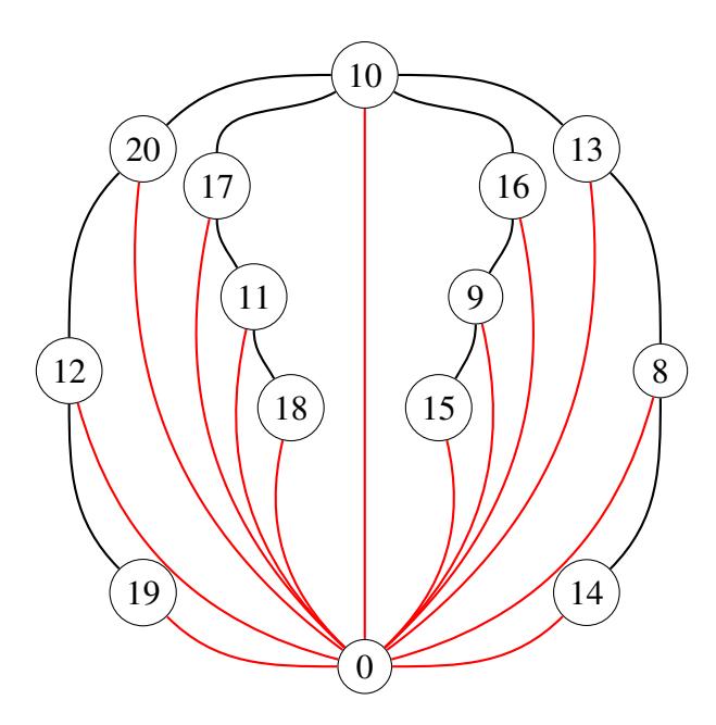
Figure 7. Harmonious labeling of a graph T + K1.

Now that a harmonious labeling of T + K¹ is known, it is easier to build a harmonious labeling of the general case T + nK¹ for every n ≥ 2. Note that this join has order m + n + 1 and size m + n(m + 1).

Theorem 4.1. If T is an α-tree, then the join T + nK¹ is harmonious for every n ≥ 2.

Proof. Let T be a tree of size m that admits an α-labeling with boundary value λ. Suppose that a harmonious labeling of T + K¹ has been obtained using the procedure explained in the proof of Lemma 4.1. Thus, the labels on the vertices of T form the set {m − λ, m − λ + 1, . . . , 2m − λ} and the largest weight on an edge of T is 3m − λ. If v2, v3, . . . , vⁿ are the, still unlabeled vertices of nK1, we assign to each vⁱ the label (m + 1)i − 1. Note that all these labels are different, being 2m + 1 the smallest, which is larger than 2m −λ, and the largest is (m + 1)n−1, which is smaller than the size of T + nK1.

Furthermore, the edges connecting vⁱ to T have weights that are consecutive integers and form the set

\[W_i = \{(m+1)i - 1 + m - \lambda, \dots, (m+1) - 1 + 2m - \lambda\}\]
= \{m(i+1) + i - 1 - \lambda, \dots, m(i+2) + i - 1 - \lambda\}.

Since for every i ∈ {2, 3, . . . , n − 1}, max(Wi) = m(i + 2) + i − 1 − λ and min(Wi+1) = m(i + 2) + i − λ, differ by exactly one unit, we get

\[\bigcup_{i=2}^{n} W_i = \{3m - \lambda + 1, \dots, (n+2)m + n - 1 - \lambda\},\\]

i.e., a set of (m+1)(n−1) consecutive integers, which are consecutive with the weights on T +K1. Therefore, the labeling of T + nK¹ is harmonious.

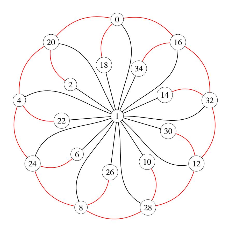
Figure 8. Harmonious labeling of (C⁹  K1) + K1.

A similar result can be obtained if the tree T is replaced by a unicyclic harmonious graph. We prove this claim in the upcoming theorem.

Theorem 4.2. If G is a harmonious unicyclic graph, then G + nK¹ is harmonious.

Proof. Suppose that G is a harmonious graph of size m. If f is a harmonious labeling of G, then the labels assigned by f are 0, 1, . . . , m−1 and the induced weights are also 0, 1, . . . , m−1. Let g be the labeling of G defined for every v ∈ V (G) as g(v) = (n + 1)f(v). The new labels are 0, n + 1, . . . ,(m − 1)(n + 1) and the induced weights form the set W = {0, n + 1, . . . ,(m − 1)(n + 1)}.

The join G + nK¹ has size m(n + 1); so, the largest label assigned by g is n units smaller than the size.

The vertices of nK¹ are labeled by g with the integers 1, 2, . . . , n. Thus, the labels are in the range allowed by a harmonious labeling. Note that for each i ∈ {0, 1, . . . , m − 1}, the edges connecting the vertex of G labeled i(n + 1) with the vertices of nK¹ have weights that form the set Wⁱ = {i(n + 1) + 1, i(n + 1) + 2, . . . , i(n + 1) + n}. Hence, the union of these sets with W produces a set with elements 0, 1, 2, . . . ,(m −1)(n+ 1) +n = m(n+ 1)−1. Therefore, G+nK¹ is harmonious.

We show an example of this last theorem in Figure 8, where we present an harmonious labeling of the graph (C⁹  K1) + K1, formed by the red edges.

These last results are connected to the strong relationship between the order and the size of the graph G, where the order equals the size or surpasses it by one. In the next theorem we analyze the case where the size surpasses the order by one unit as well as the two previous options.

Let G be a graph of order n and size m. A bijective function f : V (G) → {0, 1, . . . , n − 1} is said to be strongly k-indexable when {f(u) + f(v) : uv ∈ E(G)} = {k, k + 1, . . . , k + m − 1} for some positive integer k. Any graph that can be labeled in this way is called strongly k-indexable. Note that both, the strongly felicitous and the harmonious labeling of the tree and unicyclic graphs in the two previous theorems are instances of strongly k-indexable labelings and the fact that the labels used are consecutive is the key behind the proof of these results, so it is natural to use this type of function to extend these last results.

Theorem 4.3. For every t ≥ 1, the join G + tK¹ results in a harmonious graph provided that G is strongly k-indexable and its order and size differ by at most one.

Proof. Suppose that G is a strongly k-indexable graph or order n and size m such that |n−m| ≤ 1. If f is a strongly k indexable labeling of G, then L^f = {0, 1, . . . , n − 1} and W^f = {k, k + 1, . . . , k + m − 1}. Thus, the labeling g of G, defined as g(v) = (t + 1)f(v) for every v ∈ V (G), satisfies L^g = {0, t+ 1, 2(t+ 1), . . . ,(n−1)(t+ 1)} and W^g = {k(t+ 1),(k + 1)(t+ 1), . . . ,(k + m − 1)(t + 1)}.

The graph G+tK¹ has size m+nt, which implies that the largest label used by any harmonious labeling cannot exceed m+nt−1. We extend the labeling g to the vertices of tK¹ in the following form:

• If n ≥ m, then these vertices are labeled k(t + 1) − 1, k(t + 1) − 2, . . . , k(t + 1) − t. In this way, the edges connecting a vertex of G with the vertices of tK¹ have weights that are t consecutive integers, where none of them is a multiple of t + 1. The smallest of these weights is k(t + 1) − t and the largest is (m + k)(t + 1) − 1 when n = m + 1 or (m + k − 1)(t + 1) − 1 when n = m. Consequently, the set of induced weights on the edges of G + tK¹ is {k(t + 1) − t, k(t + 1) − t + 1, . . . ,(m + k)(t + 1) − 1} when n = m + 1 or {k(t + 1) − t, k(t + 1) − t + 1, . . . ,(m + k − 1)(t + 1)} when n = m.
• If n < m, the vertices of tK¹ are labeled with the integers k(t+1)+1, k(t+1)+2, . . . , k(t+ 1) + t. None of these labels is a multiple of t + 1. The weights of the edges connecting any

of these vertices to each vertex of G are exactly t consecutive integers that lie between two consecutive multiples of t+1. The set of induced weights on the edges of \(G+tK_1\) is \(\{k(t+1), k(t+1)+1, \ldots, (k+m-1)(t+1)\}.\)

In both cases the largest label is on a vertex of G and it is smaller than the size of \(G + tK_1\); therefore, the final labeling of \(G + tK_1\) is indeed harmonious.

In Figure 9 we show an example of the harmonious labeling of \(G + 2K_1\) obtained using the steps in the proof of Theorem 4.3; here G is a strongly indexable graph of order 4 and size 5, described by the thicker lines.

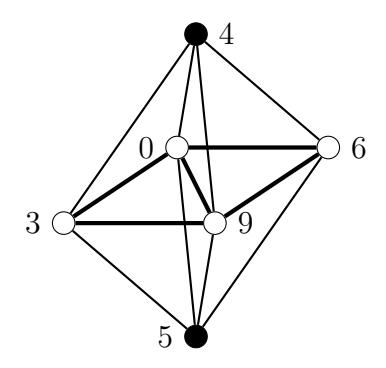
Figure 9. Harmonious labeling of \(G + 2K_1\), where G is strongly indexable.

5. Harmonious Disconnected Graphs

In [8], Graham and Sloane characterized the harmonious complete bipartite graphs. A complete bipartite graph is harmonious if and only if it is acyclic, in other terms, if it is a star \(K_{1,n}\). Consider the complete bipartite graph \(K_{m,n}\) where \(2 \le m \le n\). Since \(m \ge 2\), this graph contains at least one cycle, therefore it is not harmonious, however, \(K_{m,n} \cup K_2\) is harmonious. Note that when m=n=2, \(K_{2,2} \cup K_2\) is a disconnected unicyclic graph of order 6 and size 5, which means that any harmonious labeling of it must repeat one label. We show the harmonious labeling of this graph in Figure 10, in addition we show two more examples of the labeling described in the proof of the following proposition.

Proposition 5.1. For every \(2 \le m \le n\), the graph \(K_{m,n} \cup K_2\) is harmonious.

Proof. Let \(R=\{u_1,u_2,\ldots,u_m\}\) and \(S=\{v_1,v_2,\ldots,v_n\}\) be the stable sets of \(K_{m,n}\). Assign to the elements of R the labels \(0,1,\ldots,m-1\) and to the elements of S the labels \(m,2m,\ldots,nm\). Thus, the weights of the edges incident to \(v_j\) form the set \(W_j=\{jm-i+1,jm-i+2,\ldots,jm-1,jm\}\). Since \(j\in\{1,2,\ldots,n\},\bigcup_{j=1}^nW_j=\{m,m+1,\ldots,mn+m-1\}\). On the other side, the vertices of \(K_2\) are labeled with the integers m+1 and mn-1. In this way, the vertices of \(K_{m,n}\cup K_2\) are labeled with the integers \(0,1,\ldots,m+1,2m,3m,\ldots,nm\), and nm-1; i.e., with elements from \(\mathbb{Z}_{nm}\). The edge of \(K_2\) has weight mn+m. Then, the set of weights consists of mn+1 consecutive integers. Consequently, we have a harmonious labeling of the graph \(K_{n,m}\cup K_2\).

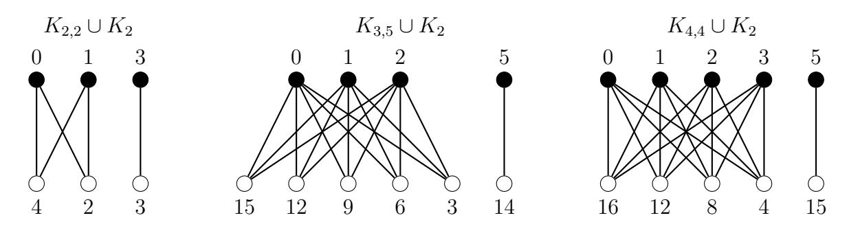
Figure 10. Harmoniously labeled graphs of the form Km,n ∪ K2.

We can go even further, as we prove in the following result.

Theorem 5.1. For every 2 ≤ m ≤ n, the graph Kn,m ∪ K1,m−¹ is harmonious .

Proof. We proceed as we did in Proposition 5.1. Thus, the vertices of R have labels 0, 1, . . . m−1; the vertices of S have labels m, 2m, . . . , nm. The vertex of degree m − 1 in K1,m−¹ is labeled nm − 1 and the leaves of K1,m−¹ receive the labels m + 1, m + 2, . . . , 2m − 1. In this way, the edges of this star have weights m(n + 1), m(n + 1) + 1, . . . , m(n + 1) + m − 2. Then, the weights on the edges of Km,n ∪ K1,m−¹ are mn + m − 1 consecutive integers, which implies that the graph is harmonious .

In Figure 11 we show an example of this labeling for the graph K4,⁴ ∪ K1,3.

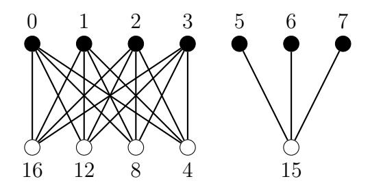
Figure 11. Harmoniously labeling of K4,⁴ ∪ K1,3.

Acknowledgement

We would like to thank the referee for his or her fine work and the valuable recommendations that certainly improve the quality of this work.

References

[1] C. Barrientos, On additive vertex labelings, Indonesian Journal of Combinatorics, 4(1) (2020), 34–52.

• [2] G. Chartrand and L. Lesniak, Graphs & Digraphs 4th ed. CRC Press (2005).
• [3] L.-C. Chen, On harmonious Labelings of the Amalgamation of Wheels, Masters Thesis, Chung Yuan Christian University, Taiwan.
• [4] R. Figueroa-Centeno, R. Ichishima, and F. Muntaner-Batle, Labeling the vertex amalgamation of graphs, Discuss. Math. Graph Theory, 23 (2003), 129–139.
• [5] J.A. Gallian, A dynamic survey of graph labeling, Electron. J. Combin. (2019), #DS6.
• [6] R.B. Gnanajothi, Topics in Graph Theory, Ph. D. Thesis, Madurai Kamaraj University, 1991.
• [7] T. Grace, On sequential labelings of graphs, J. Graph Theory, 7 (1983) 195–201.
• [8] R.L. Graham and N.J.A. Sloane, On additive bases and harmonious graphs, SIAM J. Alg. Discrete Methods, 1 (1980) 382–404.
• [9] B. Liu and X. Zhang, On harmonious labelings of graphs, Ars Combin., 36 (1993) 315–326.
• [10] S.C. Lopez and F.A. Muntaner-Batle, ´ Graceful, Harmonious and Magic Type Labelings: Relations and Techniques, Springer, Cham, 2017.
• [11] A. Kotzig, On certain vertex valuations of finite graphs, Util. Math., 4 (1973) 67–73.
• [12] A. Rosa, On certain valuations of the vertices of a graph, Theory of Graphs (Internat. Symposium, Rome, July 1966), Gordon and Breach, N. Y. and Dunod Paris (1967) 349–355.
• [13] P. Selvaraju and G. Sethurman, Decomposition of complete graphs and complete bipartitie graphs into copies of P 3 ⁿ or S2(P 3 n ) and harmonious labeling of K² + Pn, J. Indones. Math. Soc., Special Edition (2011) 109–122.
• [14] M.A. Seoud, A.E.I. Abdel Maqsoud, and J. Sheehan, Harmonious graphs, Util. Math., 47 (1995) 225–233.
• [15] M.A. Seoud and M.Z. Youssef, The effect of some operations on labeling of graphs, Proc. Math. Phys. Soc. Egypt, 73 (2000) 35–49.
• [16] S.C. Shee, On harmonious and related graphs, Ars Combin., 23 (1987) A, 237–247.
• [17] J. Yuan and W. Zhu, Some results on harmonious labelings of graphs, J. Zhengzhou Univ. Nat. Sci. Ed., 30 (1998) 7–12.
• [18] M.Z. Youssef, Note on even harmonious labeling of cycles, Util. Math., 100 (2016) 137–142.