Reza Sharafdini^a , Ali Zeydi Abdian^b

^aDepartment of Mathematics, Faculty of Intelligent Systems Engineering and Data Science, Persian Gulf University, Bushehr 75169, Iran

sharafdini@pgu.ac.ir azeydiabdi@gmail.com; aabdian67@gmail.com; abdian.al@fs.lu.ac.ir

A graph G is said to be determined by its Laplacian spectrum (DLS) if every graph with the same Laplacian spectrum is isomorphic to G. A graph which is a collection of hexagons (lengths of these cycles can be different) all sharing precisely one vertex is called a spinner graph. A tree with exactly one vertex of degree greater than 2 is called a starlike tree. If a spinner graph and a starlike tree are joined by merging their vertices of degree greater than 2, then the resulting graph is called a tarantula graph. It is known that spinner graphs and starlike trees are DLS. In this paper, we prove that tarantula graphs are determined by their Laplacian spectrum.

Keywords: tarantula graph, Laplacian matrix, Laplacian spectrum, L-cospectral

Mathematics Subject Classification : 05C50

DOI: 10.5614/ejgta.2021.9.2.14

1. Introduction

As usual G = (V (G), E(G)) is a simple graph having n = n(G) vertices and m = m(G) edges, with V (G) = {v1, v2, . . . , vn}. The complement of G is denoted by G. The degree sequence of G, denoted by deg(G), is the sequence of vertex degrees of G; in fact deg(G) = (d1, d2, . . . , dn)

Received: 08 November 2019, Revised: 23 March 2021, Accepted: 19 April 2021.

^bDepartment of Mathematical Sciences, Lorestan University, College of Science, Lorestan, Khoramabad, Iran

in which \(d_i = d_i(G) = d_G(v_i)\), for \(i = 1, \ldots, n\), is the degree of the vertex \(v_i\) so that \(d_1 \geq d_2 \geq \cdots \geq d_n\). For \(i = 0, 1, 2, \ldots, n-1\), let \(n_i = n_i(G)\) denote the number of vertices of degree i in G. Let A(G) and \(D(G) = \mathrm{Diag}(d_1, d_2, \ldots, d_n)\) denote the adjacency matrix and the diagonal matrix of vertex degrees of G, respectively. The Laplacian matrix of G is defined as L(G) = A(G) - D(G). The polynomial \(\varphi_{L(G)}(\mu) = \det(\mu \mathbb{I}_n - L(G))\), where \(\mathbb{I}_n\) is the identity matrix of order n, is called the Laplacian characteristic polynomial of G. Any root of \(\varphi_{L(G)}(\mu)\) is called a Laplacian eigenvalue of G. The multi-set of Laplacian eigenvalue of G is called the Laplacian spectrum or G. Note that the eigenvalues of G are all real non-negative, since it is a symmetric, positive semidefinite matrix. We denote its eigenvalues in the non-increasing order \(\mu_1 \geq \mu_2 \geq \cdots \geq \mu_n = 0\). The Laplacian matrix of G is a major tool for enumerating spanning trees of G and has numerous applications [18, 37]. Two graphs G and G is a said G-cospectral if they have the same G-spectrum, and a graph G is determined by its Laplacian spectrum, abbreviated by DLS, if no other graphs are G-cospectral with G. Only a few graphs with very special structures have been found to be determined by their spectra (DS, for short) (see [1]-[16], [19], [28]-[32], [34], [35] and the references cited therein).

The coalescence of two graphs \(G_1\) and \(G_2\), with respect to \(u_1 \in V(G_1)\) and \(u_2 \in V(G_1)\), is the graph obtained by identifying \(u_1\) and \(u_2\) in the disjoint union of \(G_1\) and \(G_2\). We denote it by \((G_1 \circ G_2)(u_1, u_2)\). In the case when it dose not make deference which vertex in \(G_1\) and \(G_2\) is identified to obtain a coalescence, we denote this graph by \(G_1 \circ G_2\). This operation is extended, inductively, to any arbitrary number of graphs. For instance, the coalescence of cycles \(C_{n_1}, \ldots, C_{n_p}\) (or \(C_{n_1} \circ \cdots \circ C_{n_a}\)) is called an a-rose graph. Specially, \(\text{[rumus tidak dapat ditampilkan dengan baik — lihat PDF asli]}\)

which is called an spinner graph and is denoted by \(H_a\).

An starlike tree is defined as a tree with a unique vertex v of degree greater than 2. We denote by \(S(t_1, \ldots, t_b)\) the starlike tree with maximum degree b such that

\[S(t_1,\ldots,t_b)-v=P_{t_1}\cup P_{t_2}\cup\cdots\cup P_{t_b},\]

where v is the vertex of degree b, and \(t_1, t_2, \ldots, t_b\) are any positive integers. We may describe an starlike tree as a coalescence of \(P_{t_1+1}, P_{t_2+1}, \ldots, P_{t_b+1}\). In fact, if \(v_i\) is a specific pendant vertex of \(P_{t_i+1}\), for \(i=1,\ldots,b\), then we have

\[S(t_1,\ldots,t_b) = P_{t_1+1} \circ P_{t_2+1} \circ \cdots \circ P_{t_b+1}(v_1,v_2,\ldots,v_b).\]

A tarantula graph, \(\mathfrak{T}(a,t_1,\ldots,t_b)\), \(a,b\geq 1\) is a graph of order \(n=5a+t_1+\cdots+t_b+1\), which consists of a hexagons and b paths of lengths \(t_1,t_2,\ldots,t_b\) sharing a common vertex. Note that \(\mathfrak{T}(a,t_1,\ldots,t_b)=H_a\circ T(u,v)\), where u and v are, respectively, the unique vertices of \(H_a\) and \(T=T_{t_1,t_2,\ldots,t_b}\) with the maximum degrees 2a and b, respectively, see Figure 1.

van Dam and Haemers [38] conjectured that almost all graphs are DLS. However, very few graphs are known to have that property, and so discovering new classes of such graphs is an interesting problem.

We are interested in DLS graphs being a coalescence of DLS graphs. Note that the coalescence of two DLS graphs is not, necessarily DLS, see Figure 2. All paths, cycles, starlike trees, triangle free 2-graph are DLS [26, 36, 41, 38]. In [24] it was shown that apart from two exceptional cases

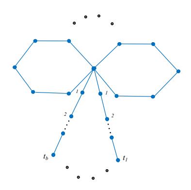
Figure 1. A tarantula graph \(\mathfrak{T}(a, t_1, \ldots, t_b)\)

of order 6 and 7, all roses are DLS. In [15] it was shown that \(\mathfrak{T}(2, 1, ..., 1)\) is DLS. In [40] it was shown that \(\mathfrak{T}(3, t_1)\) is DLS. In [35] it was shown that \(\mathfrak{T}(3, t_1, ..., t_b)\) is DLS.

Figure 2. Tow non-isomorphic graphs with the same Laplacian spectrum \(\{0, 3-\sqrt{5}, 2, 3, 3, 3+\sqrt{5}\}\), [39, 24]

The following theorem is our main result.

Theorem 1.1. All tarantula graphs and their complements are DLS.

The rest of this article is organized as follows: Section 2 contains preliminary results on the Laplacian spectrum of a graph, while Section 3 is devoted to the proof of Theorem 1.1.

2. Preliminaries

In this section, we recall some previously established results being used to prove Theorem 1.1. Note that the trace of a matrix M is denoted by tr(M).

Lemma 2.1. Let M and N be two matrices of size n. Then the following are equivalent:

• (i) M and N are cospectral;
• (ii) M and N have the same characteristic polynomial;
• (iii) \(\operatorname{tr}(M^i) = \operatorname{tr}(N^i)\) for i = 1, 2, ..., n.

Lemma 2.2 ([27, 34, 38, 42]). Let G be graph of size m with the Laplacian eigenvalues \(\mu_1 \ge \mu_2 \ge \cdots \ge \mu_n = 0\). Then the following hold:

• 1. the number of vertices of G is equal to n;
• 2. \(2m = \sum_{i=1}^{n} \mu_i\);
• 3. the number of spanning trees of G is equal to \(\prod_{i=1}^{n-1} \mu_i\);
• 4. the number of components of G is equal to the multiplicity of \(\mu_n = 0\);

5. \[\operatorname{tr}(L(G)^2) = \sum_{i=1}^n \mu_i^2 = 2m + \sum_{v \in V(G)} d_G^2(v)\].

The next lemma relates the Laplacian spectrum of a graph and its complements.

Lemma 2.3 ([20]). Let \(\mu_1 \ge \mu_2 \ge \cdots \ge \mu_n = 0\) and \(\overline{\mu}_1 \ge \overline{\mu}_2 \ge \cdots \ge \overline{\mu}_n = 0\) be the Laplacian spectrum of G and \(\overline{G}\), respectively. Then \(\overline{\mu}_i = n - \mu_{n-i}\) for \(i = 1, 2, \ldots, n-1\).

As a consequence of Lemma 2.3, we have the following fact:

Corollary 2.1. The complement of a DLS graph is also DLS.

Proof. Let G be a DLS graph and let H be a graph L-cospectral with \(\overline{G}\). Then it follows from Lemma 2.7 that \(\overline{H}\) is L-cospectral with G. Therefore, \(\overline{H} \cong G\), since G is DLS. Consequently, \(H \cong \overline{G}\), as desired.

We denote by \(\mathcal{N}_G(C_3)\) and \(\mathcal{W}_G(i)\), the number triangles of G, and the number of closed walks of length i in G, respectively.

The next lemma enables us to compute the number of closed walks of lengths 2, 3, and 4 in G:

Lemma 2.4 ([14, 42]). Let G be a graph with m edges. Then the following hold:

• 1. \(W_G(2) = 2m\);
• 2. \(W_G(3) = \operatorname{tr}(A^3(G)) = 6\mathcal{N}_G(C_3);\)
• 3. \(W_G(4) = 2m + 4\mathcal{N}_G(P_3) + 8\mathcal{N}_G(C_4)\).

Lemma 2.5 ([33]). Let G be a graph with n vertices and m edges, and let \(\varphi(G) = \sum_{i=1}^{n} l_i \mu^i\) be the Laplacian characteristic polynomial of G. Then

(i) \[l_0 = 1\], \(l_1 = -2m\), \(l_2 = 2m^2 - m - \frac{1}{2} \sum_{i=1}^n d_i^2(G)\);

(ii) \[l_3 = \frac{1}{3} \left( -4m^3 + 6m^2 + 3m \sum_{i=1}^n d_i^2(G) - \sum_{i=1}^n d_i^3(G) - 3 \sum_{i=1}^n d_i^2(G) + 6\mathcal{N}_G(C_3) \right).\]

It follows from Lemma 2.1 that L-cospectral graphs share the same characteristic polynomial. Hence the corresponding coefficients are also equal. Thus, the following lemma follows from the Lemma 2.5 and Lemma 2.4:

Lemma 2.6 ([26]). If G and H are two L-cospectral graphs, then

\[\operatorname{tr}(A^3(G)) - \sum_{i=1}^n (d_i^3(G) - 2)^3 = \operatorname{tr}(A^3(H)) - \sum_{i=1}^n (d_i^3(H) - 2)^3.\]

The following fact is a direct consequence of Lemma 2.4 and Lemma 2.6.

Corollary 2.2. Let G and H be L-cospectral graphs such that \(\deg(G) = \deg(H)\). Then \(\mathcal{N}_G(C_3) = \mathcal{N}_H(C_3)\).

Lemma 2.7 ([23]). Let G be a non-empty graph with n vertices. Then

\[\mu_1(G) \ge d_1(G) + 1.\] (1)

Furthermore, if G is connected, then the equality in (1) holds if and only if \(d_1(G) = n - 1\).

A graph G is called regular if \(d_1(G) = \cdots = d_n(G)\). A bipartite graph is called semi-regular if the degrees of vertices in each part, are constant.

For an arbitrary vertex u of G, we set \(\theta_G(u) = \sum_{v \in N_G(u)} \frac{d_G(v)}{d_G(u)}\), where \(N_G(u)\) denotes the set of neighbors of u in G.

Lemma 2.8 ([25, 27]). Let G be a connected graph. Then

\[\mu_1(G) \le \max_{u \in V(G)} d_G(u) + \theta_G(u),\]

with equality if and only if G is a regular or a semi-regular bipartite graph.

Lemma 2.9 ([14, 25]). If G is a non-empty graph, then \(\mu_1(G) \leq d_1(G) + d_2(G)\); and if G is connected, then \(\mu_2(G) \geq d_2(G)\).

Lemma 2.10 ([20]). Let \(\mu_1 \geq \mu_2 \geq \cdots \geq \mu_n\) be the eigenvalues of a symmetric \(n \times n\) matrix M, and let \(\lambda_1 \geq \lambda_2 \geq \cdots \geq \lambda_{n-1}\) be the eigenvalues of a principal sub-matrix of M of size n-1. Then \(\mu_1 \geq \lambda_1 \geq \mu_2 \geq \cdots \geq \mu_{n-1} \geq \lambda_{n-1} \geq \mu_n\).

Lemma 2.11 ([21]). Let G be a graph and \(\{u_1, u_2, \ldots, u_k, w_1, w_2, \ldots, w_p\} \subseteq V(G)\) such that

\[N_G(u_1) = N_G(u_2) = \dots = N_G(u_k) = \{w_1, w_2, \dots, w_p\}.\]

Let \(G^*\) be the graph obtained from G by adding q \((1 \le q \le {k \choose 2})\) edges among \(\{u_1, u_2, \ldots, u_k\}\). Then the eigenvalues of \(L(G^*)\) are as follows: those eigenvalues of L(G) being equal to p are incremented by \(\lambda_i(G^*[X])\), \(i=1,2,\ldots,k-1\), and the remaining eigenvalues are the same, where \(X=\{u_1,u_2,\ldots,u_k\}\).

Lemma 2.12 ([22]). No two non-isomorphic starlike trees are L-cospectral.

Note that in the proof of Lemma 2.12, the following observation was proved:

Lemma 2.13. If \(S_1 = S(l_1, \ldots, l_t)\) and \(S_2 = S(j_1, \ldots, j_t)\) are two non-isomorphic starlike trees, then \(\mu_1(S_1) \neq \mu_1(S_2)\), where \(l_1 \geq l_2 \geq \cdots \geq l_t \geq 1\) and \(j_1 \geq j_2 \geq \cdots \geq j_t \geq 1\).

3. Proof of Theorem 1.1

In this section, it is proved that all tarantula graphs are DLS. By an straightforward calculation we obtain the following fact:

Lemma 3.1. Let \(G = \mathfrak{T}(a, t_1, \dots, t_b)\) be a tarantula graph. Then

(i) \[n(G) = 5a + 1 + \sum_{i=1}^{b} t_i\], \(m(G) = n(G) + a - 1\);

(ii) \[\deg(G) = (2a+b, \underbrace{2, \dots, 2}_{n(G)-(b+1) \text{ times}}, \underbrace{1, \dots, 1}_{b \text{ times}}).\]

Lemma 3.2. If H is a graph L-cospectral with \(G = \mathfrak{T}(a, t_1, \dots, t_b)\), then

(i) \[2a + b + 1 \le \mu_1(H) \le 2a + b + 2\],

(ii) \[\mu_2(H) < 4\].

Proof. (i) By Lemma 2.7, \(\mu_1(G) \ge 2a + b + 1\), and by Lemma 2.8, \(\mu_1(G) \le 2a + b + 2\). This implies that \(2a + b + 1 \le \mu_1(H) = \mu_1(G) \le 2a + b + 2\).

(ii) Let v be the vertex with maximum degree of G, and let \(M_v\) be the \((n-1) \times (n-1)\) principal sub-matrix of L(G) formed by deleting the row and column corresponding to v. Since \(M_v\) contains negative entries, we consider \(|M_v|\) which is obtained by taking the absolute value of the entries of \(M_v\). Now \(M_v\) is reducible, but it has a+b irreducible sub-matrices that correspond to the components of G-v. On the other hand, each of these components has spectral radius strictly less than 4, so one can conclude that the largest eigenvalue of \(|M_v|\) is less than 4, and so is that of \(M_v\). By Lemma 2.10, \(\mu_2(G) < 4\) and so \(\mu_2(H) < 4\), as desired.

Theorem 3.1. If H is a graph being L-cospectral with \(G = \mathfrak{T}(a, t_1, \ldots, t_b)\), then they have the same degree sequence, i. e., \(\deg(H) = \deg(G)\), and \(\mathcal{N}_H(C_3) = 0\).

Proof. By Lemma 3.2(ii), \(\mu_2(H) < 4\), and thus it follows from Lemma 2.9 that \(d_2(H) \le 3\). Since H and G are L-cospectral, by Lemma 2.6, H is also connected, and has the same order, size, and sum of the squares of its degrees as G. Therefore, by Lemma 2.6, we have

\[\sum_{i=1}^{d_1(H)} n_i = n(G), \tag{2}\]

\[\sum_{i=1}^{d_1(H)} i n_i = 2m(G),\tag{3}\]

\[\sum_{i=1}^{d_1(H)} i^2 n_i = n_1(G) + 4n_2(G) + d_1^2(G), \tag{4}\]

Recall that by Lemma 3.1,

\[n(G) = 5a + 1 + \sum_{i=1}^{b} t_i, \quad m(G) = n(G) + a - 1,\]
\[n_1(G) = b, \quad n_2(G) = n(G) - (b+1),\]

and \(d_1(G) = 2a + b\). By adding (2), (3), and (4) with coefficients 2, -3, 1, respectively, we get:

\[\sum_{i=1}^{d_1(H)} (i^2 - 3i + 2)n_i(G) = 4a^2 + 4ab - 6a + (b-1)(b-2).\] (5)

By Lemma 3.1, \(\sum_{i=1}^{n} (d_i(G) - 2)^3 = ((2a + b - 2)^3 - b)\). Hence, it follows from Lemma 2.6 that

\[\mathcal{N}_H(C_3) = \frac{\sum_{i=1}^n (d_i(H) - 2)^3 - ((2a + b - 2)^3 - b)}{6}.\] (6)

By Lemma 3.2, \(2a+b+1 \le \mu_1(H) \le 2a+b+2\). It follows from Lemma 2.7 that \(d_1(H)+1 \le \mu_1(H) = \mu_1(G) \le 2a+b+2\), and so \(d_1(H) \le 2a+b+1\). Moreover, it follows from Lemma 3.2 and Lemma 2.9 that

\[2a + b + 1 \le \mu_1(G) = \mu_1(H) \le d_1(H) + d_2(H) \le d_1(H) + 3\]

which implies that \(d_1(H) \ge 2a + b - 2\). As a result, \(2a + b - 2 \le d_1(H) \le 2a + b + 1\). We claim that \(d_1(H) = 2a + b\). To prove our claim, we consider the following cases:

Case 1. \(d_1(H) = 2a + b + 1\)

Clearly, \(n_{2a+b+1} = 1\), since \(d_1(H) = 2a + b + 1 > 3 \ge d_2(H)\). From (5), we deduce that \(((2a+b+1)^2 - 3(2a+b+1) + 2) + 2n_3 = 4a^2 + 4ab - 6a + (b-1)(b-2).\)(7)

As a result, \(n_3 = -2a - b + 1 < 0\), which is impossible.

Case 2. \(d_1(H) = 2a + b\)

If b = 0, then for a = 1 we have \(H = C_6\) and in this case, the problem is clear, since cycles are DLS.

For \(a \ge 2\) and b = 0, we have

\[4a^2 - 6a + 2 + 2n_3 = 4a^2 - 6a + 2, (8)\]

which implies that \(n_3=0\). It follows from (2) and (3) that \(n_1=0\) and \(n_2=n-1\). Therefore, the degrees of H are the same as those of G and also \(d_1(H)=2a>3\geq d_2(H)\). If a=b=1, then \(d_1(H)=3\). By (5), \(n_3=1\). If \(a\neq 1\) or \(b\neq 1\), then \(d_1(H)=2a+b>3\geq d_2(H)\). As a result, for any natural numbers a,b we have \(n_{2a+b}=1\). Consequently, by (5) we have

\[((2a+b)^2 - 3(2a+b) + 2) + 2n_3 = 4a^2 + 4ab - 6a + b^2 - 3b + 2,\] (9)

from which we have \(n_3 = 0\). Combining (3) and (4), we obtain that \(n_1 = b\) and \(n_2 = n - (b+1)\). Therefore, \(\deg(H) = \deg(G)\). Hence, by Corollary 2.2, \(\mathcal{N}_H(C_3) = \mathcal{N}_G(C_3) = 0\).

Case 3. \(d_1(H) = 2a + b - 1\)

3.1. \(n_{2a+b-1}=1\).

In this case we have

\[((2a+b-1)^2 - 3(2a+b-1) + 2) + 2n_3 = 4a^2 + 4ab - 6a + (b-1)(b-2), (10)\]

Hence, \(n_3 = 2a + b - 2\). It follows from (3) and (4) that \(n_1 = 2a + 2b - 3\) and \(n_2 = n - 4a - 3b + 4\). Now, from (6) it is easy to see that

\[\mathcal{N}_H(C_3) = \frac{(2-b)(b-3) + (-4a^2 - 4ab + 10a)}{2}.\]

Let us prove that \(\mathcal{N}_H(C_3)<0\). To do so, assume that g(a,b)=-2a(2a+2b-5) and f(b)=(2-b)(b-3). It is easy to see that \(l(b)\geq 0\) if is either 2 or 3 and l(b)<0 otherwise. Therefore, for \(b\geq 3\), \(\mathcal{N}_H(C_3)=\frac{f(b)+g(a,b)}{2}<0\), which is impossible. Consequently, there are two subcases to be considered:

• 3.1.1. If b = 2, \(\mathcal{N}_H(C_3) = -2a^2 + a < 0\), which is impossible.
• 3.1.2. If b = 1, \(\mathcal{N}_H(C_3) = -2a^2 + 3a 1\). For \(a \ge 2\), \(\mathcal{N}_H(C_3) < 0\), which is impossible. For a = 1, \(n_{2a+b-1} = n_2 = 1\) and so by (5) we obtain that 2 = 0, which is impossible.
• 3.2 \(n_{2a+b-1} \geq 2\).

In this case we have

\[2a + b - 1 = d_1(H) = d_2(H) \le 3,\]

and so

\[(a,b) \in \left\{ (1,0), (1,1), (1,2) \right\}.\]

Consider the following subcases:

• 3.2.1. (a,b)=(1,2). In this case, \(d_1(H)=d_2(H)=3\). Hence, by (5) \(n_3=3\). Combining (3) and (4), we find that the roots are \(n_1=3\) and \(n_2=n-6\). It follows from (6) that \(\mathcal{N}_H(C_3)=-1\), a contradiction.
• 3.2.2. (a,b)=(1,1). In this case, \(d_1(H)=d_2(H)=2\). As before, we will have a contradiction.
• 3.2.3. (a,b)=(1,0). In this case, \(1=d_1(H)=d_2(H)\), and hence \(H=K_2\). But, (a,b)=(1,0) means that \(n(H)=n\geq 4\), a contradiction.

Case 4. \(d_1(H) = 2a + b - 2\)

4.1. \(n_{2a+b-2}=1\).

In this case,

\[2a + b - 2 = d_1(H) > 3 \ge d_2(H).\]

From (5), and by an straightforward calculation, we obtain that:

\[((2a+b-2)^2 - 3(2a+b-2) + 2) + 2n_3 = 4a^2 + 4ab - 6a + (b-1)(b-2).\](11)

As a result, \(n_3 = 4a + 2b - 5\). It follows from (3) and (4) that \(n_2 = n - 8a - 5b + 11\) and \(n_1 = 4a + 3b - 7\). Furthermore, by (6) \(\mathcal{N}_H(C_3) = -4a(a+b-3) - (b-3)^2\). We put

\[g(a,b) = -6a(a+b-3)\], and \(f(q) = -(b-3)^2\).

If \(b \ge 2\), then f(b) + g(a,b) < 0 and so \(\mathcal{N}_H(C_3) < 0\), a contradiction. So we need to consider the following cases:

• 4.1.1. b = 1. For \(a \ge 2\), \(\mathcal{N}_H(C_3) < 0\), which is impossible. If a = 1, then \(d_1(H) = 1 > 3\), which is impossible.
• 4.1.2. b = 0. Then f(0) + g(a, 0) < 0 and so \(\mathcal{N}_H(C_3) < 0\), a contradiction.
• 4.2. \(n_{2a+b-2} \geq 2\).

In this case,

\[d_1(H) = d_2(H) = 2a + b - 2 \le 3.\]

Hence

\[(a,b) \in \left\{ (0,1), (0,2), (1,1), (1,2), (2,1), (3,1) \right\}.\]

We have the following subcases:

• 4.2.1. (b,a)=(0,1). As a result \(d_1(H)=d_2(H)=0\), a contradiction, since H is connected.
• 4.2.2. (b, a) = (0, 2). So \(d_1(H) = d_2(H) = 2\) and so the degree sequence of H consists of either 1 or 2, which means that H is either a path or a cycle. Consequently, by (5) we get 0 = 6, which is impossible.
• 4.2.3. (b, a) = (1, 1). Obviously, \(n = n(H) \ge 6\). Moreover, \(1 = d_1(H) = d_2(H)\), which implies that \(H = K_2\), since H is a connected graph. This is clearly a contradiction.
• 4.2.4. (b,a)=(1,2). Therefore, \(3=d_1(H)=d_2(H)\). It follows from (2), (3) and (5) that \(n_1=4\), \(n_3=6\) and \(n_2=n-10\). Finally, it follows from (6) that \(\mathcal{N}_H(C_3)=-4\), which is impossible.
• 4.2.5. (b, a) = (2, 1). Therefore, \(2 = d_1(H) = d_2(H)\), a contradiction.
• 4.2.6. (b, a) = (3, 1). As a result, \(3 = d_1(H) = d_2(H)\). By (2), (3) and (4), we obtain that \(n_1 = n_3 = 6\) and \(n_2 = n 12\), which is impossible by (6).

Let x and y be, respectively, the unique vertices of \(G_1 = C_{k_1} \circ \cdots \circ C_{k_a}\) and \(G_2 = S(l_1, \ldots, l_b)\) with maximum degree; Consider \(G = G_1 \circ G_2(x, y)\) with maximum degree v. For each \(1 \le i \le a\), let \(e_i\) be an arbitrary edge of \(C_{k_i}\) being adjacent to v. Then \(G - \{e_1, \ldots, e_a\}\) is an starlike tree which is denoted by \(S_G\).

We are now ready to finalize the proof of Theorem 1.1. Let \(G = \mathfrak{T}(a, t_1, t_2, \dots, t_b)\) be a tarantula graph having a hexagons and b paths of lengths \(t_i\), \(i = 1, 2, \dots, b\). Assume that H is a graph L-cospectral with G. It follows from Theorem 3.1 that \(\deg(H) = \deg(G)\) and \(\mathcal{N}_H(C_3) = 0\).

Moreover, sine G is connected, it follows from Lemma 2.2 that H is also connected. Let v be the unique vertex of degree 2a+b in H. Then, H-v has maximum degree at most 2. We claim that H-v does not contain any cycles; otherwise, the connectedness of H implies that it must have another vertex of degree greater than 2, which is impossible. Consequently, H-v must be a forest each component of which is a path. Now due to the fact

\[d_H(v) = 2a + b\], \(\mathcal{N}_H(C_3) = 0\), \(n_1 = b\), \(\deg(H) = (2a + b, \underbrace{2, \dots, 2}_{n(G) - (b+1) \text{ times}}, \underbrace{1, \dots, 1}_{b \text{ times}})\)

we conclude that there exist natural numbers \(k_1, \ldots, k_a \geq 2\) such that

\[H \cong (C_{k_1} \circ C_{k_2} \circ \cdots \circ C_{k_a}) \circ S(t_1, \ldots, t_b)(x, y),\]

where x and y are, respectively, the unique vertices of \(C_{k_1} \circ \cdots \circ C_{k_a}\) and \(S(t_1, \ldots, t_b)\) with maximum degree; Consider starlike trees \(\mathcal{S}_G\) and \(\mathcal{S}_H\). It follows from Lemma 2.11 that \(\mu_1(\mathcal{S}_G) = \mu_1(G)\) and \(\mu_1(\mathcal{S}_H) = \mu_1(H)\), from which we have \(\mu_1(\mathcal{S}_G) = \mu_1(\mathcal{S}_H)\) since \(\mu_1(H) = \mu_1(G)\). Thus by Lemma 2.13, we have \(G \cong H\), which as direct consequence of Corollary 2.1, we have \(\overline{G} \cong \overline{H}\), as desired.

4. Conclusion

Let G be a tarantula graph. In this article, we show that tarantula graphs are determined by their Laplacian Spectrum (DLS) trough the fact that a graph which is L-cospectral with a tarantula graph is a triangle-free graph with the same vertex degree sequence as G.

Let us put forward the following questions for further research in the future:

Question 1. Are tarantula graphs determined by their adjacency spectrum (DAS)?

Question 2. Are tarantula graphs determined by their signless Laplacian spectrum (DQS)?

References

• [1] A.Z. Abdian, Graphs which are determined by their spectrum, Konuralp J. Math., 4 (2016), 34–41.
• [2] A.Z. Abdian, Two classes of multicone graphs determined by their spectra, J. Math. Ext., 10 (2016), 111–121.
• [3] A.Z. Abdian, A.R. Ashrafi and M. Brunetti, Signless Laplacian spectral characterization of roses, Kuwait j Science, 47 (2020), 12–18.
• [4] A.Z. Abdian, Graphs cospectral with multicone graphs \(K_w\nabla L(P)\), TWMS. J. App and Eng. Math. 7 (2017), 181–187.
• [5] A.Z. Abdian, The spectral determination of the multicone graphs \(K_w \nabla P\), arXiv preprint arXiv:1703.08728 (2017).

• [6] A.Z. Abdian, A. Behmaram, and G.H. Fath-Tabar, Graphs determined by signless Laplacian spectra, AKCE Int. J. Graphs Comb., 17 (2020), 45–50.
• [7] A.Z. Abdian and S.M. Mirafzal, On new classes of multicone graph determined by their spectrums, Alg. Struc. Appl. 2 (2015), 23–34.
• [8] A.Z. Abdian and S.M. Mirafzal, The spectral characterizations of the connected multicone graphs Kw∇LHS and Kw∇LGQ(3, 9), Discrete Math. Algorithms Appl. 10 (2018), 1850019.
• [9] A.Z. Abdian and S.M. Mirafzal, The spectral determinations of the connected multicone graphs Kw∇mP¹⁷ and Kw∇mS, Czech. Math. J. (2018), 1–14.
• [10] A.Z. Abdian, L.W. Beineke, M.R. Oboudi, A. Behmaram, K. Thulasiraman, S. Alikhani, and K. Zhao, On the spectral determinations of the connected multicone graphs Kr∇sK^t , AKCE Int. J. Graphs Comb., 17 (2020), 149–158.
• [11] A.Z. Abdian, L.W. Beineke, K. Thulasiraman, R. Tayebi Khorami, and M.R. Oboudi, The spectral determination of the connected multicone graphs Kw∇rCs, AKCE Int. J. Graphs Comb., https://doi.org/10.1080/09728600.2021.19.
• [12] A.Z. Abdian, K. Thulasiraman, and K. Zhao, The spectral characterization of the connected multicone graphs Kw∇mKn,n, AKCE Int. J. Graphs Comb., 17 (2020), 606–613.
• [13] A.Z. Abdian and M. Ziaie, Signless Laplacian spectral determinations of the starlike trees ST(n; d1) and the double starlike trees Hn(p; p), Ars Combinatorica, (2019), In press.
• [14] A.Z. Abdian, G.H. Fath-Tabar, and M. R. Moghaddam, The spectral determination of the multicone graphs Kw∇C with respect to their signless Laplacian spectra, J. Algebraic Systems, 7 (2) (2020), 131–141.
• [15] A.Z. Abdian, Bell graphs are determined by their Laplacian spectra, Kragujevac J. Math., (2023), 47, 203–211.
• [16] A.Z. Abdian and A.M. Moez, The spectral determinations of the join of two friendship graphs, Honam J. Math., (2019), 41, 67–87.
• [17] W.N. Anderson and T.D. Morley, Eigenvalues of the Laplacian of a graph, Linear Multilinear Algebra 18 (1985), 141–145.
• [18] N. Biggs, Algebraic Graph Theory, Cambridge University Press, Cambridge, 1993.
• [19] S. Pouyandeh, A.M. Moez, and A.Z. Abdian, The spectral determinations of connected multicone graphs K^w 5 mCP(n), Aims Mathematics 4, (2019), 1348–1356.
• [20] D. Cvetkovic, P. Rowlinson, and S. Simi ´ c,´ An Introduction to the Theory of Graph Spectra, London Mathematical Society Student Texts 75, Cambridge Univ. Press, Cambridge, 2010.

• [21] K.Ch. Das, The Laplacian sprectrum of a graph, Comput. and Appl. Math. 48 (2004), 715– 724.
• [22] L. Feng and G. Yu, No starlike trees are Laplacian cospectral, Univ. Beograd. Publ. Elektrotehn. Fak. Ser. Mat. 18 (2007), 46–51.
• [23] R. Grone and R. Merris, The Laplacian spectrum of graph II, SIAM J. Discrete Math. 7 (1994), 221–229.
• [24] C. He and E.R. van Dam, Laplacian spectral characterization of roses, Linear Algebra Appl. (2018), in press.
• [25] J.S. Li and Y.L. Pan, A note on the second largest eigenvalue of the Laplacian matrix of a graph, Linear and Multilinear Algebra 48 (2000), 117–121.
• [26] F.J. Liu and Q.X. Huang, Laplacian spectral characterization of 3-rose graphs, Linear Algebra Appl. 439 (2013), 2914–2920.
• [27] R. Merris, A note on the Laplacian graph eigenvalues, Linear Algebra Appl. 285 (1998), 33–35.
• [28] S.M. Mirafzal and A.Z. Abdian, Spectral characterization of new classes of multicone graphs, Studia. Univ. Babes¸-Bolyai Mathematica, 62 (2017), 275–286.
• [29] S.M. Mirafzal and A.Z. Abdian, The spectral determinations of some classes of multicone graphs, J. Discrete Math. Sci. Cryptogr. 21 (2018), 179–189.
• [30] R. Sharafdini, A.Z. Abdian, and A. Behmaram, Signless Laplacian determination of a family of double starlike trees, Ukrainian Mathematical Journal, In press.
• [31] R. Sharafdini and A.Z. Abdian, Signless Laplacian determination of path-friendship graphs, Acta Math. Univ. Comenianae, (2021), In press.
• [32] R. Sharafdini and A.Z. Abdian, Signless Laplacian determinations of some graphs with independent edges, Carpathian Math. Publ. 10 (2018), 185–191.
• [33] C.S. Oliveira, N.M.M. de Abreu, and S. Jurkiewilz, The characteristic polynomial of the Laplacian of graphs in (a,b)-linear cases., Linear Algebra Appl. 356 (2002), 113–121.
• [34] M.R. Oboudi, A.Z. Abdian, A.R. Ashrafi, and L.W. Beineke, Laplacian spectral determination of path-friendship graphs, Accepted in AKCE Int. J. Graphs Comb., (2021), doi: 10.1080/09728600.2021.1917321.
• [35] M.R. Oboudi and A.Z. Abdian, Peacock Graphs are Determined by Their Laplacian Spectra, Iran J. Sci. Technol. Trans. Sci. 44 (2020), 787–790.
• [36] G.R. Omidi and K. Tajbakhsh, Starlike trees are determined by their Laplacian spectrum, Linear Algebra Appl. 422 (2007), 654–658.

• [37] K.L. Patra and B.K. Sahoo, Bounds for the Laplacian spectral radius of graphs, Electron. J. Graph Theory Appl. 5 (2) (2017), 276–303.
• [38] E.R. van Dam and W.H. Haemers, Which graphs are determined by their spectrum?, Linear Algebra Appl. 373 (2003), 241–272.
• [39] E.R. van Dam, Graphs with Few Eigenvalues - An Interplay between Combinatorics and Algebra, thesis, Tilburg University, 1996; https://pure.uvt.nl/portal/files/193719/ Graphswi.pdf.
• [40] L. Wang and L. Wang, Laplacian spectral characterization of clover graphs, Linear Multilinear Algebra 63 (2015), 2396–2405.
• [41] J. Wang, Q. Huang, F. Belardo, and E.M. Li Marzi, On the spectral characterizations of ∞ graphs, Discrete Math. 310 (2010), 1845–1855.
• [42] F. Wen, Q. Huang, X. Huang, and F. Liu, The spectral characterization of wind-wheel graphs, Indian J. Pure Appl. Math. 46 (2015), 613–631.