Computer search for graceful-like labelling: A survey
Ljiljana Brankovic∗a , Michael J. Reynoldsb
aSchool of Science and Technology, University of New England, Australia
lbrankov@une.edu.au, m.reynolds@unsw.edu.au
This paper surveys the main computer search results for finding graceful labelling of trees. The paper is devoted to the memory of Mirka Miller, who made an outstanding contribution to the area of graph labelling.
Keywords: graph labelling, graceful labelling, graceful tree conjecture, computer search
Mathematics Subject Classification: 05C78
DOI: 10.5614/ejgta.2022.10.1.23
1. Introduction
Graph labellings are a relatively new area of graph theory that trace their origins back to Rosa's 1967 paper [44], in which he introduced four hierarchically related labellings, one of which is today known as 'graceful labelling', and showed their connection to the well know Ringel's conjecture [42], which states that the complete graph on 2n + 1 vertices can be decomposed into 2n + 1 subgraphs that are all isomorphic to a given tree with n edges. See also [9, 12, 21, 25, 30].
Since then, there have been over 1000 papers published on the topic, introducing new types of labelling or discovering new properties of old ones [5, 14, 15, 24, 38, 40, 41, 48, 45]. As many papers were published in journals that were not widely available [29], many of the papers have only 'rediscovered' the previously published results [36].
Received: 8 April 2020, Revised: 19 December 2020, Accepted: 2 October 2021.
bSchool of Mathematics and Statistics, University of New South Wales, Australia
∗Corresponding author
The most famous conjecture arising from these graph labellings is the so-called Graceful Tree Conjecture, which states that all trees have a graceful labelling. This conjecture have also been referred to as the Ringel-Kotzig, Rosa or Ringel-Kotzig-Rosa conjecture, and has been studied or referred to by many combinatorialists around the globe. For example, Erdos, Hell and Winkler ¨ state in their 1989 paper [26] that "the largest size of a numbering of G bears an obvious relation to graceful graphs; this notion, in some sense dual to the notion of bandsize of the graph, may be called the gracesize of G, gs(G). Because of the famous graceful tree conjecture, it could be interesting to prove nontrivial lower bounds on the gracesize of trees. . . ."
Graceful labelling is not only an interesting isolated problem but also has strong connections to many other problems in combinatorics and graph theory. It is relevant to some other types of labelling, i.e., edge antimagic vertex labelling [7], the Ringel conjecture [43], the Oberwolfach problem [32], map colouring and near-transversals in Latin squares [19, 37, 50]. Graceful labelling is related to cyclic difference sets, sequenceable groups, generalized complete mappings, nearcomplete mappings, and neofields [29, 22, 34, 35]. Graph labellings have been used as models for coding theory, x-ray crystallography, radar, astronomy, circuit design, communication network addressing, data base management, and models for constraint programming over finite domains [29].
2. Graceful and Graceful-Like Labellings
A graceful labelling of a finite undirected graph G = (V, E), is a one-to-one mapping f from the set V of vertices of G to the set {0, 1, 2, . . . , m}, where m = |E|, such that the induced edge labels are all distinct. Given f, an "induced edge labelling" is one-to-one mapping f ′ from the set of edges of G to the set {1, 2, . . . , m} given by f ′ (u, v) = |f(u) − f(v)|.
Example. Consider a cycle with 11 edges. If the consecutive vertices are labelled with numbers 0, 11, 1, 10, 2, 9, 4, 8, 5, 7, 6 then the edge labels are 11, 10, 9, 8, 7, 5, 4, 3, 2, 1, 6 (see Figure 1). In fact, Rosa [44] showed that all cycles with 4k or 4k − 1 edges, k ≥ 1, can be gracefully labelled in the same manner: Start from the smallest label (0), then use the largest (4k − 1), then the second smallest (1), then the second largest (4k − 2), and so on, until we reach the label k, which we skip and use k + 1 instead; we then continue in the same manner until all the vertices are labelled.
In his seminal paper from 1967 [44], Alex Rosa introduced the graceful labelling together with three related types of labellings, which he referred to as 'valuations'. He referred to graceful labelling as β-valuation, a special case of σ-valuation, which is in turn a special case of ρvaluation. On the other end of the spectrum, α-valuation is a special case of graceful labelling (i.e., β-valuation). The formal definitions of all 4 types of labellings are given bellow.
- 1. An α-labelling of a graph G with n vertices and m edges is a one-to-one mapping f from the set of vertices of G to the set {0, 1, 2, . . . , m} such that all induced edge labels are distinct, where the induced edge label of the edge uv is |f(u) − f(v)|, and such that there exists a number x ∈ {0, 1, 2, . . . , m} such that for an arbitrary edge uv either f(u) ≤ x < f(v) or f(v) ≤ x < f(u).
- 2. A β-labelling of a graph G with n vertices and m edges is a one-to-one mapping f from the set of vertices of G to the set {0, 1, 2, . . . , m} such that all induced edge labels are distinct. In 1972 Golomb independently introduced the same labelling and called it 'graceful'.
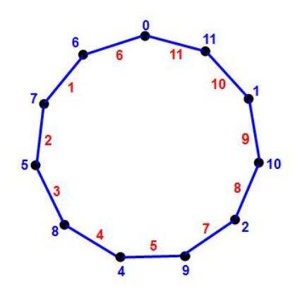
Figure 1. Graceful labelling of the 11-cycle. Note the (blue) vertex labels range from 0 to 11 and induce the (red) edge labels which give the integers 1, . . . , 11 distinctly.
- 3. A σ-labelling of a graph G with n vertices and m edges is a one-to-one mapping f from the set of vertices of G to the set {0, 1, 2, . . . , 2m} such that all induced edge labels are distinct and in the range {1, . . . , m}.
- 4. A ρ-labelling of a graph G with n vertices and m edges is a one-to-one mapping f from the set of vertices of G to the set {0, 1, 2, . . . , 2m} such that the set of induced edge labels is {x1, x2, . . . , xm}, where xi = i or xi = 2m + 1 − i.
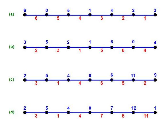
Figure 2. α, β, σ and ρ labellings of a path with 7 vertices
The four labellings defined above are illustrated in Figure 2 on a path with 7 vertices. The first labelling, shown in Figure 2 (a) shows an α-labelling. Note that an α-labelling can be seen as a "bipartite" graceful labelling, where bipartite labelling means that the vertex labels are partitioned
into two groups, say "small" and "large" labels, such that a vertex with a small label is connected only to vertices with large labels and vice versa. Figure 2 (b) illustrates β (graceful) labelling. Note that this labelling is not an α-labelling, as vertices labelled by 1 and 2 are adjacent. In σ-labelling in Figure 2 (c) vertex labels are drawn from the range {0, 1, 2, . . . , 12}, while edge labels are still from the range {1, . . . , 6}. Finally, ρ-labelling in Figure 2 (d) has the vertex labels in the same range as σ-labelling, while edge labels take exactly one value from each of the following pairs of labels: (1, 12),(2, 11),(3, 10),(4, 9),(5, 8) and (6, 7).
In what follows we will always start labelling vertices from 1 rather than from 0, that is, we will use {1, 2, . . . , m + 1} as the set of vertex labels, instead of {0, 1, . . . , m}.
3. Progress Towards the Graceful tree Conjecture
There are two main direction that have been taken in order to prove the Graceful Tree Conjecture.
The first direction is to consider different classes of trees and find graceful or graceful-like labelling for the class. There has been a large body of research in this direction which resulted in numerous publications. The drawback of this direction is that the classes of trees considered are typically very restricted and there are still no results for classes of trees such as trees with bounded degree. Therefore, the progress achieved in this direction is still very limited.
The second direction is to relax the requirement of graceful and graceful like labellings that all induced edge labels need to be distinct. To this end, we define a grace-size and an α-size of a labelled graph. In what follows a labelling of vertices of a graph is said to be "proper" if no two vertices receive the same label.
- 1. The grace-size of a graph is the maximum number of distinct edge labels taken over all proper labellings of the graph, where the labels are in the range [1, m + 1].
- 2. The α-size of a graph is the maximum number of distinct edge labels taken over all proper bipartite labellings of the graph where the labels are drawn from the range [1, m + 1].
A graph has a graceful labelling if and only if its grace-size (β-size) is equal to the number of edges m. Similarly, a graph has an α-labelling if and only if its α-size is equal to the number of edges m.
Proving nontrivial lower bounds for grace-size and α-size of a tree, and then "pushing" these bounds towards m is another way of attacking the Graceful Tree Conjecture. The advantage of this approach is that one can consider larger classes of trees, including trees with bounded degree.
In the rest of this section, we examine in detail the progress made in both of these directions.
3.1. Known Graceful Graphs
We next present the main classes of trees known to be graceful, and for each one of them we comment if they are known to have/not have an α-labelling.
3.1.1. Paths
Definition 3.1. A path is either a tree consisting of a single vertex or a tree in which all vertices have degree either 1 or 2. The length od a path is the number of its edges.
Paths were among the first trees to be found graceful.
Theorem 3.1. [44] All paths are graceful.
It is easy to see that all paths also have α-labelling.
Theorem 3.2. [44] Every path has an α-labelling.
It is easy to see that as the length of a path grows, the number of graceful and α-labelling that it admits grows very fast. The first bound on the number of graceful labellings of paths was established by Abraham and Kotzig [1].
Theorem 3.3. [1] The number of graceful labellings of the path Pn with n vertices grows asymptotically (for sufficiently large n) at least as fast as 1.39n .
This bound was improved by Aldred, J. Sir ˇ a´n and M. ˇ Sir ˇ a´n [4]. ˇ
Theorem 3.4. [4] The number of graceful labellings of the path Pn with n vertices grows asymptotically (for sufficiently large n) at least as fast as ( 5 3 ) n ≈ 1.67n .
As reported by Gallian [29], this bound was further improved by Adamaszek [2] as follows.
Theorem 3.5. [2] The number of graceful labellings of the path Pn grows asymptotically at least as fast as 2.37n .
3.1.2. Caterpillars
Definition 3.2. The base of a tree T is a tree obtained by deleting all the leaves of T.
Definition 3.3. A caterpillar is a tree whose base is a path.
Caterpillars are also among the trees Rosa considered in his 1967 paper [44].
Theorem 3.6. [44] Every caterpillar has an α-labelling.
Note that the above theorem implies that every caterpillar is graceful, as every α-labelling is also a graceful labelling.
Example. Consider a caterpillar shown in Figure 3. The labelling shown in the figure is an α-labelling. Note that all caterpillars can be labelled with α-labelling in the same manner.
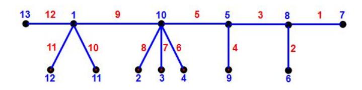
Figure 3. An α-labelling of a caterpillar
3.1.3. Lobsters
Definition 3.4. A lobster is a tree whose base is a caterpillar.
Bermond [9] conjectured that all lobsters are graceful.
Conjecture 1. [9] All lobsters are graceful.
Despite the limited progress [39, 49, 24], the above conjecture still remains open. Some classes of lobsters are known to be graceful, most notably the firecrackers.
Definition 3.5. A firecracker is a tree consisting of k − 1-path, k stars and k additional edges connecting each vertex on the path to the central vertex of a distinct star.
Theorem 3.7. [24] All firecrackers are graceful.
Example. Figure 4 shows a graceful labelling of a firecracker.
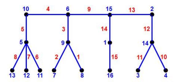
Figure 4. A graceful labelling of a firecracker
3.1.4. Banana Trees
Definition 3.6. A banana tree consists of a vertex v, k stars with at least one leaf and k additional edges connecting vertex v to one of the leaves of each star.
Chen, Lu and Yeh [24] conjectured that all banana trees are graceful.
Conjecture 2. [24] All banana trees are graceful.
The conjecture was recently proved by G. Sethuraman and J. Jesintha [47].
Theorem 3.8. [47] All banana trees are graceful.
3.1.5. Spiders
Definition 3.7. A spider is a tree with a root r and k paths ("legs") attached to the root.
It is still not known whether spiders are graceful. Some special cases of spiders are known to be graceful, as follows.
Definition 3.8. An olive tree is a spider with k legs, such that the length of leg i is i.
Theorem 3.9. [41] All olive trees are graceful.
Theorem 3.10. [8] Let T be a spider tree with k legs, each of which has length in {m, m + 1} for some m > 1. Then, T is graceful.
3.1.6. Symmetrical Trees
Definition 3.9. A symmetrical tree is a rooted tree in which all the vertices at the same distance from the root have the same degree.
Theorem 3.11. [11] All symmetrical trees are graceful.
3.1.7. Trees with Diameter less than 8
Theorem 3.12. [51] All trees with diameter less than 8 are graceful.
3.1.8. Trees with less than 5 leaves
Theorem 3.13. [44] All trees with less than 5 leaves are graceful.
We summarise the above results in the table below.
| Tree | α | graceful | ||
| Paths | Y | Y | ||
| Caterpillars | Y | Y | ||
| Lobsters | N | ?C | ||
| Special case: firecrackers | Y | Y | ||
| Bananas | ? | Y | ||
| Spiders | N | ? | ||
| Special case: Olive Trees | ? | Y | ||
| Symmetrical Trees | N | Y | ||
| < 8 Diameter | N | Y | ||
| < 5 end vertices | N | Y | ||
Table 1. Graceful Labelling: State of Art
3.2. Relaxed Labellings
While the graceful tree Conjecture states that all trees have a graceful labelling, it is easy to show that not all trees have an α-labelling. Alex Rosa [44] showed that the smallest tree that does not admit an α-labelling is the 2-star with 7 vertices (Figure 5). For convenience, in what follows we shall refer to this tree as the Y -tree. Note that it is easy to label the Y -tree gracefully, as shown in Figure 5.
Let α(n) be a minimum α-size over all trees with n vertices. Similarly, let α3(n) be a minimum α-size over all trees with n vertices and maximum degree 3, and let α PM 3 (n) be a minimum α-size over all trees with n vertices, maximum degree 3 and perfect matching.
The very first result on alpha-size of trees is due to Rosa and Sir ˇ a´n [46] who used mathematical ˇ induction to prove the following theorem.
Theorem 3.14. [46] The α-size of trees with n vertices satisfies 5n/7 ≤ α(n) ≤ (5n + 4)/6.
Figure 5. The Y-tree: the smallest tree without an \(\alpha\)-labelling.
Note that the \(\alpha\)-size of the Y-tree is 5, which is the lower bound on \(\alpha(7)\).
Bonnington and Širáň [16] considered trees with maximum degree 3 and for such trees with 12 or more vertices they were able to improve the above Rosa-Širáň's lower bound on \(\alpha\)-size to \(\alpha_3(n) \geq \frac{5n}{6}\). This result was further improved by Brankovic, Rosa and Širáň as follows.
Theorem 3.15. [18] The \(\alpha\)-size of trees with n vertices and maximum degree 3 satisfies \(\alpha_3(n) \ge \left\lfloor \frac{6n}{7} \right\rfloor - 1\).
Note that the equality is achieved for Y-tree.
Brankovic, Murch, Pond and Rosa [17] considered trees with and perfect matching, and showed that if all such trees have a graceful labelling, then all trees have a \(\sigma\)-labelling, which in turn would imply that the famous Ringel's conjecture holds. In particular, if all trees with maximum degree 3 and perfect matching have a graceful labelling, then all trees with maximum degree 3 have a \(\sigma\)-labelling. Therefore, it is well worthwhile considering the \(\alpha\)-size for trees with maximum degree 3 and perfect matching, denoted \(\alpha_3^{PM}\).
Theorem 3.16. [17] The \(\alpha\)-size of trees with n vertices, maximum degree 3 and perfect matching satisfies \(\alpha_3^{PM}(n) \ge \left\lceil \frac{14n}{15} \right\rceil - 1\).
Brinkman et. al [20] used computer search to find \(\alpha\)-size of all trees with up to 26 vertices, all trees with maximum degree 3 and at most 36 vertices, all trees with maximum degree 4 and at most 32 vertices, and all the tress with maximum degree 5 and at most 31 vertices.
In 2002 Van Bussel [48] generalised the concept of relaxed graceful and graceful-like labellings and defined the following three kinds of relaxed labellings for a graph with m edges:
- 1. Edge-relaxed graceful labelling where repeated edge labels are allowed.
- 2. Vertex-relaxed graceful labelling where repeated vertex labels are allowed.
- 3. Range-relaxed graceful labelling where there are more labels available for vertices than m + 1, and induced edge labels need only to be distinct and not necessarily in the range [1, m].
We have already discussed the edge-relaxed labellings, where the edge labels are not necessarily all distinct and we presented the best known bounds on the grace-size and the α-size of trees as a function of the number of vertices.
The only results on vertex-relaxed and range-relaxed labellings are as follows.
Theorem 3.17. [48] Every tree T on n vertices has a vertex relaxed graceful labelling such that the number of distinct vertex labels is strictly greater than n 2 .
Theorem 3.18. [48] Every tree T on n vertices has a range relaxed graceful labelling with vertex labels in the range 0 to 2m − diameter(T).
4. Computational Results
Several authors used computer search in order to find graceful and α labellings of trees. We here present the most important results.
4.1. Aldred-McKay's Algorithm
The first such result is due to Aldred and McKay [3] who showed that all trees with up to 27 vertices are graceful.The algorithm used for this search is a combination of hill climbing and tabu search.
Algorithm 1: Aldred-McKay algorithm for finding graceful labellings of trees
Input : Tree T = (V, E), labelling L of the vertices of T and a parameter M.
Output: Graceful labelling L of T.
In what follows α(T, L) denotes the number of distinct edge labels in the tree T with a vertex labelling L; SW AP(L; u, v) denotes the labelling obtained from L by swapping the labels on vertices u and v;
while α(T, L) < n − 1 do
   L0 = L;
   foreach pair {u, v} ∈ V do
       if α(T, SW AP(L; u, v)) > α(T, L) then
          L = SW AP(L; u, v);
   if L0 = L then
       Randomly select {u, v} ∈ V such that SW AP(L; u, v) is maximum over all pairs
       {u, v} that have not been chosen during the most recent M times this step has been
       executed;
The input to the algorithm is the tree to be labelled gracefully, as well as an initial labelling of the vertices of the tree and a tabu parameter M. The algorithm aims to maximise the number of distinct edge labels; it selects a vertex pair, say u and v, and swaps them if this leads to an increase in the number of distinct edge labels; otherwise the algorithm select another vertex pair and the
process continues. If no such pair exists, then the algorithm select a vertex pair {u, v} that has not been chosen in the last M steps and swaps them. The algorithm is given in Algorithm 1.
If it is not possible to further increase the number of distinct edge labels by the above method of swapping labels pairs of vertices (that is, when the algorithm "gets stuck"), the algorithm restarts with another randomly chosen labelling. The authors note that for smaller tree the value of M = 10 appears suitable, while a slightly bigger value should be used for larger trees. It appear advantageous to start the algorithm from a labelling close to a graceful labelling.
The above algorithm was used to label gracefully all the trees with up to 27 vertices.
4.2. Horton's Edge Search Algorithm
In 2003, Michael Horton [33] designed an Edge search algorithm for finding graceful labellings of trees, and used to gracefully label all trees with 29 vertices. Unlike the Aldred-McKay's algorithm, Horton's algorithm assigns labels to edges, rather than vertices. It is essentially a backtracking algorithm that initially selects an edge, say en−1, and assigns to it the largest label n−1, where n is the number of vertices in the tree. This implies that the labels on the edge end vertices are n and 1. The candidates for the second largest edge label n − 2 are the edges adjacent to en−1 such that the required label on the yet unlabelled end vertex is still available, that is, not equal to 1 and not equal to n. This process continues and if there are no candidates for the next edge label the algorithm backtracks.
It is important to note that Horton's algorithm is only able to discover graceful labellings with a property that each edge, except the edge labelled with the larger label n − 1, is adjacent to an edge labelled with a greater label. For example, the graceful labelling 2, 4, 3, 6, 1, 5 is a graceful labelling but cannot be obtained by the Edge search algorithm, as the edge with label 2 is only adjacent with the edge with a label 1 and not with any edge with a label greater than 2.
Conjecture 3. [33] All trees admit a graceful labelling where every edge label other than n-1 is adjacent to one edge of greater label.
Horton used the Edge search algorithm to verify the above conjecture on all trees with n ≤ 29 vertices.
4.2.1. Eshghi-Azimi's Mathematical Programming Algorithm
Eshghi and Azimi [27] used "nonzero" variables to model graceful labelling as a mathematical programming problem.
Graceful Labelling Problem
- 1. xi − xj = xij for all i, j, such that (vi , vj ) ∈ E(G);
- 2. xij − xkl = sijkl for all i, j, k, l, such that (i, j) ̸= (k, l) and (vi , vj ),(vk, vl) ∈ E(G);
- 3. xij + xkl = wijkl for all i, j, k, l, such that (i, j) ̸= (k, l) and (vi , vj ),(vk, vl) ∈ E(G);
- 4. xi − xj = yij for all i, j, such that i ̸= j, vi , vj ∈ V (G) and (vi , vj ) ∈/ E(G);
- 5. 0 ≤ xi ≤ m, integer, for all i such that vi ∈ V (G);
- 6. xij , sijkl, wijkl and yij are nonzero variables.
Eshghi and Azimi [27] developed a branch-and-bound algorithm for solving the above Graceful Labelling Problem and tested it on randomly generated graphs with up to 40 vertices.
4.3. Feng's Hybrid Algorithm
In 2010, Feng [28] proposed and implemented a hybrid algorithm consisting of 2 distinct parts: a deterministic backtracking algorithm and a probabilistic search similar to Aldred-McKay's algorithm based on hill climbing, tabu search and simulated annealing. In the first part, the number of backtracks is limited to an empirically determined value of 1000(n − 18). In the second part, the number of prohibited previously used swaps is set to ⌊ n 3 ⌋; this value has also been determined empirically. To each new tree given as an input, the algorithm first applies the deterministic backtracking, and if the graceful labelling is not found within the set time limit, the algorithm switches to probabilistic search.
Feng's Hybrid Algorithm has been run on all trees with up to 35 vertices, with a help from the Chinese community of volunteer computing.
Theorem 4.1. [28] All trees with up to 35 vertices are graceful.
4.4. Bonnington-Siran's Bipartite Labelling Algorithm
Bonnington and Siran [16] investigated α-labellings and edge relaxed α-labellings of trees with maximum degree 3 in order to determine their α-size. They designed a deterministic backtracking algorithm with branch pruning. Each node of a search tree corresponds to a partial bipartite labelling of the given tree, where the root of the search tree corresponds to an empty labelling while a leaf corresponds to a complete bipartite labelling. The set of all leaves therefore corresponds to the set of all bipartite labellings and the α-size can then be determined as the maximum number of distinct edge labels taken over all leaves of the search tree.
The branch pruning occurs when the number of repeated edge labels in an internal tree node equals or exceeds the number of repeated edge labels in some already obtained leaf. Additionally, algorithm makes use of the following fact: If two bipartite labellings L and L ′ satisfy the equation L ′ (u) = n − L(u) + 1 for every vertex u, then their induced edge labellings are identical.
The Bonnington-Siran's Bipartite Labelling Algorithm was run on all trees with maximum degree 3 with up to 17 vertices. The results of their search can be summarised in the following lemmas and Theorem.
Lemma 4.1. [16] There are exactly 5 trees with maximum degree three and order n ≤ 11 whose α-size equals n − 2. The α-size of all the remaining trees with maximum degree three of order n ≤ 11 is equal to n − 1.
Lemma 4.2. [16] There is exactly one tree with maximum degree three of order n = 12 and exactly one tree of order n = 15 whose α-size is equal to n − 2. Moreover, we have α3(n) = n − 2 if n = 12 or 15; α3(n) = n − 1 if n = 13 or 14, and n − 2 ≤ α3(n) ≤ n − 1 if n = 16 or 17.
Theorem 4.2. [16] For all n ≤ 17 we have n − 2 ≤ α ≤ n − 1.
The 7 exceptional trees that do not admit an α-labelling are shown in Figure 6.
Figure 6. The seven exceptional trees.
4.5. Brankovic-Murch-Pond-Rosa's Bipartite Labelling Algorithm for trees with maximum degree 3 and perfect matching
Brankovic, Murch, Pond and Rosa [17] used a hill climbing tabu search similar to that of Aldred and McKay to investigate \(\alpha\)-labellings of trees with maximum degree 3 and perfect matching. They run the algorithm on all such trees with up to 28 vertices and established that they all have an \(\alpha\)labelling.
Theorem 4.3. [17] For all n < 28 we have \(\alpha^{PM} = n - 1\).
The above computer search lead to the following result and conjecture on \(\alpha\)-size of trees with maximum degree 3 and perfect matching.
Theorem 4.4. [17] Let T be a tree with n vertices and with maximum degree three and perfect matching. Then \(\alpha(T) \ge \lfloor \frac{(k-1)n}{k} \rfloor - 1\), where 2k is the lower bound on the number of vertices of a tree with maximum degree three and perfect matching that does not admit an \(\alpha\)-labelling.
Conjecture 4. [17] All trees with maximum degree 3 and perfect matching have an \(\alpha\)-labelling.
5. Critical analysis of the previous computer search for graceful an \(\alpha\)-labelling
The previous computer searches presented in this section mostly focus on general trees and graceful labelling. Table 2 summarises the properties of these algorithms.
Table 2. Summary of Search Algorithms
| Algorithm | Type | Table 2. Summary of Search Algorithms Tree | Labelling | Tree | Outcome | Limitations |
|---|---|---|---|---|---|---|
| type | Type | Order | ||||
| Aldred- McKay | Hill Climbing Tabu Search | General Trees | Graceful | Up to 27 | All Graceful | |
| Horton | Backtracking | General Trees | Graceful | Up to 29 | All Graceful | Only finds labelling where each edge is adjacent to an edge with a larger label |
| Feng | Backtracking Hill Climbing Tabu Search Simulated Annealing | General Trees | Graceful | Up to 35 | All Graceful | |
| Bonnington- Siran | Backtracking | Trees with Max Degree 3 | α | Up to 17 | n − 2 ≤ α3 ≤ − n 1 | |
| Brankovic- Murch- Pond- Rosa | Hill Climbing Tabu Search | Trees with Max 3 Degree and Perfect Matching | α | Up to 28 | α All | |
| Brinkman- Crevals- Melot- Raylands- Steffan | Branch and Bound | General Trees 3 Trees with Max Deg 4 Trees with Max Deg 5 Trees with Max Deg | α | Up to 26 36 Up to 32 Up to 31 Up to | ≥ − α n 5 α ≥ n − 2 α ≥ n − 2 α ≥ n − 3 |
Some of these algorithms are rather efficient. However, due to the combinatorial explosion of the number of trees on n vertices as n grows larger, the best result today is limited to the trees of order 35 for general trees. Moreover, this result does not appear in a peer reviewed venue but was
rather self reported in http://arxiv.org/. Table 3 gives the number of unlabelled trees for a given n.
Table 3. Number of unlabelled trees of order n
| n | number of unlabelled trees | ||||
|---|---|---|---|---|---|
| 1 | 1 | ||||
| 2 | 1 | ||||
| 3 | 1 | ||||
| 4 | 2 | ||||
| 5 | 3 | ||||
| 6 | 6 | ||||
| 7 | 11 | ||||
| 8 | 23 | ||||
| 9 | 47 | ||||
| 10 | 106 | ||||
| 11 | 235 | ||||
| 12 | 551 | ||||
| 13 | 1,301 | ||||
| 14 | 3,159 | ||||
| 15 | 7,741 | ||||
| 16 | 19,320 | ||||
| 17 | 48,629 | ||||
| 18 | 123,867 | ||||
| 19 | 317,955 | ||||
| 20 | 823,065 | ||||
| 21 | 2,144,505 | ||||
| 22 | 5,623,756 | ||||
| 23 | 14,828,074 | ||||
| 24 | 39,299,897 | ||||
| 25 | 104,636,890 | ||||
| 26 | 279,793,450 | ||||
| 27 | 751,065,460 | ||||
| 28 | 2,023,443,032 | ||||
| 28 | 5,469,566,585 | ||||
| 30 | 14,830,871,802 | ||||
| 31 | 40,330,829,030 | ||||
| 32 | 109,972,410,221 | ||||
Therefore, it appears that we are reaching the limits of practically achievable searches by the above methods. On the other hand, in the area of α-labellings of trees with maximum degree 3 with a perfect matching and α-labellings, much improvement appears possible. The reason for this is twofold. First, α-labellings are more restricted and therefore easier to find than graceful labellings. Moreover, α-labellings can be readily combined to produce new α-labellings, which is not the case with graceful labellings. Secondly, trees with maximum degree 3 with a perfect
matching are on one hand a class sufficiently wide so that α-labellings for all such trees would imply the correctness of Ringel's conjecture for all trees with maximum degree 3 (see the next Section). On the other hand, this class of trees is sufficiently restricted to allow the search to go up to much higher number of vertices than for general trees.
References
References
- [1] J. Abrham and A. Kotzig, Exponential lower bounds for the number of graceful valuations of snakes, Congr. Numer. 72 (1990), 163–174.
- [2] M. Adamaszek, Efficient enumeration of graceful permutations, to appear in J. Combin. Math. Combin. Comput..
- [3] R.E. Aldred and B.D. McKay, Graceful and harmonious labellings of trees, Bull. Inst. Combin. Appl., 23, (1998), 69–72.
- [4] R.E. Aldred, J. Sir ˇ a´n, and M. ˇ Sir ˇ a´n, A Note on the number of graceful labelings of paths, ˇ Discrete Math., 261, (2003), 27–30.
- [5] M. Alfalayleh, L. Brankovic, H. Giggins, and Md. Z. Islam, Towards the graceful tree conjecture: a survey, AWOCA2004, 7-9 July, Ballina, Australia, (2004).
- [6] I. Arkut, R. Arkut, and N. Ghani, Graceful label numbering in optical MPLS networks, Proc. SPIE, 4233, (2000), 1–8, OptiComm 2000: Optical Networking and Communications, Imrich Chlamtac; Ed.
- [7] M. Baca and C. Barrientos, Graceful and edge-antimagic labelings, Ars Combin., to appear.
- [8] P. Bahl, S. Lake, and A. Wertheim, Gracefulness of families of spiders, Involve, 3(3), (2010) pp.241–247.
- [9] J.C. Bermond, Graceful graphs, radio antennae and french windmills, Graph Theory and Combinatorics, Pitman, London, (1979), 13–37.
- [10] J.C. Bermond, C. Huang, A. Rosa, and D. Sotteau, Decompositions of Complete Graphs into Isomorphic Subgraphs with Five Vertices, Ars Combinatoria 10, (1980), pp.211–254.
- [11] J.C. Bermond and D. Sotteau, Graph decompositions and G-designs, Cong. Numer., 15, (1976), 53–72. Sci.,
- [12] G.S. Bloom and S.W. Golomb, Applications of numbered undirected graphs, Proc. IEEE, 65, (1977) 562–570.
- [13] G.S. Bloom and S.W. Golomb, Numbered complete graphs, unusual rulers, and assorted applications, in Theory and Applications of Graphs, Lecture Notes in Math., 642, Springer-Verlag, New York, (1978), 53–65.
- [14] G.S. Bloom and D.F. Hsu, On graceful digraphs and a problem in network addressing, Congr. Numer., 35, (1982), 91–103.
- [15] G.S. Bloom and D.F. Hsu, On graceful directed graphs that are computational models of some algebraic systems, Graph Theory with Applications to Algorithms and Computers, Ed. Y. Alavi, Wiley, New York (1985).
- [16] C.P. Bonnington and J. Sir ˇ a´n, Bipartite labeling of trees with maximum degree three, ˇ J. Graph Th., 31, (1999), 37–56.
- [17] L. Brankovic, C. Murch, J. Pond, and A. Rosa. Alpha-size of trees with maximum degree three and perfect matching, Proceedings of AWOCA2005, 18–21 September, Ballarat, Australia, (2005), 47–56.
- [18] L. Brankovic, A. Rosa, and J. Sir ˇ a´n, Labeling of trees with maximum degree three an ˇ improved bound, J. Combin. Math. Combin. Comput., 55, (2005), 159–169.
- [19] L. Brankovic and I.M. Wanless, Graceful Labelling: State of the Art, Applications and Future Directions, Mathematics in Computer Science, 5(1), (2011), pp. 11–20.
- [20] G. Brinkmann, S. Crevals, H. Me`lot, L.J. Rylands, and E. Steffan, α-labelings and the structure of trees with nonzero α-deficit. Discrete Math. Theor. Comput. Sci., 14(1), (2012), 159– 174.
- [21] D. Bryant, Cycle Decomposition of Complete Graphs, Surveys in Combinatorics 2007, London Mathematical Society Lecture Note Series 34, (2007), pp. 67–97.
- [22] N.J. Cavenagh and I.M. Wanless, On the number of transversals in Cayley tables of cyclic groups, Disc. Appl. Math., 158, (2010), 136–146.
- [23] F.R.K. Chung and R.L. Graham, Recent results in graph decompositions, Combinatorics (Swansea, 1981), London Math. Soc. Lecture Note Ser. 52, Cambridge Univ. Press, Cambridge-New York, (1981), pp. 103–123.
- [24] W.C. Chen, H.I. Lu, and Y.N. Yeh, Operations of interlaced trees and graceful trees, Southeast Asian Bulletin of Mathematics, 21, (1997), 337–348.
- [25] D. Dor and M. Tarsi, Graph decomposition is NP-complete: A comlete proof of Holyer's conjecture, Siam J. Comput. 26, (1997), pp. 1166–1187.
- [26] P. Erdos, P. Hell, and P. Winkler, Bandwidth versus bandsize, ˝ Ann. Discrete Math., 41, (1989), 117–130.
- [27] K. Eshghi and P. Azimi, Applications of mathematical programming in graceful labeling of graphs, J. Appl. Math., 2004:1, (2004), 1–8.
- [28] W. Fang, A computational approach to the graceful tree conjecture, arXiv:1003.3045v1 [cs.DM]
- [29] J.A. Gallian, A dynamic survey of graph labeling, 20th edition, Electron. J. Combin., DS6, (2017).
- [30] L. Goddyn, R.B. Richter, and J. Sir ˇ a´n, Triangular embeddings of complete graphs from grace- ˇ ful labellings of paths, J. Combin. Theory Ser. B, 97, (2007), 964–970.
- [31] S.W. Golomb, How to number a graph, Graph Theory and Computing, R. C. Read, Academic Press, New York, (1972), 23–37.
- [32] P. Gvozdjak, On the Oberwolfach problem for cycles with multiple lengths, PhD Thesis, Simon Fraser University, (1993).
- [33] M. Horton, Graceful trees: Statistics and Algorithms, Honours thesis, University of Tasmania, (2003).
- [34] D.F. Hsu and A.D. Keedwell, Generalized complete mappings, neofields, sequenceable groups and block designs I, Pacific J. Math., 111, (1984), 317–332.
- [35] D.F. Hsu and A.D. Keedwell, Generalized complete mappings, neofields, sequenceable groups and block designs II, Pacific J. Math., 117, 1985, 291–312.
- [36] C. Huang, A. Kotzig, and A. Rosa, Further results on tree labellings, Util. Math., 21C, (1982), 31–48.
- [37] B.D. McKay, J.C. McLeod and I.M. Wanless, The number of transversals in a latin square, Des. Codes Cryptogr., 40, (2006), 269–284.
- [38] D. Morgan and R. Rees, Using Skolem and hooked-Skolem sequences to generate graceful trees, J. Combin. Math. Combin. Comput., 44, (2003), 47–63.
- [39] H.K. Ng, Gracefulness of a class of lobsters, Notices AMS, 7, (1986), 825–294.
- [40] Z. Nikoloski, N. Deo, and F. Suraweera, Generation of graceful trees, Congr. Numer., 157, (2002), 191–201.
- [41] A.M. Pastel and H. Raynaud. Les oliviers sont gracieux, Colloq. Grenoble, Publications Universite de Grenoble ´ , (1978).
- [42] G. Ringel, Problem 25, Theory of Graphs and its Application (Proc. Sympos. Smolenice 1963, Nakl. CSAV, Praha, 1964), 162, (1963).
- [43] G. Ringel, Map Color Theorem, Springer, 1974.
- [44] A. Rosa, On certain valuations of the vertices of a graph, Theory of Graphs, (Proc. Internat. Symposium, Rome, 1966), Gordon and Breach, N. Y. and Dunod Paris, (1967) 349–355.
- [45] A. Rosa, Labelling snakes, Ars Comb., 3, (1977), pp.67–74.
- [46] A. Rosa and J. Sir ˇ a´n, Bipartite labelings of trees and the gracesize, ˇ J. Graph Th., 19, (1995), pp.201–215.
- [47] G. Sethuraman and J. Jesintha, All banana trees are graceful, Advances and Applications Disc. Math., 4, (2009) pp.53–64.
- [48] F. Van Bussel, Relaxed graceful labellings of trees, Electron. J Combin., 9(1), (2002), R4.
- [49] J.G. Wang, D.J. Jin, X.G. Lu, and D. Zhang, The gracefulness of a class of lobster trees, Mathematical Computer Modelling, 20, (1994), 105–110.
- [50] I.M. Wanless, Transversals in latin squares, Quasigroups Related Systems, 15, (2007), 169– 190.
- [51] T.M. Wang, C.C. Yang, L.H. Hsu, and E. Cheng, Infinitely many equivalent versions of the graceful tree conjecture, Appl. Anal. Discrete Math., 9(1), (2015), 1–12.