Christina Eubanks-Turner^∗a , Kathryn Cole^b , Megan Lee^c

Loyola Marymount University, Los Angeles, CA, USA

ceturner@lmu.edu, kathryncole@ku.edu, leemeganh@gmail.com

In this paper, we examine interlace polynomials of lollipop and tadpole graphs. The lollipop and tadpole graphs are similar in that they both include a path attached to a graph by a single vertex. In this paper we give both explicit and recursive formulas for each graph, which extends the work of Arratia, Bollobas and Sorkin [4],[5], among others. We also give special values, examine adjacency ´ matrices and behavior of coefficients of these polynomials.

Keywords: graph polynomial, interlace polynomial, lollipop graph Mathematics Subject Classification: 05C31, 05C50, 11B39

DOI: 10.5614/ejgta.2022.10.1.14

1. Introduction

The interlace polynomial of a graph was introduced by Arratia, Bollobas, and Sorkin, and it ´ is a polynomial that contains and represents the information gained from performing the toggling process on the graph, see [4]. Interlace polynomials share similarities with other graph polynomials, such as Tutte and Martin polynomials as they are utilized in applications to science and other

Received: 14 December 2020, Revised: 22 December 2021, Accepted: 3 March 2022.

^aDepartment of Mathematics,

^bDepartment of Mathematics, University of Kansas, Lawrence, KS, USA

^cLos Angeles, CA, USA

^∗ corresponding author

fields, [6, 8, 10, 15]. More recently, researchers have studied different types of graph polynomials, such as Hosoya and M-polynomials, which give information about distance-based invariants related to chemical graphs,[1, 12, 9].

Interlace polynomials give important information about the graph, such as, the number of kcomponent circuit partitions, for k ∈ N. In [5], interlace polynomials for some simple graphs like paths, cycles, and complete graphs are given, although not all of the formulas are easy to use. Li, Wu and Nomani give recursive formulas for interlace polynomials of ladder and n-Claw graphs, see [13, 16]. In addition, Eubanks-Turner and Li give recursive and explicit formulas for friendship graphs, see [11]. Also, work has been done in utilizing bivariate and multi-variate interlace polynomials, see [3, 5, 18]. Here, we focus our attention on establishing the interlace polynomials of lollipop and tadpole graphs. Both graphs have the structure that each has a wellknown subgraph which is connected to a path by a single vertex.

A lollipop graph is a simple graph that consists of a complete graph being joined to a path with a bridge. Lollipop graphs have applications to stochastic processes and spectral graph theory [14, 19]. In particular, lollipop graphs have maximum possible hitting time, cover time and commute time [17]. In this work we consider the interlace polynomial of the lollipop graph. We give both the recursive and explicit formulas for the interlace polynomials of lollipop graphs. As Eubanks-Turner and Li did in [11], we consider natural questions regarding interlace polynomials of the lollipop graph, such as:

• 1. What are the general forms of the coefficients of the interlace polynomial of a lollipop graph?
• 2. What are the evaluations of the interlace polynomial of a lollipop graph at certain values and what does it describe about related graph properties?

We further consider graphs related to lollipop graphs called tadpole graphs. Tadpole graphs are simple graphs obtained by joining a cycle to a path via a bridge, [9]. Although the recursive and explicit formulas for interlace polynomials of tadpole graphs are given in [2], we give a different explicit formula and further results about interlace polynomials of tadpole graphs related to the latter mentioned questions.

For a simple graph G, to construct the interlace polynomial we first need the following definition. Note, ∀a ∈ V (G), N(a) = {neighbors of a}.

Definition 1.1. (Pivot) Let G = (V (G), E(G)) be any undirected graph without a loop and a, b ∈ V (G) with ab ∈ E(G). We first partition the neighbors of a or b into three classes:

• 1. N(a) \ ({b} ∪ N(b));
• 2. N(b) \ ({a} ∪ N(a));
• 3. N(a) ∩ N(b).

The pivot graph Gab of G, with respect to ab is the resulting graph of the toggling process: ∀u, v ∈ V (G), if u, v are from different classes shown above, then uv ∈ E(G) ⇐⇒ uv /∈ E(Gab).

Note that Gab = Gba. The pivot operation is only defined for an edge of G. The definition for the interlace polynomial of a simple graph G is given below. Here, ∀u ∈ V (G), G − u is the graph resulting from removing u and all the edges of G incident to u from G.

Definition 1.2. Let G be the class of finite undirected graphs having no loops nor multiple edges. There is a unique map \(q: G \to \mathbb{Z}[x]\), suhc that, \(G \mapsto q(G)\). For any undirected graph G with n vertices that has no loops nor multiple edges, the interlace polynomial q(G) of G is defined by

\[q(G) = \begin{cases} x^n, & \text{if } E(G) = \emptyset, \\ q(G-a) + q(G^{ab} - b), & \text{if } ab \in E(G). \end{cases}\]

This map is a well-defined polynomial on all simple graphs, see [2]. Next, we give some known results about interlace polynomials and results relating the interlace polynomials to structural components of graphs.

This map is a well-defined polynomial on all simple graphs, see [2]. Next, we give some known results about interlace polynomials and results relating the interlace polynomials to structural components of graphs.

Lemma 1.1. [5] Given the interlace polynomial q(G) of any undirected graph G, the following results hold:

• 1. The interlace polynomial of any simple graph has zero constant term.
• 2. For any two disjoint graphs \(G_1\), \(G_2\), we have \(q(G_1 \cup G_2) = q(G_1) \cdot q(G_2)\).
• 3. The degree of the lowest-degree term of q(G) is k(G), the number of components of G.
• 4. \(\deg(q(G)) \ge \alpha(G)\), where \(\alpha(G)\) is the independence number, i.e., the size of a maximum independent set.
• 5. Let \(\mu(G)\) denote the size of a maximum matching (maximum set of independent edges) in a graph G. If G is a forest with n vertices, then \(\deg(q(G)) = n \mu(G)\).

Lemma 1.2. [5] The interlace polynomials for the following graphs are as follows:

• 1. (complete graph \(K_m\)) \(q(K_m) = 2^{m-1}x\);
• 2. (complete bipartite graph \(K_{mn}\)) \(q(K_{mn}) = (1 + x + ... + x^{m-1})(1 + x + ... + x^{n-1}) + x^m + x^n 1;\)
• 3. (path \(P_n\) with n edges) \(q(P_1) = 2x\), \(q(P_2) = x^2 + 2x\), and for \(n \ge 3\), \(q(P_n) = q(P_{n-1}) + xq(P_{n-2})\);
• 4. (small cycles \(C_m\)) \(q(C_3) = 4x\) and \(q(C_4) = 2x + 3x^2\).

Definition 1.3. Let \(m, n \in \mathbb{N}\), with \(m \geq 3, n \geq 0\). The lollipop graph \(L_{m,n}\) is the simple graph obtained by joining a complete graph \(K_m\) to a path graph \(P_n\) at one of the vertices of \(K_m\). The lollipop graph \(L_{m,n}\) has m + n vertices and \(\binom{m}{2} + n\) edges. Note, we hold \(m \geq 3\) to disregard the case when \(L_{m,n}\) is a path.

2. Interlace Polynomial of Lollipop Graphs

Next, we develop interlace polynomials of lollipop graphs \(L_{m,n}\), where \(m, n \in \mathbb{N}\). We treat \(L_{m,0}\) as the complete graph with m vertices. The lollipop graph has the same recursive formula as the path graph, see Lemma 1.2 (3).

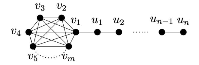
Figure 1. The graph Lm,n.

Lemma 2.1. Let m ≥ 3. For n ≥ 2, q(Lm,n) = q(Lm,n−1)+xq(Lm,n−2), where q(Lm,0) = q(Km) and q(Lm,1) = q(Km) + xq(Km−1).

Proof. Clearly, q(Lm,0) = q(Km).

Also, Lm,¹ is a graph consisting of a complete graph with m vertices and a path of length one. Labeling the edge of the path as ab, where deg(a) = 1, we have, q(Lm,¹ − a) = q(Km). Also note that L ab m,¹ − b = Km−¹ ∪ {a}, where b ∈ V (Km). So, q(Lm,1) = q(Km) + x · q(Km−1), by Lemma 1.2 (2).

Now assume n ≥ 2 and consider the graph Lm,n with the edge ab, such that deg(a) = 1. See the following figure.

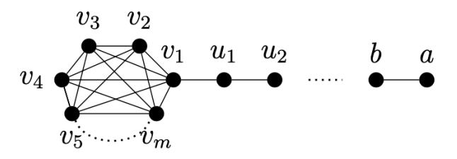
Figure 2. Lm,n.

Considering the interlace polynomial, we have that Lm,n − a = Lm,n−1.

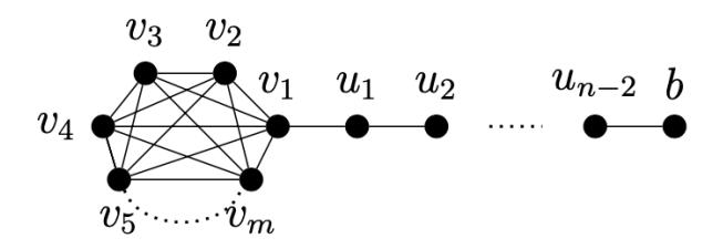
Figure 3. Lm,n − a.

Now toggling the graph, we have, L ab m,n − b = Lm,n−² ∪ {a}, as illustrated in the following figure, where n ≥ 2.

Interlace polynomials of lollipop and tadpole graphs | Eubanks-Turner et al.

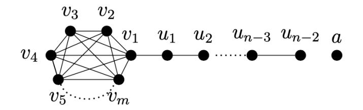
Figure 4. \(L_{m,n}^{ab} - b\).

Hence, \[q(L_{m,n}) = q(L_{m,n-1}) + xq(L_{m,n-2})\], for \(n \ge 2\) as desired.

The next result gives the explicit formula for the interlace polynomial of \(L_{m,n}\) for \(m \geq 3\) and \(n \geq 0\).

Theorem 2.1. For \(m \geq 3\) and \(n \geq 0\),

\[q(L_{m,n}) = \frac{1}{\sqrt{1+4x}} \left[ \frac{q(K_m) + \gamma x q(K_{m-1})}{\gamma^{n+1}} - \frac{(q(K_m) + \beta x q(K_{m-1}))}{\beta^{n+1}} \right]\]

where \[\gamma = \frac{\sqrt{1+4x}-1}{2x}\] and \(\beta = \frac{-\sqrt{1+4x}-1}{2x}\).

Proof. We utilize the recurrence relation in a generating function G(y), where the coefficient of \(y^n\) is \(q(L_{m,n})\):

\[G(y) = \sum_{n=0}^{\infty} q(L_{m,n}) y^n\]

By Lemma 2.1,

\[G(y) = q(L_{m,0}) + y \cdot q(L_{m,1}) + \sum_{n=2}^{\infty} (q(L_{m,n-1}) + xq(L_{m,n-2})) y^n\]\[= \frac{q(L_{m,0}) + y \cdot q(L_{m,1}) - y \cdot q(L_{m,0})}{1 - y - xy^2}\]

For convenience, let \(\gamma=\frac{\sqrt{1+4x}-1}{2x}\) and \(\beta=\frac{-\sqrt{1+4x}-1}{2x}\), the roots of the polynomial \(1-y-xy^2\). Since \(q(L_{m,0})=q(K_m)\) and \(q(L_{m,1})=q(K_m)+xq(K_{m-1})\), we have the desired result.

Proposition 2.1. For \(m \geq 3\), \(n \geq 0\), \(\deg(q(L_{m,n})) = 1 + \lceil \frac{n}{2} \rceil\), where \(1 + \lceil \frac{n}{2} \rceil = \alpha(L_{m,n})\), the independence number of \(L_{m,n}\).

Proof. The maximal independent set of vertices consists of the leaf, alternating non-adjacent vertices of the path, and potentially one vertex in the complete component of the graph. For even path length (n odd), this set is of size \(1 + \frac{n+1}{2}\). For odd path length (n even), it is size \(1 + \frac{n}{2}\). Including any additional vertex of the graph would result in a dependent vertex set. Therefore we have the desired result.

For paths of odd length, there are an even number of vertices, and at most \(\frac{n+1}{2}\) independent vertices. For paths of even length, there are an odd number of vertices, and at most \(\frac{n}{2}\) independent vertices. We have that \(\deg(q(L_{m,n})) = 1 + \left\lceil \frac{n}{2} \right\rceil\) by strong induction.

Arritia, Bollóbas and Sorkin evaluate interlace polynomials at certain small values of x, as these values give information relating to circuit partitions of the graphs, see [5]. They show that for any graph G, \(q(G)(2) = 2^{|V(G)|}\) and if H is the interlace graph of an Euler circuit of a 2-in, 2-out digraph D, then q(H)(1) is the number of Euler circuits of D.

We now give some propositions which show the evaluations of the lollipop graph at 1 and -1. In [5], the following corollary was given.

Corollary 2.1. [5] For the path \(P_n\), \(q(P_n)(1) = F_{n+2}\), the (n+2)'nd Fibonacci number (with \(F_0 = 0\) and \(F_1 = 1\)).

Since the lollipop has the same recursive formula as the path, we obtain similar results when evaluating at x = 1. For the evaluation at x = -1, we give our results in the same form as what was given in [2].

Proposition 2.2. For \(m \geq 3\), \(n \geq 0\),

1. \[q(L_{m,n})(1) = 2^{m-2}F_{n+3}\], the \((n+2)\)'nd Fibonacci number (with \(F_0 = 0\) and \(F_1 = 1\)).

2. \[q(L_{m,n})(-1) = \begin{cases} -2^{m-1}, & \text{if } n \equiv 0 \mod 6, \\ -2^{m-2}, & \text{if } n \equiv 1, 5 \mod 6, \\ 2^{m-2}, & \text{if } n \equiv 2, 4 \mod 6, \\ 2^{m-1}, & \text{if } n \equiv 3 \mod 6. \end{cases}\]

Proof. We prove (1) by strong induction on n. Note, \(q(L_{m,0})(1) = q(K_m)(1) = 2^{m-1} = 2^{m-2}F_3\), by Lemma 1.2 (1). Let \(n \ge 1\) and assume \(q(L_{m,n})(1) = 2^{m-2}(F_{k+3})\), for all \(k, 0 \le k \le n\). By Lemma 2.1,

\[\begin{array}{lll} q(L_{m,n+1})(1) & = & q(L_{m,n})(1) + q(L_{m,n-1})(1) \\ & = & 2^{m-2}(F_{n+3}) + 2^{m-2}(F_{n+2}) \\ & = & 2^{m-2}(F_{n+3} + F_{n+2}) \\ & = & 2^{m-2}(F_{n+4}), \text{ by definition of the Fibonacci sequence,} \\ & = & 2^{m-2}(F_{(n+1)+3}). \end{array}\]

For (2), also by Lemma 2.1,

\[q(L_{m,n})(-1) = q(L_{m,n-1})(-1) - q(L_{m,n-2})(-1)\] \[= [q(L_{m,n-2})(-1) - q(L_{m,n-3})(-1)] - q(L_{m,n-2})(-1)\] \[= -q(L_{m,n-3})(-1)\] \[= -q(L_{m,n-4})(-1) + q(L_{m,n-5})(-1)\] \[= -q(L_{m,n-5})(-1) + q(L_{m,n-6})(-1) + q(L_{m,n-5})(-1)\] \[= q(L_{m,n-6})(-1).\]

Therefore, \(q(L_{m,n})(-1)\) is periodic of period 6. The first six values of \(q(L_{m,n})(-1)\) are: \(q(L_{m,0})(-1) = -2^{m-1}\), \(q(L_{m,1})(-1) = -2^{m-2} = q(L_{m,5})(-1)\), \(q(L_{m,2})(-1) = 2^{m-2} = q(L_{m,4})(-1)\), \(q(L_{m,3})(-1) = 2^{m-1}\).

In the following Theorem Balister, Bollóbas, Cutler and Peabody give an explicit formula for the interlace at x = -1, therefore proving the conjecture in [7].

Theorem 2.2. [7] Let A be the adjacency matrix of G, n = |V(G)| and let r = rank(A + I) over \(\mathbb{Z}_2\) and I be the \(n \times n\) identity matrix. Then

\[q(G,-1) = (-1)^n (-2)^{n-r}.\]

Now we consider applications of lollipop graphs in solving a linear algebra problem. We determine the ranks of the adjacency matrices related to \(L_{m,n}\) over \(\mathbb{Z}_2\). For \(m \geq 3\), \(n \geq 0\), let \(A_{m,n}\) denote the adjacency matrix of \(L_{m,n}\). Then \(A_{m,n}\) has the form

\[\text{[rumus tidak dapat ditampilkan dengan baik — lihat PDF asli]}\]

with \[A_{m \times n} = [a_{ij}]\], where \(a_{ij} = \begin{cases} 1, & \text{if } j = i+1 \text{ or } j = i-1, \\ 0, & \text{otherwise.} \end{cases}\)

Proposition 2.3. Suppose \(m \ge 3\), \(n \ge 0\), let \(C_{m,n} = A_{m,n} + I_{m+n}\), where \(I_{m+n}\) is the \((m+n) \times (m+n)\) identity matrix. Then, \(rank(C_{m,n}) = \begin{cases} n+1, & \text{if } n \equiv 0, 3 \mod 6, \\ n+2, & \text{otherwise.} \end{cases}\)

Proof. Using Theorem 2.2 and Proposition 2.2(2), we have the desired result. \(\Box\)

We end this section by giving information about coefficients of \(L_{m,n}\), which gives us a way to describe the relations between coefficients.

Theorem 2.3. For \(m \geq 3\), \(n \geq 0\), write \(q(L_{m,n})(x) = \sum_{k=0}^{1+\lceil \frac{n}{2} \rceil} l_{m,n,k} x^k\). Then the coefficients \(l_{m,n,k} = 2^{m-2} \left( \binom{n-k+1}{k-2} + 2 \binom{n-k+1}{k-1} \right)\) for all \(k \geq 0\).

Proof. Note that from Lemma 2.1, we have, \(q(L_{m,n}) = q(L_{m,n-1}) + xq(L_{m,n-2})\), which yields

\[l_{m,n,k} = l_{m,n-1,k} + l_{m,n-2,k-1}. (1)\]

Fix \(m \ge 3\). We proceed by multivariate strong induction on n and k. To show the base cases, note that by Lemma 1.1 (1), \(l_{m,n,0} = 0\), for all \(n \ge 0\) and so \(l_{m,n,0} = 2^{m-2} \left( \binom{n+1}{-2} + 2 \binom{n+1}{-1} \right)\), for

all \[n \ge 0\]. By lemma 1.2 (1), \(q(L_{m,0}) = q(K_m) = 2^{m-1}x\) and so \(l_{m,0,k} = \begin{cases} 0, & k \ne 1, \\ 2^{m-1}, & k = 1. \end{cases}\)

Now fix \(n, k \ge 0\). Assume the following inductive hypotheses:

\[l_{m,i,j} = 2^{m-2} \left( \binom{i-j+1}{j-2} + 2 \binom{i-j+1}{j-1} \right), \text{ for all } i, j, \text{ when } 1 \le i \le n \text{ and } 1 \le j \le k+1.\] \[l_{m,i,j} = 2^{m-2} \left( \binom{i-j+1}{j-2} + 2 \binom{i-j+1}{j-1} \right), \text{ for all } i, j, \text{ when } 1 \le i \le n+1 \text{ and } 1 \le j \le k.\]

Consider \(l_{m,n+1,k+1}\). From Equation (1), we have, \(l_{m,n+1,k+1} = l_{m,n,k+1} + l_{m,n-1,k-1}\). By the first inductive hypothesis,

\[l_{m,n,k+1} = 2^{m-2} \left( \binom{n - (k+1) + 1}{(k+1) - 2} + 2 \binom{n - (k+1) + 1}{(k+1) - 1} \right) = 2^{m-2} \left( \binom{n - k}{k - 1} + 2 \binom{n - k}{k} \right).\]

By the second inductive hypothesis,

\[l_{m,n-1,k} = 2^{m-2} \left( \binom{(n-1)-k+1}{k-2} + 2 \binom{(n-1)-k+1}{k-1} \right) = 2^{m-2} \left( \binom{n-k}{k-2} + 2 \binom{n-k}{k-1} \right).\]

Hence,

\[l_{m,n+1,k+1} = l_{m,n,k+1} + l_{m,n-1,k-1}\] \[= 2^{m-2} \left( \binom{n-k}{k-1} + \binom{n-k}{k-2} + 2\binom{n-k}{k} + 2\binom{n-k}{k-1} \right)\]

Applying Pascal's Identity yields:

\[l_{m,n+1,k+1} = 2^{m-2} \left( \binom{n-k}{k-1} + 2 \binom{n-k}{k} \right)\]

Thus, \[l_{m,n,k} = 2^{m-2} \left( \binom{n-k+1}{k-2} + 2 \binom{n-k+1}{k-1} \right)\] for all \(m \ge 3\) and \(n, k \ge 0\).

3. Interlace Polynomial of Tadpole Graphs

Now we turn our attention to tadpole graphs. Tadpole graphs have structure similar to lollipop graphs as they are cycles connected to a path at a vertex of the cycle.

Definition 3.1. Let m, n ∈ N, with m ≥ 3, n ≥ 0. The tadpole graph Tm,n is the simple graph obtained by joining a cycle C^m to a path graph Pⁿ at one of the vertices of Cm. The tadpole graph Tm,n has m + n vertices and m + n edges. Note, we hold m ≥ 3 to disregard the case when Tm,n is a path.

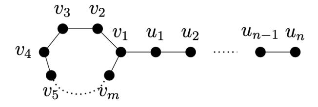
Figure 5. The graph Tm,n.

Next, we show that the recursive formula for the interlace polynomial of the tadpole graph is the same as the interlace polynomial of the path and lollipop graphs. The explicit formula for the interlace polynomial of the tadpole graph has a structure similar to the interlace polynomial of the lollipop graph.

Lemma 3.1. For \[m \ge 3\], \(n \ge 2\), \(q(T_{m,n}) = q(T_{m,n-1}) + xq(T_{m,n-2})\), where \(q(T_{m,0}) = q(C_m)\) and \(q(T_{m,1}) = q(C_m) + xq(P_{m-2})\).

We utilize the following explicit formulas given in [5].

Lemma 3.2. [5] Let P^m be the path of length m (with m+ 1 vertices and m edges) and C^m denote the cycle with m vertices.

1. For m ≥ 2, the interlace polynomial of the path P^m satisfies

\[q(P_m) = \frac{(3+y)(y-1)}{4y} \left(\frac{1+y}{2}\right)^{m+1} + \frac{(3-y)(y+1)}{4y} \left(\frac{1-y}{2}\right)^{m+1}\]

where y = √ 1 + 4x.

2. For \(m \ge 4\), with \(y = \sqrt{1 + 4x}\),

\[q(C_m) = \left(\frac{1-y}{2}\right)^m + \left(\frac{1+y}{2}\right)^m + \frac{y^4 - 10y^2 - 7}{16}\] for \(m\) even,

\[q(C_m) = \left(\frac{1-y}{2}\right)^m + \left(\frac{1+y}{2}\right)^m + \frac{y^2-5}{4}\] for \(m\) odd.

In [2] a general explicit function for \(q(T_{m,n})\) is given for \(m \ge 6, n \ge 5\). Here we provide an alternative form of the explicit function for \(T_{m,n}\) and give results for \(m \ge 3, n \ge 0\).

Theorem 3.1. For \(m \ge 3\) and \(n \ge 0\),

\[q(T_{m,n}) = \frac{q(C_m) + xq(P_{m-2})\gamma}{x(\beta - \gamma)} \left(\frac{1}{\gamma}\right)^{n+1} - \frac{q(C_m) + xq(P_{m-2})\beta}{x(\beta - \gamma)} \left(\frac{1}{\beta}\right)^{n+1}\]

where \(\gamma=\frac{\sqrt{1+4x}-1}{2x}\), \(\beta=\frac{-\sqrt{1+4x}-1}{2x}\) and \(q(C_m)\) and \(q(P_m)\) are the explicit forms given in Lemma 3.2.

Proposition 3.1. For \(m \geq 3\), \(n \geq 1\), \(\deg(q(T_{m,n})) = 1 + \lceil \frac{n}{2} \rceil\), when n is odd and \(\deg(q(T_{m,n})) = 2 + \lceil \frac{n}{2} \rceil\), when n is even.

Proof. Similar to Proposition 2.1.

Proposition 3.2. For \(m \geq 3\), \(n \geq 1\), the independence number \(\alpha(T_{m,n}) = \left\lceil \frac{n-1}{2} \right\rceil + \left\lfloor \frac{m}{2} \right\rfloor\).

Next, we give evaluations of \(T_{m,n}\) at x=1 and -1. Similar to the interlace polynomials of the path and lollipop graphs evaluated at x=1, the interlace polynomial for the tadpole graph evaluated at 1 involves the Fibonacci sequence.

Theorem 3.2. For \(m \ge 3, n \ge 0\),

\[q(T_{m,n})(1) = \begin{cases} (F_{n+1}\sqrt{5} + F_n)F_m + 2F_{n+1}\left(\left(\frac{1-\sqrt{5}}{2}\right)^m - 1\right), & \text{if m is even,} \\ (F_{n+1}\sqrt{5} + F_n)F_m + 2F_{n+1}\left(\frac{1-\sqrt{5}}{2}\right)^m, & \text{if m is odd,} \end{cases}\]

where \(F_n\) is the n-th Fibonacci number with \(F_0 = 0\) and \(F_1 = 1\).

Proof. Fixing \(m \geq 3\), this proof follows by induction on n and Lemma 3.2(2).

Proposition 3.3. For \[m \geq 3, n \geq 0\], let \(C^m = \left(\frac{1 - \sqrt{-3}}{2}\right)^m + \left(\frac{1 + \sqrt{-3}}{2}\right)^m\).

We have that \[C^m = \begin{cases} 2, & \text{if } m \equiv 0 \mod 6, \\ 1, & \text{if } m \equiv 1, 5 \mod 6, \\ -1, & \text{if } m \equiv 2, 4 \mod 6, \\ -2, & \text{if } m \equiv 3 \mod 6, \end{cases}\] and then

Interlace polynomials of lollipop and tadpole graphs | Eubanks-Turner et al.

\[q(T_{m,n})(-1) = \begin{cases} 4, & \text{if } n, m \equiv 0 \mod 6, \\ -1, & \text{if } n \equiv 0 \mod 6; m \equiv 1, 5 \mod 6, \\ 1, & \text{if } n \equiv 0 \mod 6; m \equiv 2, 4 \mod 6, \\ -4, & \text{if } n \equiv 0 \mod 6; m \equiv 3 \mod 6, \end{cases}\] \[\text{[rumus tidak dapat ditampilkan dengan baik — lihat PDF asli]}\] \[-C^m, & \text{if } n \equiv 2 \mod 6,\] \[-q(T_{m,0}), & \text{if } n \equiv 3 \mod 6,\] \[-q(T_{m,1}), & \text{if } n \equiv 4 \mod 6,\] \[-q(T_{m,2}), & \text{if } n \equiv 5 \mod 6\]

\[\begin{array}{l} \textit{Proof. For } m \geq 3, \text{ we have, } C^m = \Big(\frac{1-\sqrt{-3}}{2}\Big)^m + \Big(\frac{1+\sqrt{-3}}{2}\Big)^m = \\ \frac{\Big(1-\sqrt{-3}\Big)^m + \Big(1+\sqrt{-3}\Big)^m}{2^m} = \frac{\Big(2e^{i\frac{\pi}{3}}\Big)^m + \Big(2e^{-i\frac{\pi}{3}}\Big)^m}{2^m} = e^{i\frac{m\pi}{3}} + e^{-i\frac{m\pi}{3}} = 2\cos\frac{m\pi}{3}. \\ \text{Note, that } \cos\frac{m\pi}{3} = \begin{cases} 1, & \text{if } m \equiv 0 \mod 6, \\ \frac{1}{2}, & \text{if } m \equiv 1, 5 \mod 6, \\ -\frac{1}{2}, & \text{if } m \equiv 2, 4 \mod 6, \\ -1, & \text{if } m \equiv 3 \mod 6 \end{cases}. \end{array}\]

Therefore, \(C^m\) is as claimed. Utilizing Lemma 3.2, the remainder of the proof is similar to Proposition 2.2.

Now we consider applications of tadpole graphs in solving a linear algebra problem. For \(n \ge 1\),

let \(B_{mn}\) denote the adjacency matrix of \(T_{mn}\). Then

\[\text{[rumus tidak dapat ditampilkan dengan baik — lihat PDF asli]}\]

\[b_{ij} = \begin{cases} 1, & \text{if } j = i+1 \text{ or } j = i-1, \\ 1, & \text{if } i = 1, j = m \text{ or } i = m, j = 1, \\ 0, & \text{otherwise.} \end{cases}\] \[A_{n \times n} = [a_{ij}], \text{ where } a_{ij} = \begin{cases} 1, & \text{if } j = i+1 \text{ or } j = i-1, \\ 0, & \text{otherwise.} \end{cases}\]

\[A_{n\times n} = [a_{ij}]\], where \(a_{ij} = \begin{cases} 1, & \text{if } j = i+1 \text{ or } j = i-1, \\ 0, & \text{otherwise.} \end{cases}\)

Proposition 3.4. Suppose \(m \ge 3\), \(n \ge 0\), let \(D_{m,n} = B_{m,n} + I_{m+n}\), where \(I_{m+n}\) is the \((m+n) \times I_{m+n}\)(m+n) identity matrix. Then,

\[rank(D_{m,n}) = \begin{cases} m+n-2, & \text{if } n, m \equiv 0, 3 \mod 6, \\ m+n, & \text{if } n \equiv 0, 2, 3, 5 \mod 6; m \equiv 1, 2, 4, 5 \mod 6, \\ m+n-1, & \text{if } n \equiv 1, 4 \mod 6 \text{ and } n \equiv 2, 5 \mod 6; m \equiv 0, 3 \mod 6. \end{cases}\]

Proof. Using Theorem 2.2 and Lemma 3.3, we have the desired result.

Acknowledgement

The work in this manuscript was supported by the RAINS Research Assistantship Program at Loyola Marymount University.

References

• [1] A. Ali, H. Abdullah, and G. Saleh, Hosoya polynomials and Wiener indices of carbon nanotubes using mathematica programming, Journal of Discrete Mathematical Sciences and Cryptography, (2021), 1-12, article in press.
• [2] J. Almeida, Interlace Polynomials of Cycles with One Additional Chord, Theses, Dissertations and Culminating Projects (2018).

• [3] C. Anderson, J. Cutler, A.J. Radcliffe, and L. Traldi, On the interlace polynomials of forests. Discrete Mathematics 310 (1) (2010), 31–36.
• [4] R. Arratia, B. Bollobas, D. Coppersmith, and G. Sorkin, Euler Circuits and DNA sequencing ´ by hybridization, Discrete Applied Mathematics 104 (2000), 63–96.
• [5] R. Arratia, B. Bollobas, and G. Sorkin, The interlace polynomial of a graph, ´ Journal of Combinatorial Theory, 92 (2004), 199–233.
• [6] J. Awan and O. Bernardi, Tutte polynomials for directed graphs, Journal of Combinatorial Theory, Series B, 140 (2020), 192–247.
• [7] P. Balister, B. Bollobas, J. Cutler, and L. Pebody, The interlace polynomial of Graphs at -1, ´ Europ. J. Combinatorics 23 (2002), 761–767.
• [8] A. Bouchet, Graph polynomials derived from Tutte Martin Polynomials, Discrete Mathematics 302 (2005), 32–38.
• [9] F. Chaudhry, M. Husin, F. Afzal, D. Afzal, M. Ehsan, M. Cancan, and M. Farahani, Mpolynomials and degree-based topological indices of tadpole graph, Journal of Discrete Mathematical Sciences and Cryptography 24 (7) (2021), 2059–2072.
• [10] H. Chen and Q. Guo, Tutte polynomials of alternating polycyclic chains, J Math Chem 57 (2019), 2248–2260.
• [11] C. Eubanks-Turner, A. Li, Interlace polynomials of friendship graphs, Electronic Journal of Graph Theory and Applications 6 (2) (2018), 269–281.
• [12] M. Ghorbani, M. Dehmer, S. Cao, L. Feng, J. Tao, F. Emmert-Streib, On the zeros of the partial Hosoya polynomial of graphs, Information Sciences 524 (2020), 199–215.
• [13] A. Li and Q. Wu, Interlace polynomial of ladder graphs, Journal of Combinatorics, Information & System Sciences 35 (2010), 261–273.
• [14] H. Lin, L. Zhang, and J. Xue, Majorization, degree sequence and Aα-spectral characterization of graphs, Discrete Mathematics 343 (12) (2020), 112–132.
• [15] Y. Liu, T. Tan, and M. Yoshinaga, G-Tutte polynomials and abelian lie group arrangements, International Mathematics Research Notices 1 (2) (2021), 150–188.
• [16] S. Nomani and A. Li, Interlace polynomials of n-claw graphs, Journal of Combinatorics and Combinatorial Computing 88 (2014), 111–122.
• [17] A. Seeger and D. Sossa, Extremal problems involving the two largest complementarity eigenvalues of a graph, Graphs and Combinatorics 36 (2020), 1–25.
• [18] L. Traldi, On the interlace polynomials, Journal of Combinatorial Theory, Series B, 103 (2013), 184–208.

[19] Y. Zhang, L. Xiaogang, B. Zhang, and Y. Xuerong, The lollipop graph is determined by its Q-spectrum, Discrete Mathematics 309 (2009), 3364–3369.