A generalization of a Turan's theorem about ma- ´ ximum clique on graphs

Douglas F. G. Santiago, Anderson L. P. Porto, Kaio A. S. Sa´

Institute of Science and Technology (ICT), Federal University of the Jequinhonha and Mucuri Valleys, Diamantina, Brazil

douglas.santiago@ict.ufvjm.edu.br, ander.porto@ict.ufvjm.edu.br, kaioariel1319@gmail.com

One of the most important Turan's theorems establishes an inequality between the maximum clique ´ and the number of edges of a graph. Since 1941, this result has received much attention and many of the different proofs involve induction and a probability distribution. In this paper we detail finite procedures that gives a proof for the Turan's Theorem. Among other things, we give a ´ generalization of this result. Also we apply this results to a Nikiforov's inequality between the spectral radius and the maximum clique of a graph.

Keywords: maximum clique, spectral radius, Turan's theorem, probability distribution ´

Mathematics Subject Classification : 05C35, 05C50, 05C69

DOI: 10.5614/ejgta.2022.10.2.10

1. Introduction

Many works in graph theory deals with upper bounds for the number of edges in a graph. Some examples are [5], [9] and [6]. In this scope, the famous Turan's Theorem is one of the most ´ important results in graph theory about cliques and the number of edges in a graph and is stated as follows

Theorem 1.1. (Turan) ´ Consider p ≥ 2 an integer. Let G be a simple graph with n vertices and m

Received: 19 March 2021, Revised: 6 July 2022, Accepted: 17 July 2022.

edges not containing a p-clique, then

\[m \le \left(1 - \frac{1}{p-1}\right) \frac{n^2}{2}.\tag{1}\]

This result gives the maximum number of edges that a simple graph of n vertices can have if it doesn't contain a clique of a certain size [10]. Also this result provides what is known as extremal problems in graph theory [3]. We recommend [1] for some proofs.

In [1] there are four proofs of Theorem 1.1. The third proof present a sketch of procedures to prove the theorem and was based on ideas in [2, 7] and [11]. In [7] the proofs are based on finite induction and in [7, 11] there are generalizations of Turán's theorem. Theorem 1.1 was utilized by Nikiforov in [8] to relate the spectral radius and the maximum clique of a graph.

Theorem 1.2. (Nikiforov) Let G be a simple graph with n vertices having the spectral radius \(\lambda\) and cl(G) the cardinality of a maximum clique. Then

\[\lambda \le \left(1 - \frac{1}{cl(G)}\right)n. \tag{2}\]

In this paper we detail the procedures described in [1] to obtain better inequalities involving not only the clique number but also the amount of some cliques in the graph. As consequence we apply these inequalities to improve Nikiforov's Theorem 1.2.

The rest of the paper is organized as follows: In section 3 we present the detailed procedures developed. These are described in the proofs of Theorems 3.1 and 3.2. In section 4 we develop our improved inequalities.

2. Notations

In this paper we will denote by \(G=(V(G),E(G),\psi_G)\) a finite unoriented graph with V(G)=V the set of vertices, E(G)=E the set of edges and \(\psi_G\) the incidence function. If there is no confusion, we will simply make mention to the graph G. The vertices will be denoted by v (or \(v_i\)) and the edges by \(e=v_iv_j\). N(v) will be the set containing all neighboring vertices of the vertex v. If v is included in the set, we have a star \(\overline{N}(v)=N(v)\cup\{v\}\). A particular k-clique in G sometimes will be denoted \(Cl_k(G)\). The cardinality of a maximum clique will by cl(G). Let A, B be non-empty subsets of V. A and B are disconnected if there is no \(a\in A\) and \(b\in B\) such that \(ab\in E\). We will denote by |X| the cardinality of set X, \(\langle a,b\rangle\) the canonical scalar product of a and \(b\in B\) and \(b\in B\) and \(b\in B\) and \(b\in B\) and \(b\in B\) and \(b\in B\) and \(b\in B\) and \(b\in B\) and \(b\in B\) and \(b\in B\) and \(b\in B\) and \(b\in B\) and \(b\in B\) and \(b\in B\) and \(b\in B\) and \(b\in B\) and \(b\in B\) and \(b\in B\) and \(b\in B\) and \(b\in B\) and \(b\in B\) and \(b\in B\) and \(b\in B\) and \(b\in B\) and \(b\in B\) and \(b\in B\) and \(b\in B\) and \(b\in B\) and \(b\in B\) and \(b\in B\) and \(b\in B\) and \(b\in B\) and \(b\in B\) and \(b\in B\) and \(b\in B\) and \(b\in B\) and \(b\in B\) and \(b\in B\) and \(b\in B\) and \(b\in B\) and \(b\in B\) and \(b\in B\) and \(b\in B\) and \(b\in B\) and \(b\in B\) and \(b\in B\) and \(b\in B\) and \(b\in B\) and \(b\in B\) and \(b\in B\) and \(b\in B\) and \(b\in B\) and \(b\in B\) and \(b\in B\) and \(b\in B\) and \(b\in B\) and \(b\in B\) and \(b\in B\) and \(b\in B\) and \(b\in B\) and \(b\in B\) and \(b\in B\) and \(b\in B\) and \(b\in B\) and \(b\in B\) and \(b\in B\) and \(b\in B\) and \(b\in B\) and \(b\in B\) and \(b\in B\) and \(b\in B\) and \(b\in B\) and \(b\in B\) and \(b\in B\) and \(b\in B\) and \(b\in B\) and \(b\in B\) and \(b\in B\) and \(b\in B\) and \(b\in B\) and \(b\in B\) and \(b\in B\) and \(b\in B\) and \(b\in B\) and \(b\in B\) and \(b\in B\) and \(b\in B\) and \(b\in B\) and \(b\in B\) and \(b\in B\) and \(b\in B\) and \(b\in B\) and \(b\in B\) and \(b\in B\) and \(b\in B\) and \(b\in B\) and \(b\in B\) and \(b\in B\) and \(b\in B\) and \(b\in B\) and \(b\in B\) and \(b\in B\) and \(b\in B\) and \(b\in B\) and \(b\in B\) and \(b\in B\) and \(b\in B\) and \(b\in B\) and \(b\in B\) and \(b\in B\) and \(b\in B\) and \(b\in B\) and \(b\in\)

We define the set

\[D = \left\{ w = (w_1, \dots, w_n) \in \mathbb{R}^n \,\middle|\, w_i \ge 0 \text{ e } \sum_{i=1}^n w_i = 1 \right\}.\] (3)

Let G be a finite graph. All proofs of the following results were based on maximizing the function \(f_G: D \to \mathbb{R}\) such that

\[f_G(w) = \sum_{v_i v_j \in E(G)} w_i w_j. \tag{4}\]

Each wⁱ represents the weight of the vertex vⁱ and w = (w1, . . . , wn) is the (discrete) probability distribution over V (G). If ψG(ek) = viv^j we say that wiw^j is the weight of the edge ek. In this way, fG(w) gives the sum of all the weights of the edges of G. For the rest of the article, we will only consider graphs with at least one edge. The weight of a non-empty set A ⊂ V (G) is the sum of all weights of the vertices v ∈ A. Furthermore, denote by s^r the sum of the weights of N(vr) for r ∈ {1, . . . , n}.

3. Procedures

In this section let w = (w1, . . . , wn) be a probability distribution over V (G). We present two Theorems indicating finite procedures on the weights of a distribution w that forms the base for the proof of our main results.

Lemma 3.1. Let G be a non-complete graph with V (G) = {v1, v2, . . . , vn}. Take w and w ′ = (w ′ 1 , . . . , w′ n ) two probabilities distributions over V (G) and vⁱ , v^j two non-adjacent vertices such that sⁱ ≥ s^j in w distribution. Let w ′ ^j = 0, w ′ ⁱ = wⁱ + w^j and w ′ ^k = w^k for k ̸= i, j. Then fG(w ′ ) ≥ fG(w).

Proof. Note that fG(w ′ ) is the same as fG(w) plus w^j multiplied by all weights related to the adjacencies of vⁱ (since w ′ ⁱ = wⁱ + w^j ), and plus −w^j multiplied by all weights related to the adjacencies of v^j (since w ′ ^j = 0), then:

\[f_G(w') = f_G(w) + w_j s_i - w_j s_j = f_G(w) + w_j (s_i - s_j).\] (5)

As sⁱ ≥ s^j then wi(sⁱ − s^j ) ≥ 0 and we conclude that

\[f_G(w') \ge f_G(w). \tag{6}\]

Theorem 3.1. Let G be a simple graph with n vertices. For all probability distribution w on V (G), there is a k-clique, say Clk(G), and a probability distribution w = (w1, . . . ,wn) with fG(w) ≥ fG(w) and wⁱ = 0 for all vⁱ ∈/ Clk(G).

Proof. The proof is based on a finite procedure. If G is complete, we will consider that there is nothing to do and the theorem is proved. Suppose then that G is a non-complete graph. Take sⁱ the weight of N(vi) for all vⁱ ∈ V (G). Reorder the vertices of G such that s¹ ≥ s² ≥ · · · ≥ sn. Since G is not complete, let vⁱ¹ be the first vertex in the chosen order that does not have all the vertices of G connected to it. For each vertex disconnected with vⁱ¹ create a new distribution w ′ as explained in Lemma 3.1. Note that in all steps the relation sⁱ¹ ≥ s^j is still valid for vertices v^j disconnected to vⁱ¹ . At the end all the vertex disconnected to vⁱ¹ has zero weight. If all vertices of N(vⁱ¹ ) are connected to each other, then N(vⁱ¹ ) is a |N(vⁱ¹ )|-clique satisfying the thesis of this theorem.

Otherwise, among all the vertices connected to \(v_{i_1}\) find one, say \(v_{i_2}\), such that it is not connected to all vertices of \(N(v_{i_1})\) whose value of \(s_{i_2}\) is maximum between those vertices in \(N(v_{i_1})\). Repeat the procedure now with vertex \(v_{i_2}\). Make this until we have a probability distribution \(\overline{w}\) such that the only weights \(\overline{w}_i \neq 0\) are concentrated in a k-clique, \(Cl_k(G)\). By Lemma 3.1 we have \(f_G(\overline{w}) \geq f_G(w)\).

If \(w=(w_1,\ldots,w_n)\) is a probability distribution on V(G), we will say that w is also a probability distribution on a k-clique \(Cl_k(G)=\{v_{i_1},\ldots,v_{i_k}\}\) if \(w_j=0\) for all vertices \(v_j\) not in \(Cl_k(G)\). Remember that a homogeneous probability distribution has all weights equal. The next lemma shows that for all probability distributions w on a k-clique \(Cl_k(G)\), the homogeneous probability distribution \(\overline{w}\) on the k-clique \(Cl_k(G)\) satisfies \(f_G(\overline{w}) \geq f_G(w)\).

Lemma 3.2. Let G be a simple graph with n vertices and consider w a probability distribution over a k-clique \(Cl_k(G)\). Let \(v_i, v_j\) be two vertices of \(Cl_k(G)\) satisfying \(w_i \geq w_j\), moreover consider \(\varepsilon \in \mathbb{R}\) such that \(0 \leq \varepsilon \leq w_i - w_j\). The probability distribution w' on \(Cl_k(G)\) such that \(w'_i = w_i - \varepsilon\), \(w'_j = w_j + \varepsilon\) and \(w'_k = w_k\) for all \(i \neq k \neq j\) satisfies \(f_G(w') \geq f_G(w)\).

Proof. It is easy to see that

\[f_G(w') = f_G(w) + \varepsilon(w_i - w_i - \varepsilon). \tag{7}\]

and then we conclude \(f_G(w') \ge f_G(w)\).

Theorem 3.2. Let G be a simple graph with n vertices. For any probability distribution w on a clique, say \(Cl_k(G)\), the homogeneous probability distribution \(\overline{w}\) satisfies \(f_G(\overline{w}) \geq f_G(w)\).

Proof. Consider an enumeration of the vertices of \(Cl_k(G)=\{v_1,\ldots,v_k\}\) satisfying \(w_1\leq w_2\leq\ldots\leq w_k\) and define the set \(A^0=\{v_1,\ldots,v_r\}\subset Cl_k(G)\) such that \(w_j=w_1\) for \(j\in\{1,\ldots,r\}\). If \(A^0=Cl_k(G)\) there is nothing to do, else, consider the vertex \(v_{r+1}\) with weight \(w_{r+1}\). Take \(\varepsilon=\frac{w_{r+1}-w_1}{r+1}>0\). Consider a probability distribution \(w^1\) such that \(w_{r+1}^1=w_{r+1}-\varepsilon,w_r^1=w_r+\varepsilon\) and \(w_k^1=w_k\) for all \(k\neq r\neq r+1\). By Lemma 3.2 \(f_G(w^1)\geq f_G(w)\). Consider a probability distribution \(w^2\) such that \(w_{r+1}^2=w_{r+1}^1-\varepsilon=w_{r+1}-2\varepsilon,w_{r-1}^2=w_{r-1}+\varepsilon,w_r^2=w_r^1\) and \(w_k^2=w_1\) for \(k\in\{1,\ldots,r-2\}\). Again by Lemma 3.2, we have \(f_G(w^2)\geq f_G(w)\). At the end of this process we have a set \(A^1=\{v_1,\ldots,v_r,v_{r+1}\}\supset A^0\) where all vertices have weights equal to \(w_1+\varepsilon\). If \(A^1=Cl_k(G)\) there is nothing to do, otherwise repeat the process until we have a homogeneous probability distribution \(\overline{w}\) on the clique \(Cl_k(G)\). According Lemma 3.2, we have \(f_G(\overline{w})\geq f_G(w)\).

4. Results

Equations (1) and (2) can estimate, respectively, the number of edges and the spectral radius of a simple graph based on the maximum clique. We will show how the number of edges can also depend on the number of cliques of the graph (maximum or not). Consequently, based on the proof of Theorem 1.2, we improve the results as long as we previously know some disconnected cliques in the graph.

4.1. Generalization of Turán's Theorem

Theorem 4.1. Let G be a simple graph with n vertices. Assume the following conditions:

• i) G contains a collection \(CL = \{A_i | i \in \{1, ..., r\}\}\) of disconnected cliques \(A_i\) with cardinality \(k_i\);
• ii) \(\overline{v}\) is a vertex of maximum degree in G;
• iii) Star \(\overline{N}(\overline{v})\) is disconnected from any clique \(A_i\) in \(\mathcal{CL}\).

Then

\[|E| \le \left[ (1 - \gamma)^2 \left( 1 - \frac{1}{k} \right) + \sum_{i=1}^r \left( \frac{k_i}{n} \right)^2 \left( 1 - \frac{1}{k_i} \right) \right] \frac{n^2}{2},\] (8)

where k is the cardinality of a k-clique \(Cl_k(G)\) from G containing \(\overline{v}\) and \(\gamma = \frac{1}{n} \sum_{i=1}^r k_i\);

Proof. Take a homogeneous probability distribution w on V(G). We have \(f_G(w) = |E| \frac{1}{n^2}\). Clearly the vertices v such that the weight of N(v) are maximum are those with maximum degree. Let A be the set of all vertices of G that are not vertices of any of the cliques in the \(\mathcal{CL}\) collection. Apply then the procedure described in Theorem 3.1 in vertex \(\overline{v}\) with the vertices of set A until there is a probability distribution over A that is null in \(A \setminus Cl_k(G)\), where \(Cl_k(G)\) is a k-clique from G containing \(\overline{v}\). Apply then the procedure described in Theorem 3.2 on \(Cl_k(G)\) until all the vertices weights in \(Cl_k(G)\) be equal. After these procedures, all vertex weights in \(\mathcal{CL}\) are equal to \(\frac{1}{n}\) and all vertex weights in \(Cl_k(G)\) are equal to \(\frac{1-\gamma}{k}\).

By Lemmas 3.1 and 3.2 we have then a new distribution w' on G, such that \(|E|\frac{1}{n^2}=f_G(w) \leq f_G(w')=B_1+B_2\), where \(B_1=\frac{1}{2}\cdot(1-\gamma)^2\left(1-\frac{1}{k}\right)\) represents the contribution from \(Cl_k(G)\) and \(B_2=\frac{1}{2}\cdot\sum_{i=1}^r\left[\left(\frac{k_i}{n}\right)^2\cdot\left(1-\frac{1}{k_i}\right)\right]\) represents the contribution from \(\mathcal{CL}\). Solving the inequality the result follows.

In Equation (8), note that \(\sum_{i=1}^{r} \left(\frac{k_i}{n}\right)^2 \left(1 - \frac{1}{k_i}\right) \frac{n^2}{2} = \sum_{i=1}^{r} \frac{k_i(k_i-1)}{2}\), i.e, the amount of the edges considering all the cliques in \(\mathcal{CL}\).

If there are no cliques on \(\mathcal{CL}\) the previous theorem is reduced to Theorem 1.1.

We can obtain a shorter inequality from Theorem 4.1, taking account that \(\left(1 - \frac{1}{k}\right) \leq \left(1 - \frac{1}{cl(G)}\right)\) for all clique \(Cl_k(G)\). Then we have

Corollary 4.1. With the same hypotheses as the previous theorem, we have

\[|E| \le \varsigma \left(1 - \frac{1}{cl(G)}\right) \frac{n^2}{2},\tag{9}\]

where \(\varsigma = \left[ (1 - \gamma)^2 + \sum_{i=1}^r \left( \frac{k_i}{n} \right)^2 \right].\)

It is clear that \(\gamma\) and \(\frac{k_i}{n} \in [0,1], \forall i=1,\ldots,r\), moreover \(\gamma + \sum_{i=1}^r \left(\frac{k_i}{n}\right) = 1\), then \(\varsigma < 1\) and inequality (9) is better than inequality (1).

4.2. Generalization of Nikiforov's Theorem

Theorem 4.2. With the same hypotheses as Theorem 4.1 we have that the spectral radius \(\lambda\) satisfies

\[\lambda \le \sqrt{\varsigma} \left( 1 - \frac{1}{cl(G)} \right) n,\tag{10}\]

where \(\varsigma = \left[ \left( 1 - \gamma \right)^2 + \sum_{i=1}^r \left( \frac{k_i}{n} \right)^2 \right].\)

Proof. If |E(G)| = 0 then \(\lambda = 0\) and the result is obvious. Suppose from now on that \(|E(G)| \ge 1\).

Fix an enumeration of the vertices of G. Let A be its respective adjacency matrix and \(y = \begin{bmatrix} y_1 \\ \vdots \\ y_n \end{bmatrix}\)

a unit eigenvector related to \(\lambda\) that is, ||y||=1. We know that:

\[\lambda = \langle y, Ay \rangle \,. \tag{11}\]

Take \(z = \begin{bmatrix} z_1 \\ \vdots \\ z_n \end{bmatrix} = Ay\). Each entry \(z_i\) is exactly the sum of the y entries associated with the

vertices adjacent to \(v_i\)

Let l = |E(G)| and consider an enumeration \(e_1 < \ldots < e_l\) of the l edges of G. For each \(k = 1, \ldots, l\), let \(e_k = v_i^k v_j^k\) the k-th edge of G associated with the number \(y_i^k \cdot y_j^k\) such that \(y_i^k, y_j^k \in \{y_1, \ldots, y_n\}\) which are the coordinates of the y vector. Then in the inner product (11) we have:

\[\lambda = 2 \sum_{v_i^k v_i^k \in E(G)} y_i^k y_j^k = 2 \sum_{v_i v_j \in E(G)} y_i y_j.\] (12)

The number 2 comes from symmetry of A. We can then rewrite Equation (12) as the inner product

between the vector \(r = \begin{bmatrix} 2 \\ \vdots \\ 2 \end{bmatrix} \in \mathbb{R}^l\) and the vector \(s = \begin{bmatrix} z_1 \\ \vdots \\ z_l \end{bmatrix} \in \mathbb{R}^l\) whose entries are the values

\(z_t = y_i^t y_j^t\):

\[\lambda = \langle r, s \rangle \,. \tag{13}\]

We also have:

\[||r|| = \sqrt{2^2 + \dots + 2^2} = \sqrt{4|E|},\] (14)

as long as:

\[||s|| = \sqrt{\sum_{v_i v_j \in E(G)} y_i^2 y_j^2}.\] (15)

By Cauchy-Schwartz inequality, we have:

\[\langle r, s \rangle^2 \le ||r||^2 \cdot ||s||^2.\] (16)

Replacing Equation (13), (14) and (15) in Equation (16), we get:

\[\lambda^2 \le 4|E| \cdot \sum_{v_i v_j \in E(G)} y_i^2 y_j^2. \tag{17}\]

Because y is unitary, w = (y 2 1 , . . . , y² n ) is a probability distribution on V (G).

Through combinatorial analysis it is easy to see that the number of edges E^k in the complete graph induced by a k-clique is equal to:

\[|E_k| = \frac{k(k-1)}{2}. (18)\]

Then a k-clique with homogeneous probability distribution w ′ satisfies

\[f_G(w') = |E_k| \frac{1}{k^2}. (19)\]

Replacing Equation (18) in Equation (19), we get:

\[f_G(w') = \left(1 - \frac{1}{k}\right) \frac{1}{2}.\] (20)

According procedures explained in Theorem3.1 and Theorem 3.2, for any probability distribution w, there is a k-clique such that:

\[f_G(w) \le \left(1 - \frac{1}{k}\right) \frac{1}{2}.\tag{21}\]

We have k ≤ cl(G), so we conclude that:

\[\sum_{v_i v_j \in E(G)} y_i^2 y_j^2 \le \left(1 - \frac{1}{cl(G)}\right) \frac{1}{2},\tag{22}\]

Replacing Equation (22) in Equation (17), we get:

\[\lambda^2 \le 2|E| \left( 1 - \frac{1}{cl(G)} \right). \tag{23}\]

As discussed in Corollary 4.1: |E| ≤ ς 1 − 1 cl(G) n 2 2 and the result follows.

If there are no clique on CL the previous theorem is reduced to Theorem 1.2. The next corollary is straightforward.

Corollary 4.2. With the same hypotheses as Theorem 4.1, we have that the cardinality of the maximum clique cl(G) satisfies

\[cl(G) \ge \frac{n}{n - \frac{\lambda}{\sqrt{\varsigma}}},\] (24)

where \[\varsigma = \left[ (1 - \gamma)^2 + \sum_{i=1}^r \left( \frac{k_i}{n} \right)^2 \right].\]

Here is an example. Let G be the graph with 12 vertices and 14 edges of Figure 1. Its spectral radius \(\lambda=2.6729197\), the cardinality of the maximum clique is cl(G)=3 and the maximum degree in the graph is equal to 4.

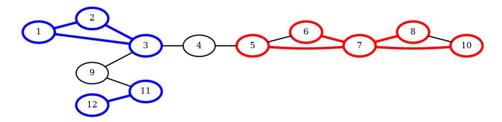
Figure 1. Graph G.

In blue, we have a 2-clique \(Cl_2(G)\), a 3-clique \(Cl_3(G)\) and in red a star \(\overline{N}(\overline{v_7})\) all disconnected. With this sets we have \(\varsigma=\frac{31}{72}\) and according Equation (9) in Corollary 4.1, \(|E|\leq 20.6666667\) (Equation (1) gives \(|E|\leq 48\)). According Equation (10) in Theorem 4.2, \(\lambda\leq 5.249339\) (Equation (2) gives \(\lambda\leq 8\)).

It follows another example. Let H be the graph with 30 vertices and 33 edges of Figure 2. Its spectral radius \(\lambda=2.9883861\), the cardinality of the maximum clique is cl(H)=2 and the maximum degree in the graph is equal to 6.

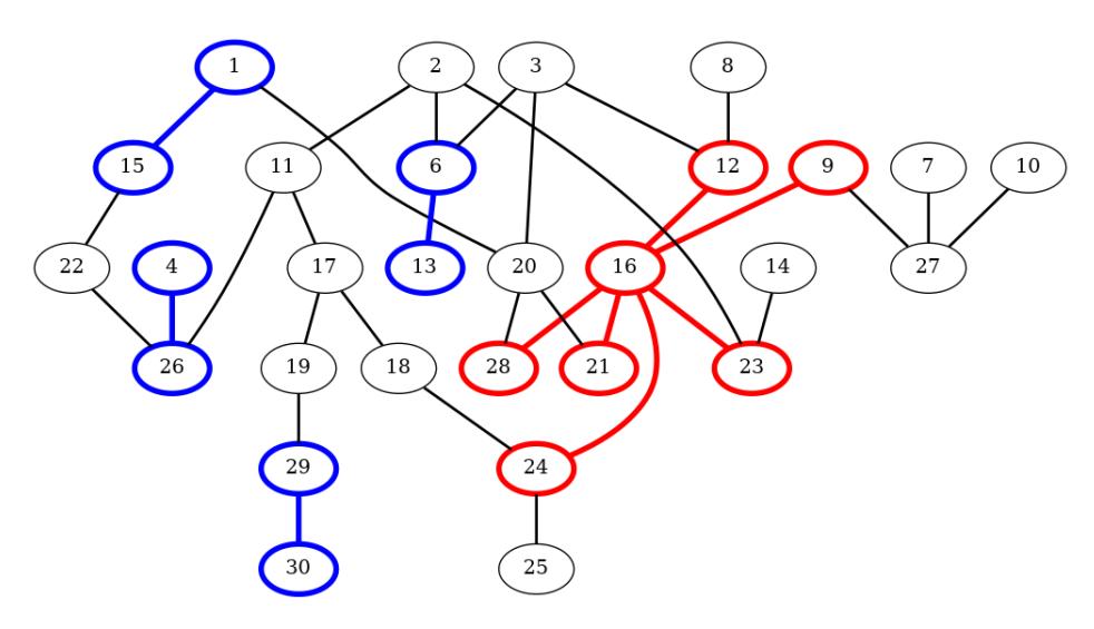
Figure 2. Graph H.

In blue, we have four 2-cliques and in red a star N(v16) all disconnected. With this sets we have ς = 5 9 and according Equation (9) in Corollary 4.1, |E| ≤ 125 (Equation (1) gives |E| ≤ 225 ). According Equation (10) in Theorem 4.2, λ ≤ 11.180340 (Equation (2) gives λ ≤ 15).

References

• [1] M. Aigner and G.M. Ziegler, Turan's Graph Theorem, In: ´ Proofs from the Book. Berlin, Heidelberg: Springer, (1998), 169-172.
• [2] N. Alon and J. Spencer, The Probalilistic Method, 2 edn. Tel Aviv and New York, Wiley Interscience, (2000).
• [3] B. Bollobas, ´ Extremal Graph Theory, Reprint of the 1978 original. Mineola, NY: Dover Publications, (2004).
• [4] J. Bondy, and U. Murty, Graph Theory, 1 edn. Springer Publishing Company, (2008).
• [5] L. Eroh, H. Escuadro, R. Gera, and S. Prahlow, S, A graph theoretical analysis of the number of edges in k-dense graphs, Electron. J. Graph Theory Appl. 4 (1) (2016), 26–41.
• [6] M. Hailat, An upper bound of edges of graphs containing no vertex-disjoint odd cycles, J. Math. Comput. Sci. 8 (6) (2018), 644–653.
• [7] T.S. Motzkin and E.G. Straus, Maxima for graphs and a new proof of a theorem of Turan. ´ Can. J. Math 17 (1965), 533–540. https://doi.org/10.4153/CJM-1965-053-6.
• [8] V. Nikiforov, Some inequalities for the largest eigenvalue of a graph, Combin. Probab. Comput. 11 (2002), 179–189. https://doi.org/10.1017/S0963548301004928.
• [9] V.S. Samoilov, An upper bound on the number of edges of a graph whose k-th power has a connected complement, Journal of Mathematical Sciences 232 (1) (2018) .
• [10] P. Turan, On an extremal problem in graph theory (in Hungarian). ´ Mat. Fiz. Lapok, 48 (1941), 436–452.
• [11] P. Turan, On the theory of graphs, ´ Colloq. Math 3 (1954), 19–30. https://doi.org/10.4064/cm-3-1-19-30.