Richard M. Lowa , Ardak Kapbasova , Arman Kapbasovb , Sergey Beregc
richard.low@sjsu.edu, ardak.kapbasov@yahoo.com, akapbasov@fb.com, sbereg@gmail.com
For various connected simple graphs G, we extend the table of diagonal graph Ramsey numbers R(G, G) in 'An Atlas of Graphs.' This is accomplished by first converting the calculation of R(G, G) into a satisfiability problem in propositional logic. Mathematical arguments and scientific computing are then used to calculate R(G, G).
Keywords: Graph Ramsey theory, diagonal Ramsey numbers
2020 Mathematics Subject Classification: 05C55
DOI: 10.5614/ejgta.2022.10.2.17
1. Introduction
In 1929, Frank Ramsey [20] established an innocuous-looking theorem in his groundbreaking paper on formal logic. Although it was not apparent at the time, Ramsey's theorem would eventually form the cornerstone of Ramsey theory, a vibrant and rich area of extremal combinatorics.
The following general question [12] is investigated in Ramsey theory.
• If a particular mathematical structure (e.g., algebraic, combinatorial, or geometric) is arbitrarily partitioned into finite many classes, what kinds of substructures must always remain intact in at least one of the classes?
Received: 29 January 2022, Revised: 2 October 2022, Accepted: 9 October 2022.
aDepartment of Mathematics and Statistics, San Jose State University, San Jose, CA 95192, USA bFacebook, 1 Hacker Way, Menlo Park, CA 94025, USA
cDepartment of Computer Science, University of Texas at Dallas, Richardson, TX 75083, USA
Over many decades, Ramsey-type questions in mathematical structures such as the integers [16], graphs, and Euclidean space have been investigated. As of this writing, a keyword search for "Ramsey" yields 2926 entries in the MathSciNet database. The interested reader is directed to [12, 13] for a comprehensive overview of Ramsey theory. For a gentle introduction to Ramsey theory, [22] is recommended.
Applications of Ramsey theory can be found in number theory, algebra, geometry, topology, set theory, logic, ergodic theory, information theory and computer science. The reader is directed to Rosta's [23] survey for a detailed exposition of some of these applications.
The reader should note that the seeds of Ramsey theory were planted even before Ramsey introduced his theorem. Soifer's [25] beautifully written book is filled with deep mathematics and also provides a rich historical context of Ramsey theory.
2. Preliminaries
The focus of this paper is on calculating new diagonal Ramsey numbers in graph Ramsey theory.
First, we recall some standard definitions and notation from graph theory. All graphs are finite, simple and connected. Any notation and terminology which are not explicitly defined in this paper can be found in [12, 27]. For a graph G with vertex set V (G) and edge set E(G), the order and size of G are defined to be |V (G)| and |E(G)|, respectively. The complete graph Kn is the simple graph on n vertices, where every pair of vertices are adjacent.
In graph Ramsey theory, the following definitions and notation are used.
Definition 1. Let k ≥ 2. A r-coloring of G is a coloring of E(G), using a maximum of r colors.
Notation 1. Let G and H be simple connected graphs. If every 2-coloring of Kn yields a monochromatic subgraph G or a monochromatic subgraph H in Kn, then this is denoted by Kn → (G, H). If that is not the case, then the notation Kn ↛ (G, H) is used.
Definition 2. The Ramsey number R(G, H) is defined to be the minimum n, where Kn → (G, H).
Using graph-theoretic language, the finite version of Ramsey's theorem can be stated in the following way.
Theorem A. (Ramsey [20]). Let s, t ≥ 2. Then, there exists a minimal positive integer n such that every edge coloring of Kn (using two colors) contains a monochromatic Ks or a monochromatic Kt .
Considerable work has been done in graph Ramsey theory. In addition to the calculation of Ramsey numbers in the classical theory, many different concepts have been introduced over time. They include Ramsey functions on graphs, many kinds of mixed Ramsey numbers, size Ramsey numbers, connected Ramsey numbers, anti-Ramsey numbers and Gallai-Ramsey numbers. These topics (and many others) can be found within the extensive mathematical literature. For an overview of classical graph Ramsey theory, the general surveys of Burr [1, 2], Radziszowski [19], Read and Wilson [21], and Sudakov [26] are invaluable. New directions and additional open questions in graph Ramsey theory are addressed in [4, 29, 30].
3. Calculating R(G, H) using propositional logic
For a mathematical introduction to logic, the reader is directed to [11]. We begin by recalling two concepts from propositional logic. A conjunctive normal form (CNF) is a Boolean expression consisting of a conjunction of disjunctions of propositional statements or their negations. An example of a CNF would be
\[(A \vee \neg B \vee \neg C) \wedge (\neg A \vee \neg B) \wedge (\neg A \vee \neg B \vee C),\]
where A, B and C represent propositional statements and ∨, ∧ and ¬ represent "OR," "AND" and "NOT," respectively. A Boolean expression is satisfiable if there is an assignment of "true" and "false" values to its propositional statements which makes the expression "true" (when evaluated using the standard truth table rules).
Cowen [9] used Mathematica's Boolean computational abilities to investigate some questions from graph Ramsey theory. In particular, he converted the problem of calculating R(Ks, Kt) into a satisfiabilty problem. Here is an overview of his approach.
Cowen's approach: Let s, t, and n be integers with 2 < s, t < n, and Kn be the complete graph with vertices numbered 1, 2, . . . , n. For each pair of integers (i, j), where i, j ∈ V (Kn) with 1 ≤ i < j ≤ n, construct a CNF f (called "RamseyTest"), using variables ri,j and bi,j which denote the edge ei,j ∈ E(Kn) being colored red or blue, respectively. The CNF f consists of two sets of clauses:
- (Coloring clauses). For each pair of integers (i, j) with 1 ≤ i < j ≤ n, the clauses ri,j ∨ bi,j and ¬ri,j ∨ ¬bi,j provide a valid 2-coloring of Kn.
- (Non-monochromatic subgraph clauses). These clauses make sure that a 2-coloring of Kn does not contain a monochromatic Ks or Kt .
If f is not satisfied, then Kn → (Ks, Kt). In this case, R(Ks, Kt) ≤ n. If f is satisfied, then Kn ↛ (Ks, Kt). In this case, n + 1 ≤ R(Ks, Kt).
Example 1. Suppose we wish to determine if R(K3, K3) ≤ 4. Using the Wolfram Language in Mathematica [28], the (combined) coloring and non-monochromatic subgraph clauses are, respectively:
Here, | | denotes "OR," && denotes "AND," and ! denotes "NOT." The two sets of clauses are connected by && in f. ♢
Cowen then improved the efficiency of his "RamseyTest" CNF by noting the following fact: In any 2-coloring of Kn, at least half of the edges from a particular vertex are of the same color (say, red). Thus, he created a new CNF f0 called "QuickerRamseyTest" which utilized this observation. This modest optimization decreased the runtime of "RamseyTest" significantly. For example, f0 determined that R(K4, K4) = 18 in approximately 4.5 seconds. In stark contrast to this, "RamseyTest" could not calculate R(K4, K4) in a reasonable amount of time and had to be manually
Out[5]= (red[{1, 2}] || blue[{1, 2}]) &&
       (! red[{1, 2}] || ! blue[{1, 2}]) &&
       (red[{1, 3}] || blue[{1, 3}]) &&
       (! red[{1, 3}] || ! blue[{1, 3}]) &&
       (red[{1, 4}] || blue[{1, 4}]) &&
       (! red[{1, 4}] || ! blue[{1, 4}]) &&
       (red[{2, 3}] || blue[{2, 3}]) &&
       (! red[{2, 3}] || ! blue[{2, 3}]) &&
       (red[{2, 4}] || blue[{2, 4}]) &&
       (! red[{2, 4}] || ! blue[{2, 4}]) &&
       (red[{3, 4}] || blue[{3, 4}]) && (! red[{3, 4}] || ! blue[{3, 4}])
Out[6]= (! red[{1, 2}] || ! red[{1, 3}] || ! red[{2, 3}]) &&
       (! red[{1, 2}] || ! red[{1, 4}] || ! red[{2, 4}]) &&
       (! red[{1, 3}] || ! red[{1, 4}] || ! red[{3, 4}]) &&
       (! red[{2, 3}] || ! red[{2, 4}] || ! red[{3, 4}]) &&
       (! blue[{1, 2}] || ! blue[{1, 3}] || ! blue[{2, 3}]) &&
       (! blue[{1, 2}] || ! blue[{1, 4}] || ! blue[{2, 4}]) &&
       (! blue[{1, 3}] || ! blue[{1, 4}] || ! blue[{3, 4}]) &&
       (! blue[{2, 3}] || ! blue[{2, 4}] || ! blue[{3, 4}])
terminated.
In [9], Cowen explored R(G1, G2, G3), where Gi were complete graphs. We ask the natural question "Is it feasible to adapt Cowen's approach to compute new diagonal graph Ramsey numbers R(G, G), where G is any simple connected graph?"
Our hybrid approach: To further improve the efficiency of Cowen's "QuickerRamseyTest," we make additional use of Kn's symmetry when creating the 2-colorings of it. Let G be a simple connected graph. We want to decide if Kn → (G, G) or not. Let k ≤ n. Now, fix k and consider G(k), the set of nonisomorphic simple graphs of order k. For a graph H ∈ G(k), color the edges of H in red and the edges of H (the complement of H) in blue. Then, embed H and H (with vertices v1, v2, . . . , vk) in Kn (with vertices v1, v2, . . . , vn).
As in Cowen's approach, create a CNF f(H) using coloring clauses and non-monochromatic subgraph clauses. If f(H) is not satisfied for all H ∈ G(k), then Kn → (G, G). In this case, R(G, G) ≤ n. If f(H) is satisfied for some H ∈ G(k), then Kn ↛ (G, G). In this case, n + 1 ≤ R(G, G).
Example 2. Let G be a simple connected graph where |V (G)| = 7, say. Suppose that we want to determine if R(G, G) ≤ 9. There is a one-to-one correspondence between the set G(8) of nonisomorphic simple graphs of order eight and the set C(K8) of nonequivalent 2-colorings of K8.
Consider a simple graph H ∈ G(8) with k = 8 vertices (see Figure 1), with H being the complement of H. Associated with H is a partial 2-coloring CH of K9, where the edges of H and H are red and blue, respectively. A CNF f(H) is created using clauses for the 2-colorings of K9 containing CH, along with clauses for the non-monochromatic subgraphs (∼= G) of K9. Then, f(H) is tested for satisfiability. Since there are 12346 nonisomorphic simple graphs with eight vertices, 12346 CNFs f(Hi) in total need to be constructed and tested for satisfiability. If all of the f(Hi) are unsatisfied, then R(G, G) ≤ 9. If at least one of the f(Hi) is satisfied, then R(G, G) > 9. ♢
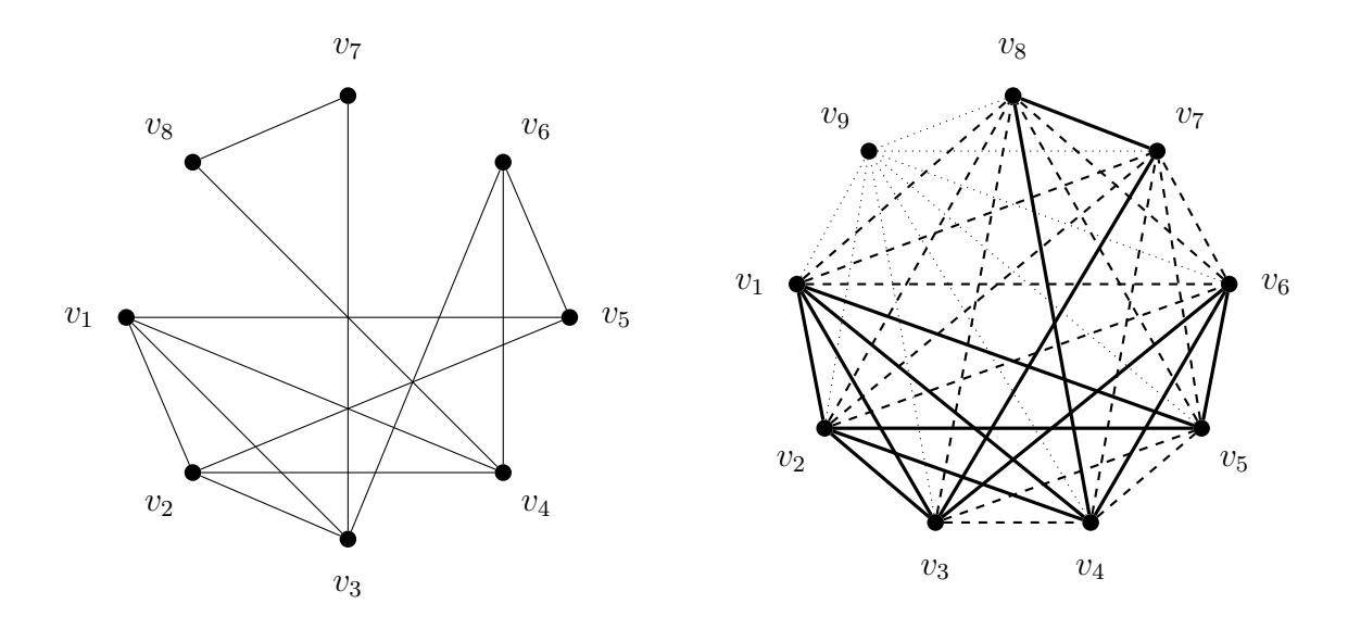
Figure 1: The graph on the left is an H ∈ G(8). The graph on the right is a partial 2-coloring of K9. There, the solid edges are red, the dashed edges are blue and the dotted edges are not predetermined.
From a computational point of view, one wishes to make the most of symmetry when creating the 2-colorings of Kn. Fix k ≤ n. Recall that G(n) and C(Kn) denote the set of nonisomorphic simple graphs of order n and the set of nonequivalent 2-colorings of Kn, respectively. As alluded to in Example 2, there is a bijection between G(n) and C(Kn). To construct only the nonequivalent 2-colorings of Kn, we would have to encode the set G(n) within our computational programs. Unfortunately, even for somewhat small values of n (≥ 9), this cannot be accomplished in a practical way (see Table 1), since |G(n)| is very large.
In our hybrid approach, we do not create all of the 2-colorings of Kn nor just the nonequivalent ones. Instead, we take the middle ground and construct the set of 2-colorings of Kn which contain c, for each c ∈ C(Kk). This improves upon Cowen's approach in different ways. First, the number of 2-colorings of Kn which need to be checked (when calculating R(G, G)) is greatly reduced. Second, the number of propositional variables and clauses in our Kn 2-coloring CNF is decreased.
After collecting computational runtime data, we decided to create two sets of CNFs, namely F7 and F8. In particular, for k = 7 and 8, each CNF in Fk is made up of a set of clauses for the subgraphs (∼= G) of Kn, along with a set of clauses for the 2-colorings of Kn containing a distinct c ∈ C(Kk). As such, |F7| = 1044 and |F8| = 12346 (see Table 1).
G(7) and G(8) were chosen for two reasons:
- |G(9)| = 274668. Thus, 274668 CNFs would need to be tested for satisfiability. This would drastically increase the computational runtime.
- Suppose that G(4), G(5) or G(6) is used. Then, Cowen's f0 actually fixes more monochromatic edges in a 2-coloring of Kn (for 15 ≤ n ≤ 30, approximately), compared to the CNFs in our hybrid approach. In this case, it is better to use Cowen's f0 to calculate R(G, G).
Testing all of the CNFs in F7 (or F8) for satisfiability results in a longer runtime than f0, on smaller Kn. However, it can be sped up by running the individual f(Hi) in parallel. Since parallelization typically requires an abundance of RAM, the full potential of our hybrid approach (using F7 or F8) can only be realized on a high performance computing platform (HPC). That said, even without parallelization, the use of F7 (or F8) improves on Cowen's f0.
The calculations in this paper were obtained using several independent computing platforms:
- 3.68 GHz AMD Ryzen-9 3950X, 128GB RAM
- 3.3 GHz Intel i7-5820K, 32GB RAM
- 1.60 GHz Quad-Core Intel (R), 8GB RAM
Example 3. We calculated R(G603, G603) (see Figure 2) using F8, as well as f0. Our hybrid approach determined that R(G603, G603) = 15 in approximately 32000 minutes, while f0 was manually terminated after 33800 minutes. Here, the functions in F8 were sequentially tested (not in parallel) for satisfiability. The reader should note that R(G603, G603) was previously unknown. ♢
From experimentation, f0 appears to have a maximum subgraph clause size of roughly 3 million. Under that threshold, f0 runs much faster than testing all the functions in F7 (or F8), even when parallelized. In calculating R(G, G), either f0, F7 or F8 is used, depending on the subgraph clause size for G.
Our constrained coloring approach: Suppose we want to decide if R(G, G) ≤ n or not. Let H be a graph with known R(H, H) = k, where k ≤ n. Then, any 2-coloring of Kn must contain a monochromatic (say, red) H. This reduces the number of 2-colorings of Kn which need to be examined, when calculating R(G, G). Additional constraints can be imposed by embedding other monochromatic graphs within any 2-coloring of Kn and/or by mathematical arguments. We create a new CNF which uses a partial 2-coloring of Kn (inputted by the user).
The constrained coloring approach is a natural one and can provide a surprising decrease in computational runtimes. In Example 3, we mentioned that R(G603, G603) = 15 was determined in 30808 minutes, using our hybrid approach. However, using our constrained coloring approach, we are able to calculate R(G603), G603) in approximately 5.4 minutes. The proofs of both Theorems 1 and 2 use the constrained coloring approach.
With the hybrid and constrained coloring approaches, we obtain new diagonal graph Ramsey numbers. These results are found in Section 4.
| n | |G(n)| |
|---|---|
| 1 | 1 |
| 2 | 2 |
| 3 | 4 |
| 4 | 11 |
| 5 | 34 |
| 6 | 156 |
| 7 | 1044 |
| 8 | 12346 |
| 9 | 274668 |
| 10 | 12005168 |
| 11 | 1018997864 |
| 12 | 165091172592 |
| 13 | 50502031367952 |
| 14 | 29054155657235488 |
| 15 | 31426485969804308768 |
Table 1: The number of nonisomorphic simple graphs of order n.
4. New diagonal graph Ramsey numbers
The following known results give lower bounds for R(G, G). They are used in our calculations.
Theorem B. (Chvatal-Harary ´ [5]). Let G and H be two graphs with no isolated vertices. Then, R(G, H) ≥ (χ(G) − 1)(n(H) − 1) + 1, where χ(G) is the chromatic number of G and n(H) is the order of the largest connected component of H.
Theorem C. (Chvatal-Harary ´ [6]). R(G, G) > (s · 2 |E(G)|−1 ) 1/|V (G)| , where s is the number of automorphisms of G.
Theorem D. (Burr-Erdos˝ [3]). Let |V (G)| ≥ 4. Then, R(G, G) ≥ ⌊(4 · |V (G)| − 1)/3⌋ for any connected G, and R(G, G) ≥ 2 · |V (G)| − 1 for any connected non-bipartite G.
In addition to [21], the following summary of known diagonal graph Ramsey numbers is given on page 62 of [19]:
- R(G, G), for all G without isolates on at most 4 vertices.
- R(G, G), for all G without isolates and with at most 7 edges.
- R(G, G), for all G on 5 vertices and with 7 or 8 edges.
Since we wish to calculate new diagonal graph Ramsey numbers, our attention is focused on connected simple graphs G, where |V (G)| ≥ 6 and |E(G)| ≥ 8.
In [21], it was conjectured that R(G603, G603) = 15 = R(G606, G606). See Figure 2. We prove this in Theorems 1 and 2.
Figure 2: Graphs G603 and G606, respectively.
Theorem 1. R(G603, G603) = 15.
Proof. In [21], it is stated that the diagonal Ramsey number of graph G603 − {v7} is 15. So, 15 ≤ R(G603, G603).
We wish to show that R(G603, G603) ≤ 15. Let v1, v2, . . . , v15 be an ordering of the vertices of K15. Assume that K15 ↛ (G603, G603). Then, there exists a 2-coloring C of K15 where every G603 subgraph is not monochromatic. In particular, there exists a G603 subgraph H which has a monochromatic G603 − {v7} and edge v5v7 of opposite color under C. Otherwise, we reach a desired contradiction. Without loss of generality, H has vertices and edges as described in Figure 2, the G603−{v7} in H is red and edge v5v7 is blue. This implies that edges v5vk, for 8 ≤ k ≤ 15, are blue. Otherwise, there would be a red G603 subgraph under C; thus giving a desired contradiction.
Let K be the graph G128, as found in [21]. There, it is stated that R(K, K) = 8. Now, consider the vertices v7, v8, v9, v10, v11, v12, v13 and v14. Thus, there is a red subgraph K, say {v7v8, v8v9, v9v10, v10v7, v10v11, v11v12, v12v7}, under C. Otherwise, there would be a blue G603 subgraph under C; thus giving a desired contradiction.
Next, consider the edges v12v1, v12v2, v12v3 and v12v4. If all four of these edges are red, then there would be a red G603 subgraph under C; thus giving a desired contradiction. Without loss of generality, the edge v12v1 is blue. Figure 3 illustrates the partial 2-coloring C of K15.
Finally, several independent computer programs (using the constrained coloring approach described in Section 3) were written to check for a monochromatic subgraph G603 in all possible 2-colorings of K15, under the edge coloring constraints of C. In all instances, we obtain a monochromatic subgraph G603; thus giving a desired contradiction.
Hence, our assumption that K15 ↛ (G603, G603) was wrong. This, along with the fact that 15 ≤ R(G603, G603), implies that R(G603, G603) = 15.
Theorem 2. R(G606, G606) = 15.
Proof. In [21], it is stated that the diagonal Ramsey number of graph G606 − {v7} is 15. So, 15 ≤ R(G606, G606).
Figure 3: This is the partial 2-coloring C of K15 described in the proof of Theorem 1. The solid edges are red and the dashed edges are blue.
We wish to show that R(G606, G606) ≤ 15. Let v1, v2, . . . , v15 be an ordering of the vertices of K15. Assume that K15 ↛ (G606, G606). Then, there exists a 2-coloring C of K15 where every G606 subgraph is not monochromatic. In particular, there exists a G606 subgraph H which has a monochromatic G606 − {v7} and edge v4v7 of opposite color under C. Otherwise, we reach a desired contradiction. Without loss of generality, H has vertices and edges as described in Figure 2, the G606−{v7} in H is red and edge v4v7 is blue. This implies that edges v4vk, for 8 ≤ k ≤ 15, are blue. Otherwise, there would be a red G606 subgraph under C; thus giving a desired contradiction.
Let K be the graph G325, as found in [21]. There, it is stated that R(K, K) = 9. Now, consider the vertices v7, v8, v9, v10, v11, v12, v13, v14 and v15. Thus, there is a red subgraph K, say {v8v9, v9v10, v10v11, v11v8, v9v7, v11v12, v11v13}, under C. Otherwise, there would be a blue G606 subgraph under C; thus giving a desired contradiction.
Next, consider the edges v15v3 and v14v3. If both of these edges are red, then there would be a red G606 subgraph under C; thus giving a desired contradiction. Without loss of generality, the edge v15v3 is blue. Now, consider the edges v13v1 and v12v1. If both of these edges are red, then there would be a red G606 subgraph under C; thus giving a desired contradiction. Without loss of generality, the edge v13v1 is blue. Lastly, consider the edges v10v2 and v8v2. If both of these edges are red, then there would be a red G606 subgraph under C; thus giving a desired contradiction. Without loss of generality, the edge v10v2 is blue. Figure 4 illustrates the partial 2-coloring C of K15.
Finally, several independent computer programs (using the constrained coloring approach described in Section 3) were written to check for a monochromatic subgraph G606 in all possible 2-colorings of K15, under the edge coloring constraints of C. In all instances, we obtain a monochromatic subgraph G606; thus giving a desired contradiction.
Hence, our assumption that K15 ↛ (G606, G606) was wrong. This, along with the fact that 15 ≤ R(G606, G606), implies that R(G606, G606) = 15.
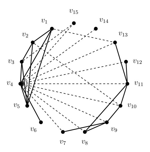
Figure 4: This is the partial 2-coloring C of K15 described in the proof of Theorem 2. The solid edges are red and the dashed edges are blue.
Table 2 gives additional diagonal graph Ramsey numbers, which were previously unknown when [21] was published, and which are not found in the current mathematical literature. These new results were obtained using the computational methods described in Section 3 of this paper.
Table 2: Some new diagonal graph Ramsey numbers. The "Gxxx" labels in this table correspond to classification numbers used in [21].
| G136 | G137 | G139 | G140 | G141 | G143 |
|---|---|---|---|---|---|
| o o o o o o | o o o o o o | o o o o o o | o o o o o o | o o o o o o | o o o o o o |
| 12 | 11 | 11 | 11 | 11 | 11 |
| G144 | G145 | G147 | G148 | G149 | G150 |
| o o o o o o | o o o o o o | o o o o o o | o o o o o o | o o o o o o | o o o o o o |
| 12 | 11 | 11 | 11 | 11 | 13 |
| G151 | G153 | G154 | G603 | G606 | (4) C 4 |
| o o o o o o | o o o o o o | o o o o o o | o o o o o o o | o o o o o o o | o o o o o o o o |
| 11 | 12 | 11 | 15 | 15 | 11 |
5. Miscellany
While exploring various graph Ramsey theory problems with Mathematica, Cowen [8] proved the following theorem. This beautiful result is what originally motivated our research project.
Theorem E. (Cowen [8]). Suppose R(Ks, Kt) = n. Then, G = Kn − {uv} has a red/blue edge coloring where there is neither a red Ks nor a blue Kt .
To conclude this paper, we extend Theorem E to r colors.
Theorem 3. Suppose R(Kx1 , Kx2 , . . . , Kxk ) = n. Then, G = Kn − {uv} has an r-coloring of the edges where no monochromatic Kxi exist in G.
Proof. Let G = Kn − {uv}. Since G − {u} is Kn−1, it has an r-coloring of the edges where no monochromatic Kxi exist in G. To complete the coloring of G, we color an edge ux, x ∈ V \{u, v} using the color of edge vx. We now claim that no monochromatic Kxi exist in G. Suppose (to the contrary) a monochromatic Kxi exists in G. Then, Kxi does not contain both u and v. Without loss of generality, u /∈ Kxi . Then, Kxi is a monochromatic subgraph of G − {u}. This gives a desired contradiction and establishes the claim.
References
- [1] S.A. Burr, Generalized Ramsey theory for graphs A survey, Graphs and Combinatorics, Springer-Verlag, Berlin, 1974, pp. 52-75.
- [2] S.A. Burr, A survey of noncomplete Ramsey theory for graphs, Ann. New York Acad. Sci 328 (1979), 58-75.
- [3] S.A. Burr and P. Erdos, Extremal Ramsey theory for graphs, ˝ Utilitas Mathematica 9 (1976), 247-258.
- [4] G. Chartrand and P. Zhang, New directions in Ramsey theory, Discrete Math. Lett 6 (2021), 84-96.
- [5] V. Chvatal and F. Harary, Generalized Ramsey theory for graphs, III: small off-diagonal ´ numbers, Pacific Journal of Mathematics 41 (1972), 335-345.
- [6] V. Chvatal and F. Harary, Generalized Ramsey theory for graphs, I: diagonal numbers, ´ Periodica Mathematica Hungarica 3 (1973), 115-124.
- [7] D. Conlon, A new upper bound for diagonal Ramsey numbers, Ann. of Math. (2) 170(2) (2009), 941-960.
- [8] R. Cowen, Deleting edges from Ramsey minimal examples, Amer. Math. Monthly 122(7) (2015), 681-683.
- [9] R. Cowen, Using Boolean computation to solve some problems from Ramsey theory, The Mathematica Journal, 2013. dx.doi.org/doi:10.3888/tmj.15-10.
- [10] C. Dalfo and M.A. Fiol, Graphs, friends and acquaintances, ´ Electron. J. Graph Theory Appl 6(2) (2018), 282-305.
- [11] H.B. Enderton, A Mathematical Introduction to Logic, Second Edition. Academic Press, 2001.
- [12] R. Graham and S. Butler, Rudiments of Ramsey Theory, Second Edition. CBMS Regional Conference Series in Mathematics 123. American Mathematical Society, Providence, R.I., 2015.
- [13] R. Graham, B. Rothschild, and J. Spencer, Ramsey Theory, Second Edition, Wiley, 2013.
- [14] J.W. Grossman, Some Ramsey numbers of unicyclic graphs, Ars Combin 8 (1979), 59-63.
- [15] C.J. Jayawardene, Diagonal Ramsey numbers in multipartite graphs related to stars, Electron. J. Graph Theory Appl 10(1) (2022), 227-237.
- [16] B.M. Landman and A. Robertson, Ramsey Theory on the Integers, Second Edition. Student Mathematical Library 73, American Mathematical Society, Providence, R.I., 2014.
- [17] C. Magnant and P.S. Nowbandegani, Topics in Gallai-Ramsey Theory, Springer International Publishing, 2020.
- [18] B.D. McKay and A. Piperno, Practical graph isomorphism, II. J. Symbolic Computation 60 (2013), 94-112.
- [19] S.P. Radziszowski, Small Ramsey numbers, Elect. J. Combin. 16 (2021), #DS1.
- [20] F.P. Ramsey, On a problem of formal logic, Proc. London Math. Soc. (2) 30(4) (1929), 264- 286.
- [21] R.C. Read and R.J. Wilson, An Atlas of Graphs, Oxford University Press, New York, 1998.
- [22] A. Robertson, Fundamentals of Ramsey Theory, First Edition, Chapman and Hall/CRC, 2021.
- [23] V. Rosta, Ramsey theory applications, Elect. J. Combin. (2004), #DS13.
- [24] A. Sah, Diagonal Ramsey via effective quasirandomness, preprint (arXiv: 2005.09251v1).
- [25] A. Soifer, The Mathematical Coloring Book: Mathematics of Coloring and the Colorful Life of Its Creators, Springer, New York, 2009.
- [26] B. Sudakov, Recent developments in extremal combinatorics: Ramsey and Turan type prob- ´ lems, Proceedings of the International Congress of Mathematics. Volume IV, 2579-2606, Hindustan Book Agency, New Delhi, 2010.
- [27] D.B. West, Introduction to Graph Theory, 2nd Ed., Pearson, 2017.
- [28] Wolfram Research, Inc., Mathematica, Version 12.3.1, Champaign, IL (2021).
- [29] X. Xu, M. Liang, and H. Luo, Ramsey Theory: Unsolved Problems and Results, University of Science and Technology of China Press, De Gruyter, Berlin/Boston, 2018.
- [30] X. Xu and S.P. Radziszowski, On some open questions for Ramsey and Folkman numbers, Graph Theory: Favorite Conjectures and Open Problems. Volume 1, 43-62, Probl. Books in Math., Springer, 2016.