Jyoti Champanerkar^a , Aihua Li^b

^aDepartment of Mathematical Sciences, William Paterson Unviersity, New Jersey, USA ^bAihua Li, Department of Mathematics, Montclair State University, New Jersey, USA

champanerkarj@wpunj.edu, lia@montclair.edu

In this paper, we study the interlace polynomial of a special graph with n vertices, called 4nsnowflake graph. It is similar as the friendship graph Fⁿ of n vertices, which is made of n 3-cycles sharing one center vertex. In stead of 3-cycles, the 4n-snowflake graph Qⁿ is constructed by gluing n 4-cycles to one center vertex. We describe certain properties of such graphs, provide recursive and explicit formulas for the interlace polynomials, and give some properties of such polynomials such as special values and patterns for certain coefficients.

Keywords: interlace polynomial, cycle graph, snowflake graph

Mathematics Subject Classification: 05C31, 05C50

DOI: 10.5614/ejgta.2023.11.1.14

1. Introduction

History and Background

Graph polynomials have been studied and applied to characterize certain properties of the considered graphs. Two well-known polynomials are Tutte and Martin polynomials [6],[7]. The concept of interlace polynomial first appeared along with a study of Euler circuits of undirected 4-regular graphs and the transformations [4]. Arratia, Bollobas, Coppersmith, and Sorkin [3] in- ´ troduced the interlace polynomial of a graph, a polynomial that represents the information gained from doing a toggling process on the graph.

The interlace polynomial of a graph gives important information about the graph, for example, the number of k-component circuit partitions, for any k ∈ N [3]. The interlace polynomials of

Received: 17 March 2022, Revised: 8 January 2023, Accepted: 29 January 2023.

certain special graphs, such as paths, cycles, stars, and complete graphs, were studied ([1, 3, 4].) Recently, ladder graphs, n-claw graphs, forest graphs, Friendship graphs, and butterfly graphs were studied ([2, 9, 10, 12].) Work has been done on multi-variate interlace polynomials as well, see [2, 8].

In this paper, we focus on snowflake graphs, which is similar as the Friendship graphs. In [12], Friendship graphs were studied. In the Friendship graph Fⁿ with n vertices, n 3-cycles share exactly one center vertex v. For the 4n-snowflake graphs, instead of 3-cycles, we glue n 4 cycles to one center vertex. We name it the 4n-snowflake graph. We describe certain properties of such graphs, provide recursive and explicit formulas for the interlace polynomials, and give some properties of the polynomials such as special values and patterns for certain coefficients.

Defining the pnterlace Polynomial

The interlace polynomial of a given simple graph G is recursively defined by Arratia, Bollobas, ´ and Sorkin in [3]. First, the interlace polynomial of the empty graph Eⁿ with n vertices is defined to be x n . For any non-empty undirected graph G, we first select one edge ab from G, where a and b are two adjacent vertices of G. We consider three special neighborhoods related to a and b: V^a = N(a) \ (N(b) ∪ {b}), V^b = N(b) \ (N(a) ∪ {a}), and Va,b = N(a) ∩ N(b). A toggling process on the edge ab is applied to G to create a "pivot" of G based on the neighborhoods for the two end vertices of a and b. This process creates a new graph Gab such that G and Gab have the same vertex set and for every pair of vertices u, v belonging to different neighborhoods Va, Vb, Vab shown above, uv is an edge of Gab if and only if uv is not an edge of G. The resulting graph Gab is called the pivot of G at ab. The interlace polynomial of a graph G is defined recursively by applying the pivot process.

Definition 1 (Interlace Polynomial). [3] Let G be any undirected graph with n vertices and ab be an edge of G. The interlace polynomial q(G, x) of G is defined by

\[q(G,x) = \begin{cases} x^n, & \text{if } E(G) = \emptyset, \\ q(G-a,x) + q(G^{ab} - b, x), & \text{if } ab \in E(G). \end{cases}\]

Figure 1. Toggling a graph on an edge ab

Arratia, Bollobas, and Sorkin in [3] showed that the interlace polynomial is well-defined, that ´ is, it is independent on the choice of the edge.

Existing results

Let n be a positive integer. Below we summarize known results of the interlace polynomials of several popular graphs such as cycles, paths, stars, complete graphs, and bipartite complete graphs.

Theorem 2. [3, 2, 12] The interlace polynomials of Pn, Cn, Sn, Kn, and Km,n are given below:

1. Let Pⁿ be the path with n edges. Then q(P0, x) = x, q(P1, x) = 2x, q(P2, x) = x ² + 2x, and q(P3, x) = 3x ² + 2x. For n ≥ 4,

\[q(P_n, x) = q(P_{n-1}, x) + xq(P_{n-2}, x).\]

2. Let Cⁿ be the cycle with n vertices (n ≥ 3). Then q(C3, x) = 4x, q(C4, x) = 3x ² + 2x, and for n ≥ 5,

\[q(C_n, x) = q(C_{n-2}, x) + q(P_{n-2}, x) + q(C_{n-4}, x).\]

3. Let Sⁿ be the star graph with n edges. Then q(S1, x) = 2, q(S2, x) = q(P2, x), and for x ≥ 3,

\[q(S_n, x) = x^n + x^{n-1} + \dots + x^2 + 2x;\]

• 4. q(Kn, x) = 2ⁿ−¹x, where Kⁿ is the complete graph with n vertices;
• 5. The complete bipartite graph Km,n satisfies

\[q(K_{m,n},x) = (1+x+\ldots+x^{m-1})(1+x+\ldots+x^{n-1})+x^m+x^n-1.\]

The interlace polynomial of a graph G may give some information about the graph G. Next we list some existing results about the interlace polynomial which reflect properties of the underlying graph.

Lemma 3. [3] Given the interlace polynomial q(G, x) of any undirected graph G. Denote the degree of q(G, x) by deg(q(G, x)). Then

• 1. If G is connected, then q(G, 0) = 0. That is, the constant term of q(G, x) is 0;
• 2. The degree of the lowest-degree term of q(G, x) is k(G), the number of connected components of G.
• 3. deg(q(G, x)) ≥ α(G), where α(G) is the independence number, i.e., the size of a maximum independent set.
• 4. Let µ(G) denote the size of a maximum matching (maximum set of independent edges) in a graph G. If G is a forest with n vertices, then deg(q(G, x)) = n − µ(G).

The 4n-Snowflake graphs and examples

In this research, we focus on a type of graph made by n 4-cycles, called 4n-snowflake graphs. Refer to Figure 2. The formal definition is given below.

Definition 4. Let Qⁿ be the graph by gluing n 4-cycles C⁴ at a common vertex (called the center vertex) such that every two of the n 4-cycles share exactly one vertex, the center vertex. We call Qⁿ the 4n-snowflake graph.

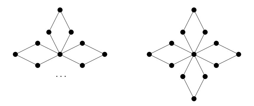
Figure 2. The Graph Qⁿ Made by n 4-Cycles (left) and Q⁴ (right)

The graph Qⁿ is similar to the Friendship Graph Fⁿ ([12]), which is the graph resulted by gluing n 3-cycles, instead of n 4-cycles. Obviously, the graph Q¹ = C4. In this paper, we study the properties of the graph Qⁿ and its interlace polynomial q(Qn, x). We give a useful recursive formula for q(Qn, x) and use it to investigate certain special values, coefficients, the properties of this polynomial. The adjacency matrix of Qⁿ and related matrices are studied. The interlace polynomial helps to describe the ranks of the matrices and some properties of the ground graph Qn.

2. Interlace Polynomial q(Qn, x) and Its Properties

First we list some basic graph theory properties about the graph Qn. We skip the proof because it is straightforward.

Lemma 5. Let n ≥ 1. Consider the graph Qⁿ = (V (Qn), E(Qn)) defined before. Then

• 1. |V (Qn)| = 3n + 1 and |E(Qn)| = 4n.
• 2. The degree sequence of Qⁿ is 2n, 2, . . . , 2 | {z } 3n copies.
• 3. Qⁿ has exactly one cut vertex, the center vertex of degree 2n.
• 4. The independence number of Qⁿ is α(Qn) = 2n.
• 5. The size of a maximal matching of Qⁿ is µ(Qn) = n + 1.

Since Q¹ = C4, the interlace polynomial q(Q1, x) = q(C4, x) = 3x ² + 2x. For n = 2, we decompose the graph Q² by two toggling processes. The graph Q² and its pivot Qab 2 at the edge ab are shown in Figure 3. By toggling at the edge ab, we decompose Q² into the two graphs Q² − a and Qab ² − b shown in Figure 4. Thus, we have

\[q(Q_2, x) = q(Q_2 - a, x) + q(P_1, x)q(C_4, x).\]

We further toggle the graph Q² − a at the edge bu and then at the edge uc (see Figure 4). It results in

\[q(Q_2 - a, x) = x^2 q(P_2, x) + q(C_4, x) + xq(P_2, x).\]

Figure 3. (a) The Graph \(Q_2\); (b) \(Q_2^{ab}\)

By Theorem 2(1)(2), \(q(P_1, x) = 2x\), \(q(P_2, x) = x^2 + 2x\), and \(q(C_4, x) = 3x^2 + 2x\). Combining these formulas,

\[q(Q_2, x) = (2x+1)q(C_4, x) + (x^2 + x)q(P_2, x)\]
= \((2x+1)(3x^2 + 2x) + (x^2 + x)(x^2 + 2x)\)
= \(x^4 + 9x^3 + 9x^2 + 2x\).

Figure 4. (a) The Graph \(Q_2 - a\); (b) \(Q_2^{ab} - b\)

Next, we give a recursive formula for the interlace polynomial of \(Q_n\) for any positive integer n > 1. The process is very similar as the pivot process for \(Q_2\).

Theorem 6. For any integer n > 1,

\[q(\mathcal{Q}_n, x) = (2x+1)q(\mathcal{Q}_{n-1}, x) + x^n(x+1)(x+2)^{n-1}.\]

Proof. We fix an edge ab of \(Q_n\). The graph \(Q_n\) and the pivot \(Q_n^{ab}\) are show in Figure 5. We perform a similar toggling process on ab as shown for the graph \(Q_2\):

• 1. Toggling \(Q_n\) at ab to obtain two graphs \(Q_n a\) and \(Q_n^{ab} b\) (refer to Figure 6). Obviously, \(Q_n^{ab} b = P_1 \dot{\cup} Q_{n-1}\), the disjoint union of the path \(P_1\) and \(Q_{n-1}\). Thus \(q(Q_n^{ab} b, x) = 2xq(Q_{n-1}, x)\).
• 2. Toggling the graph \(Q_n a\) at the edge bu which decomposes the graph into \((Q_n a) b\) and the disjoint union of the empty graph \(E_2\) with n 1 copies of \(P_2\) (Figure 7). Thus,

\[q(Q_n - a, x) = q((Q_n - a) - b, x) + x^2 q(P_2, x)^{n-1}.\]

3. Similarly, toggling the graph \((Q_n - a) - b\) at the edge cu, we obtain the graph \(Q_{n-1}\) and the disjoint union of \(E_2\) with n-1 copies of \(P_2\).

The above procedure produces the recursive relation:

\[q(\mathcal{Q}_{n-1} - a, x) = q(\mathcal{Q}_{n-1}, x) + xq(P_2, x)^{n-1} + x^2q(P_2, x)^{n-1}.\]

Since \(P_2 = x^2 + 2x\) by Theorem 2, we obtain

\[q(\mathcal{Q}_n, x) = (2x+1)q(\mathcal{Q}_{n-1}, x) + x(x+1)(q(P_2, x))^{n-1}\]
= \((2x+1)q(\mathcal{Q}_{n-1}, x) + x^n(x+1)(x+2)^{n-1}\).

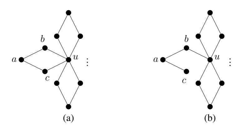
Figure 5. (a) The Graph \(Q_n\); (b) \(Q_n^{ab}\)

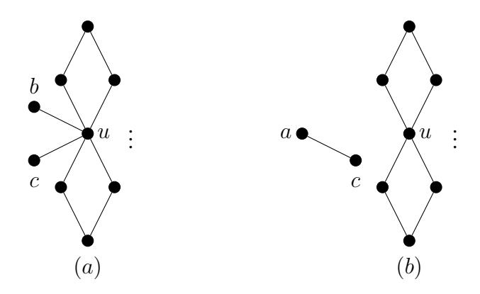
Figure 6. (a) The Graph \(Q_n - a\); (b) \(Q_n^{ab} - b = P_1 \dot{\cup} Q_{n-1}\)

Theorem 6 enables us to recursively describe the interlace polynomials \(q(Q_n, x)\) for all positive integers n. Below we show those for n = 1, 2, 3, 4, 5, 6, 7, 8. One can see some interesting patterns on the coefficients. They will be discussed later.

Example 1. 1. \[q(Q_1, x) = q(C_4, x) = 3x^2 + 2x\];

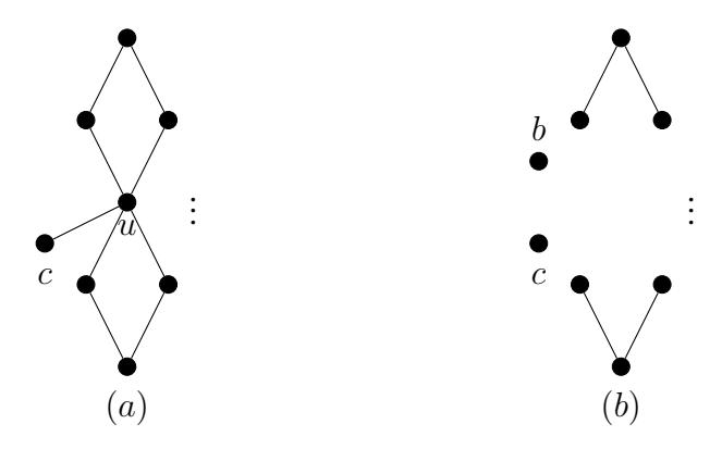
Figure 7. (a) \((Q_n - a) - b\); (b) \((Q_n - a)^{bu} - u = E_2 \dot{\cup} (n - 1) P_2\);

• 2. \(q(Q_2, x) = x^4 + 9x^3 + 9x^2 + 2x\);
• 3. \(q(Q_3, x) = x^6 + 7x^5 + 27x^4 + 31x^3 + 13x^2 + 2x\);
• 4. \(q(Q_4, x) = x^8 + 9x^7 + 33x^6 + 81x^5 + 97x^4 + 57x^3 + 17x^2 + 2x;\)
• 5. \(q(Q_5, x) = x^{10} + 11x^9 + 51x^8 + 131x^7 + 243x^6 + 291x^5 + 211x^4 + 91x^3 + 21x^2 + 2x;\)
• 6. \(q(Q_6, x) = x^{12} + 13x^{11} + 73x^{10} + 233x^9 + 473x^8 + 729x^7 + 857x^6 + 713x^5 + 393x^4 + 133x^3 + 25x^2 + 2x;\)
• 7. \(q(Q_7, x) = x^{14} + 15x^{13} + 99x^{12} + 379x^{11} + 939x^{10} + 1611x^9 + 2187x^8 + 2507x^7 + 2283x^6 + 1499x^5 + 659x^4 + 183x^3 + 29x^2 + 2x\).

Using the iterative formula given in Theorem 6 we develop an explicit formula for \(q(Q_n, x)\) at the value x = 1.

Theorem 7. For any positive integer n, \(q(Q_n, 1) = (2n + 3) \cdot 3^{n-1}\).

Proof. We prove the theorem by mathematical induction.

From Example 1, \(q(\mathcal{Q}_1, x) = 3x^2 + 2x\). So, \(q(\mathcal{Q}_1, 1) = 5 = (2 \cdot 1 + 3) \cdot 3^{1-1}\) and the formula is true for n = 1. For n > 1, we evaluate the recursive formula given in Theorem 6 at x = 1 which gives \(q(\mathcal{Q}_{n+1}, 1) = 3q(\mathcal{Q}_n, 1) + 2 \cdot 3^n\). By the induction hypothesis \(q(\mathcal{Q}_n, 1) = (2n + 3) \cdot 3^{n-1}\),

\[q(\mathcal{Q}_{n+1}, 1) = 3(2n+3) \cdot 3^{n-1} + 2 \cdot 3^n = (2(n+1)+3) \cdot 3^n.\]

Thus, the formula \(q(Q_n, 1)\) is true for all positive integers.

3. Explicit Formula for \(q(Q_n, x)\)

Theorem 7 gives an explicit formula for \(q(\mathcal{Q}_n, x)\) at x = 1. In this section, we develop an explicit formula for \(q(\mathcal{Q}_n, x)\) for every \(x \neq 1\).

Theorem 8. For \(x \neq 1\) and \(n \geq 1\),

\[q(\mathcal{Q}_n, x) = \frac{(x^2 - 2x)(2x+1)^n + x^{n+1}(x+2)^n}{x-1}.\]

Proof. It is by mathematical induction again. For n=1, the formula is true because by Example 1:

\[\frac{(x^2 - 2x)(2x+1) + x^2(x+2)}{x-1} = \frac{x(3x+2)(x-1)}{x-1} = 3x^2 + 2x = q(\mathcal{Q}_1, x).\]

Apply the induction hypothesis and the recursive formula given in Theorem 6 again,

\[q(\mathcal{Q}_{n+1}, x) = (2x+1)q(\mathcal{Q}_n, x) + x^{n+1}(x+1)(x+2)^n\] \[= (2x+1) \cdot \frac{(x^2 - 2x)(2x+1)^n + x^{n+1}(x+2)^n}{x-1} + x^{n+1}(x+1)(x+2)^n\] \[= \frac{(x^2 - 2x)(2x+1)^{n+1} + x^{n+2}(x+2)^{n+1}}{x-1}.\]

Many properties of \(q(\mathcal{Q}_n, x)\) can be developed from the above recursive formula and the explicit formula. It is known that some special values of the interlace polynomial can tell something about the underlying graph. The following proposition gives special values of \(q(\mathcal{Q}_n, x)\) at x = 2, -1, and 2. Formulas for the degree of the polynomial \(\mathcal{Q}_n\) and some coefficients are given as well.

Proposition 9. The interlace polynomial \(q(Q_n, x)\) \((n \ge 1)\) satisfies the following:

• 1. \(\deg(q(\mathcal{Q}_n, x)) = 2n\) and the leading coefficient of \(q(\mathcal{Q}_n, x)\) is 1 for n > 1.
• 2. The coefficient of the x-term is always 2 and the constant term is always 0. That is, \(q(Q_n, 0) = 0\) and \(\frac{d}{dx}q(Q_n, x)|_{x=0} = 2\);
• 3. \(q(Q_n, 2) = 2^{3n+1}\);
• 4. \(q(Q_n, -1) = (-1)^{n+1}\);
• 5. \(q(Q_n, -2) = 8(-3)^{n-1}\);
• 6. The parity of \(q(Q_n, x)\) is the same as that of x, that is, \(q(Q_n, x)\) is even if and only if x is even.

Proof. From Theorem 6, for n > 1 we have

\[q(\mathcal{Q}_n, x) = (2x+1)q(\mathcal{Q}_{n-1}, x) + x^n(x+1)(x+2)^{n-1}.\] (1)

From Theorems 7 and 8, we have

\[q(\mathcal{Q}_n, x) = \begin{cases} (2n+3)3^{n-1}, & \text{if } x = 1, \\ \frac{(x^2 - 2x)(2x+1)^n + x^{n+1}(x+2)^n}{x-1}, & \text{if } x \neq 1. \end{cases}\] (2)

We use equations (1) and (2) to prove the assertions stated in Proposition 9.

1. We apply mathematical induction on the number k>0 which is the number of copies of \(C_4\) in \(Q_k\). Since \(Q_1=C_4\), \(q(Q_1,x)=3x^2+2x\). Hence \(\deg(q(Q_1,x))=2\). Suppose \(\deg(q(Q_k,x))=2k\). We will prove the claim for \(Q_{k+1}\). From Equation (1),

\[q(\mathcal{Q}_{k+1}, x) = (2x+1)q(\mathcal{Q}_k, x) + x^{k+1}(x+1)(x+2)^k.\]

Obviously, deg(x ^k+1(x + 1)(x + 2)^k ) = 2k + 2. By the induction hypothesis, deg((2x + 1)q(Qk, x)) = 2k + 1 and the leading term of q(Qk+1, x) is x ²k+2. Hence, the degree of the polynomial q(Qk+1, x) is 2k + 2 = 2(k + 1) with leading coefficient 1. Thus by mathematical induction, the leading term of q(Qn, x) is x 2n and deg(q(Qn, x)) = 2n for every positive integer n;

• 2. Since q(Q1, x) = 3x ² + 2x, we see that the coefficient of the x-term is 2. Suppose that the coefficient of the x-term in q(Qk, x) is 2. We will prove the claim for q(Qk+1, x). Refer to Equation (1) again. Since the constant terms of q(Qk, x) is 0, the lowest degree term is 2x in q(Qk+1, x). Thus, by the principle of mathematical induction, the x-term in q(Qn, x) has coefficient 2 for all n ≥ 1.
• 3-5. The statements 3, 4, 5 can be shown by substituting 2, −1, −2 in the formula given in Theorem 8.
  • 6. By Theorem 7, it is true for n = 1. For n ̸= 1, note that in Equation (1), x n (x+ 1)(x+ 2)ⁿ−¹ is even for all integers x. Then the parity of q(Qn+1, x) is the same as that of q(Qn, x). However, q(Q1, x) is even if and only if x is even.

Next, we examine the coefficients of q(Qn, x). Since the degree of q(Qn, x) is 2n and the constant is 0, we write

\[q(\mathcal{Q}_n, x) = a_{n,(2n)}x^{2n} + a_{n,(2n-1)}x^{2n-1} + \dots + a_{n,2}x^2 + a_{n,1}x\]\[= \sum_{k=1}^{2n} a_{n,k}x^k.\]

From the previous results, an,¹ = 2, an,2ⁿ = 1. To obtain the other coefficients of q(Qn, x), we introduce another function fn(x):

\[f_n(x) = (x^2 - 2x)(2x+1)^n + x^{n+1}(x+2)^n.\]

By Theorem 8, for x ̸= 1, fn(x) = (x−1)q(Qn, x). Assume the coefficient of x k for fn(x) is bn,k, that is,

\[f_n(x) = \sum_{k=1}^{2n+1} b_{n,k} x^k = (x-1)q(\mathcal{Q}_n, x).\]

We now describe the coefficients of fn(x).

Theorem 10. Let n ≥ 4 and k ≥ 1. Then

\[b_{n,1}=-2, \quad b_{n,2}=1-4n, \quad b_{n,(2n+1)}=1, \quad b_{n,n+1}=2^{n-1}(n-2), \\ b_{n,n+2}=2^{n-1}(n+2), \quad \textit{and furthermore,}\]

\[b_{n,k} = \begin{cases} \binom{n+1}{k-1} \cdot \frac{2^{k-2}(5k-4n-9)}{n+1}, & \text{if } 3 \le k \le n, \\ \binom{n}{2n+1-k} \cdot 2^{2n+1-k}, & \text{if } n+3 \le k \le 2n. \end{cases}\]

Proof. Assume n ≥ 4. By binomial expansion,

\[f_{n}(x) = (x^{2} - 2x)(2x + 1)^{n} + x^{n+1}(x + 2)^{n}\] \[= \sum_{j=0}^{n} \binom{n}{j} 2^{j} x^{j+2} - \sum_{j=0}^{n} \binom{n}{j} 2^{j+1} x^{j+1} + \sum_{j=0}^{n} \binom{n}{j} 2^{n-j} x^{n+j+1}\] \[= \sum_{k=2}^{n+1} \left[ \binom{n}{k-2} 2^{k-2} - \binom{n}{k-1} 2^{k} \right] x^{k} + 2^{n} x^{n+2}\] \[+ \sum_{k=n+1}^{2n+1} \binom{n}{2n+1-k} 2^{2n+1-k} x^{k} - 2x\] \[= x^{2n+1} + \sum_{k=n+3}^{2n} \binom{n}{k-n-1} \cdot 2^{2n+1-k} \cdot x^{k}\] \[+ 2^{n-1}(n+2)x^{n+2} + 2^{n-1}(n-2)x^{n+1}\] \[+ \sum_{k=3}^{n} \binom{n+1}{k-1} \cdot \frac{2^{k-2}(5k-4n-9)}{n+1} x^{k} + (1+4n)x^{2} - 2x.\]

Thus we obtain the expression for every coefficient bn,k as stated in the Theorem. Note that for 3 ≤ k ≤ n, it is straightforward to check that

\[\binom{n}{k-2}2^{k-2} - \binom{n}{k-1}2^k = \binom{n+1}{k-1} \cdot \frac{2^{k-2}(5k-4n-9)}{n+1}.\]

The relationship between the coefficients of f(x) and q(Qn, x) is given by

Lemma 11. Let n, k be positive integers with k ≤ 2n.

• (1) bn,¹ = −an,¹ = −2 and bn,2n+1 = an,2ⁿ = 1;
• (2) If 2 ≤ k ≤ 2n, bn,k = an, k−¹ − an,k.
• (3) For any 1 ≤ k ≤ 2n, an,k = − P^{k j}=1 bn,j .
• (4) P²n+1 ^j=1 bn,j = 0.

Proof. The claims (1) and (2) are directly from the formula fn(x) = (x − 1)q(Qn, x). From (2), for 1 ≤ k ≤ 2n,

\[\sum_{j=1}^{k} b_{n,j} = -a_{n,1} + (a_{n,1} - a_{n,2}) + (a_{n,2} - a_{n,3}) + \dots + (a_{n,k-1} - a_{n,k}) = -a_{n,k}.\]

It proves (3). For (4), applying (1) and (3).

The above lemma and the Theorem 10 can help in developing the explicit formula for each coefficient an,k of the polynomial q(Qn, x). Now we discuss these coefficients.

Theorem 12. For \(n \geq 1\), \(q(Q_n, x)\) can be expressed as

1.

\[q(Q_n, x) = x^{2n} - \sum_{k=2}^{2n-1} \left(\sum_{j=1}^k b_{n,j}\right) x^k + 2x.\]

2.

\[q(\mathcal{Q}_n, x) = x^{2n} + 2x^{2n-1} + \sum_{k=n}^{2n-1} {n \choose k-n} \cdot \frac{k \cdot 2^{2n-k-1}}{n} \cdot x^k + \sum_{k=2}^{2n-2} (2a_{n-1, k-1} + a_{n-1, k})x^k + 2x.\]

Proof. (1) is directly from Lemma 11(3). For (2), by Theorem 6,

\[q(\mathcal{Q}_n, x) = (2x+1)q(Q_{n-1}, x) + x^n(x+1)(x+2)^{n-1}.\]

Recall that \(q(Q_{n-1}, x) = \sum_{k=1}^{2n-2} a_{n-1,k} x^k\) and the leading coefficient is \(a_{n-1,2(n-1)} = 1\). The first part of \(q(Q_{n-1}, x)\) can be expressed as:

\[(2x+1)q(\mathcal{Q}_{n-1},x) = \sum_{k=1}^{2n-2} 2a_{n-1,k}x^{k+1} + \sum_{k=1}^{2n-2} a_{n-1,k}x^k\]\[= 2x^{2n-1} + \sum_{k=2}^{2n-2} (2a_{n-1,k-1} + a_{n-1,k})x^k + 2x.\]

By the binomial expansion formula, the second part of \(q(Q_{n-1}, x)\) can be written as

\[x^{n}(x+1)(x+2)^{n-1} = x^{n+1}(x+2)^{n-1} + x^{n}(x+2)^{n-1}\] \[= \sum_{j=0}^{n-1} \binom{n-1}{j} 2^{n-j-1} x^{n+j+1} + \sum_{j=0}^{n-1} \binom{n-1}{j} 2^{n-j-1} x^{n+j}\] \[= x^{2n} + \sum_{j=1}^{n-1} \left[ \binom{n-1}{j-1} 2^{n-j} + \binom{n-1}{j} 2^{n-j-1} \right] x^{n+j} + 2^{n-1} x^{n}\] \[= x^{2n} + \sum_{j=1}^{n-1} \binom{n}{j} \frac{n+j}{n} \cdot 2^{n-j-1} x^{n+j} + 2^{n-1} x^{n}\] \[= x^{2n} + \sum_{k=n}^{2n-1} \binom{n}{k-n} \cdot \frac{k \cdot 2^{2n-k-1}}{n} \cdot x^{k}.\]

Combining all the above, we obtain the desired expression for \(q(Q_n, x)\).

Applying Theorems 12 and 10, we can describe the coefficients \(a_{n,k}\) as follows:

Theorem 13. For any integer n ≥ 4,

• 1. The second leading coefficient of q(Qn, x) is an,(2n−1) = 2n + 1.
• 2. The coefficient of the x ⁿ+1-term in q(Qn, x) is an. n+1 = 3ⁿ ;
• 3. The coefficient of the x n -term is an, n = 3ⁿ + (n − 2)2ⁿ−¹ .
• 4. For 2 ≤ k ≤ n − 1, an, k = 2an−1, k−¹ + an−1, k.
• 5. For n + 1 ≤ k ≤ 2n − 2,

\[a_{n,k} = 2a_{n-1,k-1} + a_{n-1,k} + \binom{n}{k-n} \cdot \frac{k \cdot 2^{2n-k-1}}{n}.\]

Proof. Throughout the proof, we need apply Theorems 12,10, and Lemma 11.

1. The second leading coefficient is given by

\[a_{n,2n-1} = b_{n,(2n)} + a_{n,(2n)} = \binom{n}{2n-n-1} \cdot 2^{2n+1-2n} + 1 = 2n+1.\]

2. By Lemma 11 and Theorem 10, an−1, n+1 = an−1, n − bn−1, n+1 = an−1, n − 2 n−2 (n + 1). Then

\[a_{n,n+1} = \binom{n}{1} \frac{n+1}{n} \cdot 2^{n-2} + 2a_{n-1,n} + a_{n-1,n+1}\] \[= (n+1)2^{n-2} + 2a_{n-1,n} + a_{n-1,n} - b_{n-1,n+1}\] \[= (n+1)2^{n-2} + 3a_{n-1,n} - (n+1)2^{n-2} = 3a_{n-1,n}.\]

Example 1 shows that a3, ⁴ = 3³ = 27. Then for any n ≥ 4,

\[a_{n,n+1} = 3a_{n-1,n} = 3^2 \cdot a_{n-2,n-1} = \dots = 3^{n-3}a_{3,4} = 3^{n-3} \cdot 3^3 = 3^n.\]

• 3. Similarly as in the above proof, an, n = an, n+1 + bn, n+1. Applying the result from the above part 4 and Theorem 10, we have an, n = 3ⁿ + (n − 2)2ⁿ−¹ .
• 4. (4) and (5) are straightforward. We skip the proof.

Corollary 14. For any integer n ≥ 4,

• 1. The third leading coefficient of q(Qn, x) is an, (2n−2) = 2n ² + 1;
• 2. Coefficients for x 2 and x 3 are respectively an,² = 4n + 1 and an,³ = 4n ² − 2n + 1.

Proof. 1. By Lemma 11 and Theorem 10,

\[a_{n,2n-2} = b_{n,(2n-1)} + a_{n,(2n-1)} = \binom{n}{n-2} \cdot 2^2 + (2n+1) = 2n^2 + 1.\]

2. The coefficients of \(x^2\) and \(x^3\) are obtained by the follow the relations:

\[\begin{array}{rcl} a_{n,2} & = & a_{n,1} - b_{n,2} = 2 - (1 - 4n) = 4n + 1 & \text{and then} \\ a_{n,3} & = & a_{n,2} - b_{n,3} = 4n + 1 - \binom{n+1}{2} \cdot \frac{2(6-4n)}{n+1} = 4n^2 - 2n + 1. \end{array}\]

We observe that the coefficient sequence \((a_{n,k})_{k=1}^{2n}\) seems to be one mode with a maximal value around in the middle \((a_{n,n})\) and all coefficients are odd except for the leading one. For example,

\[(a_{5,k})_{k=1}^{k=10} = (2, 21, 91, 211, 291, 243, 131, 51, 11, 1).\]

We claim that the coefficient sequence is one mode, but the maximum does not necessarily occur in the middle. Also, the leading coefficient is the only even coefficient. Consider the sequence \((a_{n,k})_{k=1}^{2n}\), representing the coefficients of the polynomial \(q(\mathcal{Q}_n,x)\).

Proposition 15. Consider the sequence \((a_{n,k})_{k=1}^{2n}\) with \(n \geq 7\). Denote \(r_n = \lfloor \frac{4n+9}{5} \rfloor\).

1. \((a_{n,k})_{k=1}^{2n}\) is increasing from k=1 to \(k=r_n\) and then decreasing from \(k=R_n\) to k=2n. That is,

\[2 = a_{n,1} < \cdots < a_{n,n-1} < a_{n,r_n} > a_{n,n+1} > \cdots > a_{n,2n} = 1.\]

• 2. \(\max(a_{n,k})_{k=1}^{2n} = a_{n,n} \iff n \in \{7, 8, 9\}.\)
• 3. \(a_{n,1} = 2\) and \(a_{n,k}\) is odd for all k with 2 < k < 2n.

Proof. (1) By Theorem 13 and Corollary 14,

\[\begin{array}{rcl} a_{n,2n} & = & 1 < a_{n,\,2n-1} = 2n+1 < a_{n,\,2n-2} = 2n^2+1, \\ a_{n,\,n+1} & = & 3^n < a_{n,\,n} = 3^n+(n-2)2^{n-1}, \quad \text{and} \\ a_{n,3} & = & 4n^2-2n+1 > a_{n,2} = 4n+1 > a_{n,1} = 2. \end{array}\]

It remains to show that \(a_{n,k} < a_{n,k-1}\) for \(n+1 \le k \le 2n-3\) and \(a_{n,k} > a_{n,k-1}\) for \(3 \le k \le n-1\). By Lemma 11(1), \(a_{n,k}=a_{n,k-1}-b_{n,k}\) for \(2 \le k \le 2n\) and by Theorem 10, \(b_{n,k}>0\) for \(n+1 \le k \le 2n+1\). Thus \(a_{n,k} < a_{n,k-1}\) is true for \(n+1 \le k \le 2n-2\).

For \(3 \le k \le n\), since \(a_{n,k} = a_{n,k-1} - b_{n,k}\), \(a_{n,k} \ge a_{n,k-1}\) if and only if \(b_{n,k} \le 0\). While, by Theorem 10,

\[b_{n,k} \le 0 \iff 5x - 4n - 9 \le 0 \iff k \le \frac{4n + 9}{5} \iff k \le r_n.\]

Thus, \(a_{n,3} \leq a_{n,4} \leq \cdots \leq a_{n,r_n}\) and \(a_{n,r_n} \geq a_{n,k+1} \cdots \geq a_{n,n}\). For (2), note that \(n \leq \frac{4n+9}{5} < n+1 \iff 5n \leq 4n+9 < 5n+5 \iff n \leq 9\) and n > 4. Thus, if and only if n = 7, 8, or 9, the peak value occurs at the middle.

(3) is immediately from Theorem 13(4).

4. The Rank of a Related Matrix

In graph theory, the adjacency matrix of a given graph is used to describe the adjacency of the vertices and some connectivity properties. In particular, certain operations on the adjacency matrix help in counting the numbers of paths and cycles in the graph. In [5], Balister, Bollóbas, Cutler, and Peabody gave an explicit formula for the interlace polynomial of a graph at x = -1 involving the rank of the adjacency matrix plus the identity matrix modulo 2.

Theorem 16. [5] Let A be the adjacency matrix of a graph G with m vertices and let r = rank(A + I) modulo 2, where I is the \(m \times m\) identity matrix. Then

\[q(G,-1) = (-1)^m (-2)^{m-r}\].

Recall that the graph \(\mathcal{Q}_n\) has 3n+1 vertices. Denote the adjacency matrix of \(\mathcal{Q}_n\) by \(A_{3n+1}\) and let \(B_{3n+1}=A_{3n+1}+I_{3n+1}\), where \(I_{3n+1}\) is the \((3n+1)\times(3n+1)\) identity matrix. In this section, we examine the adjacency matrix \(A_{3n+1}\) and \(B_{3n+1}\). We apply the above result to determine the rank of the adjacency matrix \(B_{3n+1}\).

Example 2. Consider the graph \(Q_1 = C_4\). The adjacency matrix \(A_4\) of \(Q_1\) and \(B_4 = A_4 + I\) are shown below:

\[A_4 = \left[ \begin{array}{cccc} 0 & 1 & 0 & 1 \ 1 & 0 & 1 & 0 \ 0 & 1 & 0 & 1 \ 1 & 0 & 1 & 0 \end{array} \right] \quad \text{and} \quad B_4 = A_4 + I = \left[ \begin{array}{cccc} 1 & 1 & 0 & 1 \ 1 & 1 & 1 & 0 \ 0 & 1 & 1 & 1 \ 1 & 0 & 1 & 1 \end{array} \right].\]

one can easily check that modulo 2, \(det(B_4) = 1 \neq 0 \Longrightarrow rank(B_4) = 4\),, that is, \(B_4\) is of full rank modulo 2.

Refer to the graph of \(Q_n\) with vertices labeled as follows:

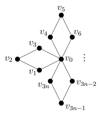
Figure 8. The Graph \(Q_n\) with labeled vertices

Assume the \(i^{\text{th}}\) row of the adjacency matrix \(A_{3n+1}\) represents the vertex \(v_i\) (\(i=0,1,\ldots,3n+1\)). The \(1\times 3\) matrix C=[1,0,1] occurs repeatedly as a sub-matrix of \(A_{3n+1}\). Then the first row

of \(A_{3n+1}\), representing \(v_0\), is \([1, C, C, \ldots, C]\) with n copies of C. For \(1 \le k \le n\), the adjacency matrix for the induced subgraph by \(v_{3k-2}, v_{3k-2}, v_{3k}\) is given by

\[M_A = \left[ \begin{array}{ccc} 0 & 1 & 0 \ 1 & 0 & 1 \ 0 & 1 & 0 \end{array} \right] \quad \text{and} \quad M_B = M_A + I_3 = \left[ \begin{array}{ccc} 1 & 1 & 0 \ 1 & 1 & 1 \ 0 & 1 & 1 \end{array} \right],\]

where \(I_3\) is the \(3 \times 3\) identity matrix. We now give the structures of the matrices \(A_{3n+1}\) and \(B_{3n+1}\):

Lemma 17. Let n be any positive integer and \(A_{3n+1}\), \(B_{3n+1}\), C, \(M_A\), \(M_B\) be as above. Then the two \((3n+1) \times (3n+1)\) matrices \(A_{3n+1}\) and \(B_{3n+1}\) are structured below:

\[A_{3n+1} = \begin{bmatrix} 1 & C & \cdots & C \\ C^T & M_A & & \\ \vdots & & \ddots & \\ C^T & & & M_A \end{bmatrix} \text{ and } B_{3n+1} = \begin{bmatrix} 1 & C & \cdots & C \\ C^T & M_B & & \\ \vdots & & \ddots & \\ C^T & & & M_B \end{bmatrix},\]

where the empty places are occupied by 0's.

As an application of the result for interlace polynomials stated in Theorem 16, we claim that for every positive integer n, the matrix \(B_{3n+1}\) is of full rank modulo 2.

Theorem 18. For any positive integer n, the matrix \(B_{3n+1}\) is of full rank modulo 2. That is, \(rank(B_{3n+1}) = 3n + 1 \mod 2\).

Proof. Let \(r_n\) be the rank of \(B_{3n+1}\) modulo 2. By Proposition 13, \(q(\mathcal{Q}_n, -1) = (-1)^{n+1}\). But By Theorem 16, the value \(q(\mathcal{Q}_n, -1) = (-1)^{3n+1}(-2)^{(3n+1)-r_n}\) modulo 2. Thus

\[(-1)^{3n+1}(-2)^{(3n+1)-r_n} = (-1)^{n+1} \Longrightarrow (-2)^{(3n+1)-r_n} = 1 \Longrightarrow\]

\[r_n = 3n + 1\]. Therefore, \(B_{3n+1}\) is of full rank (mod 2).

Of course, the above result can be achieved by the traditional linear algebra method through elementary row operations. But the process is more complicated. We sketch the process briefly.

Refer to Example 2. Since the matrix \(A_4\) is of full rank, it is row equivalent to \(I_4\). By applying the same row reduction that reduces \(A_4\) to \(I_4\), we obtain the matrix below which is row equivalent \((\sim)\) to \(B_{3n+1}\):

\[B_{3n+1} \sim \begin{bmatrix} 1 & C & C & \cdots & \cdots & C \\ \mathbf{0} & I_3 & * & \cdots & \cdots & * \\ C^T & \mathbf{0} & M_B & * & \cdots & * \\ \vdots & \vdots & \ddots & \ddots & & \vdots \\ C^T & \mathbf{0} & & \ddots & M_B & * \\ C^T & \mathbf{0} & \cdots & \cdots & \mathbf{0} & M_B \end{bmatrix}_{(3n+1)\times(3n+1)} = B'_{3n+1},\]

Using the number 1 in the (1,1) position of \(B_{3n+1}'\), we can perform elementary row operations to make the resulting matrix having 0 in the (i,1) positions for all i>1. Similarly, by performing corresponding elementary column operations, we can reduce the matrix into one with 0 in all of the (1,j) positions. That is, by multiplying an invertible matrix A from left and some invertible matrix A' from right, we obtain

\[AB_{3n+1}A' = \begin{bmatrix} 1 & \mathbf{0} & \mathbf{0} & \cdots & \cdots & \mathbf{0} \\ \mathbf{0} & I_3 & * & \cdots & \cdots & * \\ \mathbf{0} & \mathbf{0} & M_B & * & \cdots & * \\ \vdots & \vdots & \ddots & \ddots & & \vdots \\ \mathbf{0} & \mathbf{0} & & \ddots & M_B & * \\ \mathbf{0} & \mathbf{0} & \cdots & \cdots & \mathbf{0} & M_B \end{bmatrix}_{(3n+1)\times(3n+1)} = B''_{3n+1}.\]

Since \(M_B\) a 3 \(\times\) 3 matrix of full tank, the rank of \(B_{3n+1}''\) is 3n+1 and so does that of \(B_{3n+1}\). Certainly the method using the interlace polynomial of \(\mathcal{Q}_n\) to determine the rank of \(B_{3n+1}\) is easier (Theorem 18). It is nice to see an application of a graph theory result in solving a linear algebra problem.

Acknowledgement

Part of this work was supported by the National Science Foundation Grant No. 2028011.

References

• [1] M. Aigner and H. Holst, Interlace polynomials, Linear Algebra Appl. 377 (2004), 11–30.
• [2] C. Anderson, J. Cutler, A.J. Radcliffe, and L. Traldi, On the Interlace Polynomials of Forests, Discrete Mathematics, 310(1) (2010), 31–36.
• [3] R. Arratia, B. Bollobas, and G. Sorkin, The interlace polynomial of a graph, J. Combin. Theory 92 (2004), 199–233.
• [4] R. Arratia, B. Bollobas, D. Coppersmith, and G.B. Sorkin, Euler Circuits and DNA Sequencing by Hybridization, Discrete Appl. Math. 104(1-3) (2000), 63–96.
• [5] P.N. Balister, B. Bollobas, J. Cutler, and L. Pebody, The interlace polynomial of graphs at -1, Europ. J. Combinatorics 23 (2002), 761–767.
• [6] A. Bouchet, Graph polynomials derived from Tutte's Martin polynomials, Discrete Math. 302 (2005), 32–38.
• [7] J.A. Ellis-Monaghan, Identities for circuit partition polynomials, with applications to the Tutte polynomial, Advances in Applied Mathematics 32 (2004), 188–197.
• [8] J.A. Ellis-Monaghan and I. Sarmiento, Distance hereditary graphs and the interlace polynomial, Combinatorics, Probability and Computing 16 (2007), 947–973.

• [9] R. Glantz and M. Pelillo, Graph polynomials from principal pivoting, Discrete Math. 306 (2006), 3253–3266.
• [10] A. Li and Q. Wu, Interlace polynomials of ladder Graphs, Journal of Combinatorics, Information & System Sciences 35(1-2) (2010), 261–273.
• [11] S. Nomani and A. Li, Interlace polynomials of n-claw graphs, Journal of Combin. Math. Combin. Comput. 88 (2014), 111–122.
• [12] C.E. Turner and A. Li, Interlace polynomials of friendship graphs, Electron. J. Graph Theory Appl. 6(2) (2018), 269–281.
• [13] C. Uiyyasathian and S. Saduakdee, Perfect Glued Graphs at Complete Clones, Journal of Mathematics Research 1(1) (2009), 25–30.