Bryan Freyberg^a , Melissa Keranen^b

^aDepartment of Mathematics and Statistics, University of Minnesota Duluth, Duluth, USA

A k-regular d-handicap tournament is an incomplete tournament in which n teams, ranked according to the natural numbers, play exactly k < n − 1 different teams exactly once and the strength of schedule of the i th ranked team is d more than the (i − 1)st ranked team for some d ≥ 1. That is, strength of schedules increase arithmetically by d with strength of team. A d-handicap distance antimagic labeling of a graph G = (V, E) of order n is a bijection ℓ : V → {1, 2, . . . , n} with induced weight function w(xi) = P xj∈N(xi) l(x^j ) such that ℓ(xi) = i and the sequence of weights

w(x1), w(x2), . . . , w(xn) forms an arithmetic sequence with difference d ≥ 1. A graph G which admits such a labeling is called a d-handicap graph.

Constructing a k-regular d-handicap tournament on n teams is equivalent to finding a k-regular d-handicap graph of order n. For d = 1 and n even, the existence has recently been completely settled for all pairs (n, k), and some results are known for d = 2. For d > 2, the only known result is restricted to the case where n is divisible by 2 d+2 . In this paper, we construct infinite families of d-handicap graphs where the order is not restricted to a power of 2.

Keywords: Graph labeling, distance antimagic labeling, d-handicap labeling Mathematics Subject Classification : 05C70, 05C76, 05C78

DOI: 10.5614/ejgta.2023.11.1.7

1. Motivation

When scheduling a tournament, it is a common practice to use the rankings of the teams from the previous season, or some other source to determine the list of opponents for each team. A

Received: 22 November 2019, Revised: 6 January 2023, Accepted: 29 January 2023.

^bDepartment of Mathematical Sciences, Michigan Technological University, Houghton, USA frey0031@d.umn.edu, msjukuri@mtu.edu

tournament may be modeled with a graph in the most natural way; each team is represented with a vertex and two vertices are adjacent if and only if the corresponding two teams play each other.

Suppose we have n teams ranked with the first n natural numbers and let i be the team ranked i. For \(i \in \{1, 2, \ldots, n\}\), let w(i) represent the sum of the rankings of all opponents of team i. We call w the strength of schedule. In a round-robin tournament (a tournament in which every team plays all other teams), \(w(i) = \frac{n(n+1)}{2} - i\) for each i. This means the strengths of schedules form an arithmetic progression with difference -1 in a round-robin tournament. Therefore, the weakest team has the most difficult strength of schedule while the strongest team has the weakest strength of schedule. Clearly, the strongest team is most likely to benefit from this kind of tournament. This motivates the following questions that are of interest for both tournament scheduling reasons and purely graph theoretic reasons.

• Can we design a tournament with less games, but maintain the same weight structure as the round-robin tournament?
• Can we design a tournament so each team has the same strength of schedule?
• Can we turn things around so that the weakest team has the weakest strength of schedule?

Clearly, to address these questions, one must consider only incomplete tournaments, that is tournaments in which each team plays exactly k < n - 1 other teams (unless otherwise noted, it is assumed that all the tournaments discussed here are regular tournaments). A fair incomplete tournament is an incomplete tournament where the weights form an arithmetic progression with difference -1 as in a round-robin tournament. These tournaments address the first question above. See [7, 11] for results regarding fair incomplete tournaments.

Equalized incomplete tournaments address the second question above. An equalized incomplete tournament is an incomplete tournament such that \(w(i) = \mu\), for some constant \(\mu\), for every team i. The corresponding graph is called a distance magic graph. A distance magic labeling of a simple graph G = (V, E) of order n is a bijection \(f: V \to \{1, 2, \dots, n\}\) such that there exists an integer \(\mu\) called the magic constant, so that \(w(x) = \sum_{y \in N(x)} f(y) = \mu\) for all \(x \in V\). Here

The last question is addressed by a d-handicap tournament. A d-handicap distance antimagic labeling (or d-handicap labeling for short) of a graph G = (V, E) of order n is a bijection \(\ell : V \to \{1, 2, \ldots, n\}\) with induced weight function

\(N(x) = \{y | xy \in E\}\) represents the open neighborhood of x.

\[w(x_i) = \sum_{x_j \in N(x_i)} \ell(x_j),\]

such that \(\ell(x_i) = i\) and the sequence of weights \(w(x_1), w(x_2), \dots, w(x_n)\) forms an arithmetic sequence with constant difference \(d \geq 1\). If a graph G admits a d-handicap labeling, we say G is a d-handicap graph. If G is k-regular, then we say G corresponds to a k-regular d-handicap tournament, and we denote it by H(n, k, d).

A similar but less restrictive labeling has been considered by Arumugam and Kamatchi in [4]. An (a, d)-distance antimagic labeling of a graph G = (V, E) of order n is a bijection l:

V → {1, 2, . . . , n} such that the weights form the set {a, a + d, a + 2d, . . . , a + (n − 1)d} for some fixed integers a and d ≥ 0. Therefore, a d-handicap distance antimagic labeling is an (a, d) distance antimagic labeling, but the converse is not necessarily true. For a survey of distance magic and distance antimagic labelings, see [3]. The survey also provides a summary of the results regarding the tournaments we have discussed in this section.

In this paper we provide necessary conditions for the existence of d-handicap tournaments, H(n, k, d), and construct such tournaments for large classes of n and a wide range of regularities k, for every d ≥ 1. Our results subsume the complete characterizations of 1-handicap tournaments with n ≡ 0 (mod 8) and 2-handicap tournaments with n ≡ 0 (mod 16), which were proved respectively in [12, 8]. For larger d, our construction provides a nearly complete characterization for appropriate classes of n.

2. Tools

All graphs in this paper are simple, finite graphs. We use the notation V (G) to denote the vertex set of G and the notation E (G) to denote the edge set of G. If |V (G)| = n, we say the graph G has order n. The neighborhood of a vertex x ∈ V (G), denoted N(x) or N ^G(x), is the set of all vertices in V (G) adjacent to x. In order to simplify notation, we may sometimes refer to a vertex by its label. This should not cause any confusion since the labelings considered in this paper are bijections.

We use the notation xy to denote an edge between vertex x and vertex y and the notation x ∼ y to mean x is adjacent to y. Let Kn,m = [x1, x2, . . . , xⁿ | y1, y2,. . . , ym] denote the complete bipartite graph Kn,m with partite sets {x1, x2, . . . , xn} and {y1, y2, . . . , ym} . For two graphs G and H, we use the notation G + H to denote the union of graphs G and H. That is, V (G + H) = V (G) ∪ V (H) and E (G + H) = E(G) ∪ E(H). The complement of G is denoted by G.

The constructions used in this paper utilize two graph products. Given two graphs G and H, both products, the lexicographic product, G ◦ H, and the Cartesian product, G□H, have vertex set V (G) × V (H) and two vertices (g1, h1) and (g2, h2) are adjacent in

• G H if and only if g¹ ∼ g² in G or g¹ = g² and h¹ ∼ h² in H,
• G□H if and only if g¹ = g² and h¹ ∼ h² in H, or h¹ = h² and g¹ ∼ g² in G.

The lexicographic product G ◦ H has sometimes been called graph composition and has also been denoted G[H]. To construct the graph G ◦ H, the following informal description may be helpful. First, replace each vertex of G with an isomorphic copy of H. Then for every xy ∈ E(G), construct the complete bipartite graph K^|V (H)|,|^V (H)^| between the corresponding copies of H. For the graph G ◦ K2, we will refer to each pair of isolated vertices which replace a vertex of G as blown-up vertices. For a fixed vertex g of G, the subgraph of either of the above products induced by the set {(g, h) : h ∈ V (H)} is called an H-layer and is denoted H^g . Similarly, if h ∈ V (H) is fixed, then G^h , the subgraph induced by {(g, h) : g ∈ V (G)}, is a G-layer.

Circulant graphs are nice candidates for constructing tournaments since they are vertextransitive, regular, and can easily be manipulated to be more or less dense. Let S = {d1, d2, . . . , dm} and 1 ≤ d¹ < d² < · · · < d^m ≤ ^m 2 . We call S the connection set. Then

the circulant graph G = Cⁿ (S) is a graph with vertex set V (G) = {x0, x1, . . . , xn−1} and two vertices xⁱ and x^j are adjacent in G if and only if i − j ≡ d^k (mod n) for some k ∈ {1, 2, . . . , m}. Froncek and Cichacz in [5] showed certain classes of circulant graphs are distance magic. Figure 1 shows a distance magic labeling of C6(1, 2).

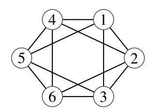
Figure 1. Distance magic labeling of C6(1, 2).

A 1-factor or perfect matching of a graph G is a union of disjoint edges xy ∈ E(G) such that every vertex v ∈ V (G) appears exactly once in the union. If for a graph G the edge set E (G) can be partitioned into a disjoint union of 1-factors, then we say G is 1-factorable or class 1.

Let S = {a, a+1, a+2, . . . , b} be a set of consecutive integers for integers a, b such that a ≤ b. If α, β ∈ S such that α + β = a + b, we will refer to the numbers α and β as S-complements, or simply complements if the set is clear from the context. It is obvious that if |S| is even, then S can be partitioned into complement pairs.

One of the primary ingredients for the constructions given in this paper are distance magic graphs. In particular, we are interested in regular distance magic graphs.

Theorem 2.1. (Vilfred [15]) Let d ≥ 1 be an odd integer. No d-regular graph is distance magic.

Froncek et al. proved the following in [11].

Theorem 2.2. (Froncek et al. [11]) For n even, an r-regular distance magic graph of order n exists if and only if 2 ≤ r ≤ n − 2, r ≡ 0 (mod 2), and either n ≡ 0 (mod 4) or r ≡ 0 (mod 4).

For regular graphs of odd order, the existence question is partially answered by the following result proved by Froncek in [7].

Theorem 2.3. (Froncek [7]) Let n be an odd integer and r = 2^s q with q > 1 odd and s ≥ 1. Then an r-regular distance magic graph of order n exists whenever r ≤ 2 7 (n − 2).

3. Necessary Conditions and Known Results

We begin this section by stating some necessary conditions.

Theorem 3.1. If a k-regular d-handicap graph of order n exists, then all of the following are true.

• (1) w(xi) = di + (k−d)(n+1) 2 , for all i ∈ {1, 2, . . . , n}.
• (2) If n is even, then k ≡ d (mod 2).

• (3) If n is odd, then k is even.
• (4) n ≥ 4d + 3.
• (5) d + 1 ≤ k ≤ n − d − 4, if n and d are odd and d ≥ 3.
• (6) d + 2 ≤ k ≤ n − d − 3, if n is odd and d is even.
• (7) d + 2 ≤ k ≤ n − d − 4, if n is even or d = 1.

Proof. Let G ∼= H (n, k, d) be given for some n, k, and d with d-handicap distance antimagic labeling l(xi) = i. Then w(xi) = µ + di for all i ∈ {1, 2, . . . , n} and some integer µ. Summing the weights, we have

\[w(G) = \sum_{i=1}^{n} w(x_i) = \mu n + d \sum_{i=1}^{n} i\]

and

\[w(G) = k \sum_{i=1}^{n} i,\]

since G is k-regular. Therefore,

\[\mu = \frac{k-d}{n} \sum_{i=1}^{n} i = \frac{(k-d)(n+1)}{2}.\]

If n is even, then k − d must be even (recall µ is an integer), which implies k ≡ d (mod 2). If n is odd, then k must be even by the handshaking lemma, so we have proven (1), (2), and (3).

To obtain the bounds (4) through (7), observe the weight of the vertex labeled 1 is at least as large as the sum of the smallest k possible neighbors. Therefore,

\[w(x_1) = d + \frac{(k-d)(n+1)}{2} \ge \sum_{i=1}^{k} (i+1) = \frac{k(k+3)}{2}.\]

Hence,

\[k^2 - (n-2)k + d(n-1) \le 0,\]

which implies

\[\left\lceil \frac{n - 2 - \sqrt{D}}{2} \right\rceil \le k \le \left\lfloor \frac{n - 2 + \sqrt{D}}{2} \right\rfloor\]

by the quadratic formula and letting D = (n − 2)² − 4d(n − 1) . Then D ≥ 0 implies

\[n \ge 2d + 2 + \lceil 2\sqrt{d(d+1)} \rceil = 4d + 3,\]

again by the quadratic formula, proving (4). To prove (5), (6), and (7) observe D < (n − 2d − 2)² since D − (n − 2d − 2)² = −4d(d + 1) < 0. Therefore,

\[k \ge \left\lceil \frac{n-2-\sqrt{D}}{2} \right\rceil > \left\lceil \frac{n-2-(n-2d-2)}{2} \right\rceil = d,\]

which implies k ≥ d + 1. However, k may only equal d + 1 when n and d are both odd and d ≥ 3 by (2), (3), and Theorem 3.2. Similarly,

\[k \le \left\lceil \frac{n-2+\sqrt{D}}{2} \right\rceil < \left\lceil \frac{n-2+(n-2d-2)}{2} \right\rceil = n-d-2,\]

which implies k ≤ n − d − 3. But k may equal n − d − 3 only when n is odd and d is even. Therefore, (5), (6), and (7) are true and we are done.

1-Handicap graphs have been studied extensively. For n even, the question of when an H (n, k, 1) exists has recently been completely settled for every pair (n, k) [14]. For n odd, an H (n, k, 1) is known to exist for every feasible n and some k [10]. These results are summarized in the following two theorems.

Theorem 3.2. (Froncek [14]) An H(n, k, 1) exists when n ≥ 8 and

i. n ≡ 0 (mod 4) if and only if 3 ≤ k ≤ n − 5 and k is odd

ii. n ≡ 2 (mod 4) if and only if 3 ≤ k ≤ n − 7 and k ≡ 3 (mod 4),

except when k = 3 and n ∈ {10, 12, 14, 18, 22, 26}.

Theorem 3.3. (Froncek [10]) Let n be an odd positive integer. Then an H (n, k, 1) exists for at least one value of k if and only if n = 9 or n ≥ 13.

In 2016, Froncek extended the notion of 1-handicap graphs (previously refered to as handicap graphs) to 2-handicap graphs and obtained the following results.

Theorem 3.4. (Froncek [8]) If n ≡ 0 (mod 16), then an H (n, k, 2) exists if and only if k is even and 4 ≤ k ≤ n − 6.

Theorem 3.5. (Froncek [9]) If n ≡ 8 (mod 16) and n ≥ 56, then an H (n, k, 2) exists if k is even and 6 ≤ k ≤ n − 50.

Freyberg further generalized 1- and 2-handicap graphs to d-handicap graphs for any d ≥ 1 and settled the existence question for graphs with order divisible by 2 ^d+2 by proving the following theorem in [6].

Theorem 3.6. (Freyberg [6]) If n ≡ 0 (mod 2 ^d+2), then an H (n, k, d) exists if and only if k ≡ d (mod 2) and d + 2 ≤ k ≤ n − d − 4.

4. New Results for Even d

The first construction in this section uses distance magic graphs to produce classes of 2d-regular d-handicap graphs for every even \(d \geq 2\).

Theorem 4.1. If there exists a d-regular distance magic graph of order n, then there exists a H(nt, 2d, d) whenever \(t \ge n\) and \(t \equiv 0 \pmod{4}\) or \(d \equiv 0 \pmod{4}\).

Proof. Let G be a d-regular distance magic graph on n vertices with vertex set \(V(G) = \{g_0, g_1, \ldots, g_{n-1}\}\) and distance magic labeling \(f(g_i) = i+1\) for \(i=0,1,\ldots,n-1\). By Theorem 2.1, d must be even, and since the complete graph is not distance magic, we have \(n \geq d+2\). Since G is distance magic and d-regular,

\[\sum_{g_p \in N(g_i)} f(g_p) = \sum_{g_p \in N(g_i)} (p+1)\] \[= d + \sum_{g_p \in N(g_i)} p\] \[= \mu,\]

where \(\mu\) is the magic constant of G. In particular, we will use the identity \(\sum_{g_p \in N(g_i)} p = \mu - d\) later.

Then

\[\sum_{g \in V(G)} w(g) = n\mu\]

and

\[\sum_{g \in V(G)} w(g) = d \sum_{i=1}^{n} i\]\[= \frac{dn(n+1)}{2},\]

so \(\mu = \frac{d(n+1)}{2}\).

Let \(H=C_{\frac{t}{2}}(1,2,\ldots,\frac{d}{4})\circ\overline{K_2}\) if \(d\equiv 0\ (\mathrm{mod}\ 4)\), otherwise let \(H=C_{\frac{t}{2}}(1,2,\ldots,\frac{d-2}{4},\frac{t}{4})\circ\overline{K_2}\). Let the vertex set of H be \(V(H)=\{h_0,h_1,\ldots,h_{t-1}\}\) where each pair \((h_j,h_{j+1})\) for \(j=0,2,\ldots,t-2\) forms the blown-up vertices of H. Let \(\mathcal G\) be the Cartesian product \(\mathcal G=G\square H\). For ease of notation, let \(x_i^j=(g_i,h_j)\in V(\mathcal G)\) for \(i=0,1,\ldots,n-1,\ j=0,1,\ldots,t-1\).

Let \(l:V(\mathcal{G}) \to \{1,2,\ldots,nt\}\) be defined as

\[l(x_i^j) = ti + \frac{j}{2} + 1,\]
\[l(x_i^{j+1}) = t(i+1) - \frac{j}{2},\]

for all \(i=0,1,\ldots,n-1,\ j=0,2,\ldots,t-2\). Clearly, l is a bijection. Notice that \(l(x_i^j)+l(x_i^{j+1})=t(2i+1)+1\). Therefore, since H is d-regular, the weight induced on every vertex by each H-layer is

\[w_H(x_i^j) = \frac{d}{2} (t(2i+1)+1),\]

for all \(x_i^j \in V(\mathcal{G})\). Now for \(j = 0, 2, \dots, t - d\), we have

\[N_{G^{h_j}}\left(x_i^j\right) = \left\{x_p^j : g_p \in N_G(g_i)\right\}.\]

Then for \(i = 0, 1, \dots, n-1\), the weight induced on every vertex by each G-layer is

\[\text{[rumus tidak dapat ditampilkan dengan baik — lihat PDF asli]}\]\[= d(\frac{j}{2} + 1) + t(\mu - d)\]\[= d(\frac{j}{2} + 1 - t) + t\mu,\]

and

\[\text{[rumus tidak dapat ditampilkan dengan baik — lihat PDF asli]}\]

Summing the weights, we express the weight of every vertex \(v \in V(\mathcal{G})\) by

\[w(x_i^j) = w_G(x_i^j) + w_H(x_i^j) = \frac{d(j+t(2i-1)+3)}{2} + t\mu,\]

and

\[w(x_i^{j+1}) = w_G(x_i^{j+1}) + w_H(x_i^j)\]
= \[\frac{d(-j+t(2i+1)+1)}{2} + t\mu,\]

for i = 0, 1, ..., n-1 and j = 0, 2, ..., t-2. Now we will show that l is a d-handicap labeling. Let \(x_i^j \in V(\mathcal{G})\) be given.

Case 1. \(j = 0, 2, \dots, t - 4\). Then \(l(x_i^{j+2}) - l(x_i^j) = [ti + \frac{j+2}{2} + 1] - [ti + \frac{j}{2} + 1] = 1\), and \(w(x_i^{j+2}) - w(x_i^j) = \frac{d(j+2+t(2i-1)+3)}{2} + t\mu - \left(\frac{d(j+t(2i-1)+3)}{2} + t\mu\right) = d\).

Case 2. j=t-2. Then \(l(x_i^{t-1})-l(x_i^{t-2})=[t(i+1)-\frac{t-2}{2}]-[ti+\frac{t-2}{2}+1]=1\), and \(w(x_i^{t-1})-w(x_i^{t-2})=\frac{d(-(t-2)+t(2i+1)+1)}{2}+t\mu-\left(\frac{d(t-2+t(2i-1)+3)}{2}+t\mu\right)=d\).

Case 3. \(j=3,5,\ldots,t-1\). Then \(l(x_i^{j-2})-l(x_i^j)=t(i+1)-\frac{j-3}{2}-[t(i+1)-\frac{j-1}{2}]=1\), and \(w(x_i^{j-2})-w(x_i^j)=\frac{d(-(j-3)+t(2i+1)+1)}{2}+t\mu-(\frac{d(-(j-1)+t(2i+1)+1)}{2}+t\mu)=d\).

Therefore, the sequence

\[s_i = l(x_i^0), l(x_i^2), \dots, l(x_i^{t-2}), l(x_i^{t-1}), l(x_i^{t-3}), \dots, l(x_i^3), l(x_i^1)\]

is 1-arithmetic and the corresponding sequence of weights

\[w_i = w(x_i^0), w(x_i^2), \dots, w(x_i^{t-2}), w(x_i^{t-1}), w(x_i^{t-3}), \dots, w(x_i^3), w(x_i^1)\]

is d-arithmetic. Now consider the set \(S=\left\{w(x_0^0),w(x_1^0),\dots,w(x_{v-1}^0)\right\}\). We have \(w(x_i^0)=\frac{d(t(2i-1)+3)}{2}+t\mu\). Therefore \(S=\left\{w(x_0^0),w(x_0^0)+td,\dots,w(x_0^0)+(d-1)td\right\}\) since \(i\in\{0,1,\dots,n-1\}\). Hence, l is a d-handicap labeling and we have proven the theorem. \(\square\)

If we choose the distance magic graph G from the previous theorem wisely, we can provide a large range of regularities for each class of d-handicap graphs produced. We accomplish this by adding distance magic 2-factors to the graph in the following way. Let G be an H(n,k,d) with d-handicap labeling l. Define the Gamma graph of G, denoted \(\Gamma(G)\) as the simple graph with vertex set

\[V(\Gamma(G)) = \{(a, A) : a, A \in V(G), l(a) + l(A) = n + 1, l(a) < l(A)\}\]

and (a, A) \((b, B) \in E(\Gamma(G))\) if and only if \(\{ab, aB, Ab, AB\} \cap E(G)\) is non-empty.

Observe that every edge (a,A) \((b,B) \in E(\overline{\Gamma(G)})\) represents the \(K_{2,2} = [a,A \mid b,B]\) which may be added to E(G) so that \(deg_G(i)\) is increased by 2 and \(w_G(i)\) is increased by n+1, for all \(i \in \{a,A,b,B\}\). Therefore, each 1-factor of \(\overline{\Gamma(G)}\) gives rise to a 2-regular distance magic factor which may be added to G increasing the regularity of G by two while adding the same weight to every vertex.

Before we can apply this tool, we establish some results on the 1-factorability of the ingredient graphs for the main construction. The following theorem was proved by Anderson and Lipman in [2].

Theorem 4.2. (Anderson et al. [2]) Let G be a graph which is 1-factorable and let H be any graph. Then the lexicographic product \(G \circ H\) is 1-factorable.

Lemma 4.1. For every integer \(n \geq 2\), the graph \(C_n \circ \overline{K_2}\) is 1-factorable.

Proof. Let \(G = C_n \circ \overline{K_2}\) with vertex set \(V(G) = \{x_i^j : i = 0, 1, \dots, n-1, j = 0, 1\}\) and edge set \(E(G) = \{x_i^j x_{i+1}^p : i = 0, 1, \dots, n-1, j, p \in \{0, 1\}\}\), where the arithmetic is performed modulo n in the subscript. If n is even, then \(C_n\) is obviously 1-factorable, so we are done by Theorem 4.2. If n is odd, let

\[F_0 = \left\{ x_i^1 x_{i+1}^1, x_{i+1}^0 x_{i+2}^0 : i = 0, 2, \dots, n-3 \right\} \cup \left\{ x_{n-1}^1 x_0^0 \right\},\] \[F_1 = \left\{ x_i^1 x_{i+1}^1, x_{i+1}^0 x_{i+2}^0 : i = 1, 3, \dots, n-2 \right\} \cup \left\{ x_0^1 x_1^0 \right\},\] \[F_2 = \left\{ x_i^1 x_{i+1}^0 : i = 1, \dots, n-2 \right\} \cup \left\{ x_0^0 x_1^0, x_{n-1}^1 x_0^1 \right\},\] \[F_3 = \left\{ x_i^0 x_{i+1}^1 : i = 0, \dots, n-1 \right\}.\]

Then it is easy to see that each \(F_i\) is a 1-factor. Since it is also clear that the 1-factors are disjoint and partition E(G), we have found a 1-factorization of G, proving the lemma.

Lemma 4.2. For every integer \(n \geq 2\), the graph \(C_n(S) \circ \overline{K_2}\) is 1-factorable for any connection set S.

Proof. Let \(n \geq 2\) and let \(G \cong C_n(S) \circ \overline{K_2}\) for some connection set S. Let \(d \in S\). Then it is easy to see that d induces the spanning subgraph \(\frac{n}{m} \left( C_m \circ \overline{K_2} \right)\) of G where \(m = ord_{\mathbb{Z}_n}(d) = \frac{n}{gcd(d,n)}\) is the order of d in the group \(\mathbb{Z}_n\). Therefore, it suffices to show that for any \(m \geq 2\), the graph \(C_m \circ \overline{K_2}\) is 1-factorable, so Lemma 4.1 gives the result.

The next lemma follows easily from the previous, so we omit the proof.

Lemma 4.3. For every integer \(n \geq 2\), the graph \(C_n(S) \circ K_2\) is 1-factorable for any connection set S.

An equipartite graph is a multipartite graph in which all partite sets have the same cardinality. It is well known that both the even-ordered complete graph, \(K_{2n}\) and every regular bipartite graph allow 1-factorizations. Thus we have the following result.

Lemma 4.4. Let G be an equipartite graph with an even number of partite sets. If the edges between every pair of partite sets form an r-regular subgraph of G for some fixed r, then G is 1-factorable.

Alspach and Gavlas proved that the graph \(K_{2n} - I\), where I is a 1-factor, may be decomposed into cycles of length m when m divides the number of edges in G [1]. The next theorem follows easily since \(K_{2n} - I\) contains m(n-1) edges where m = 2n.

Theorem 4.3. (Alspach et al. [1]) Let \(G = K_{2n} - I\) where I is any 1-factor. The graph G allows a 1-factorization.

The next result follows in the same way as Lemma 4.4.

Lemma 4.5. Let positive integers n, r be given and let G be an equipartite graph with partite sets \(P_1, P_2, \ldots, P_{2n}\). If for each \(P_i\), there exists exactly one \(P_j\), \(i \neq j\), such that there are no edges between \(P_i\) and \(P_j\) and the edges between \(P_i\) and \(P_k\), \(k \neq j\) form an r-regular graph, then G is 1-factorable.

We conclude this section by proving the main theorem for even-handicap graphs.

Theorem 4.4. Let \(d \ge 2\) and \(t, v \ge d + 2\) be even integers and let n = vt. If \(d \equiv 0 \pmod{4}\) or \(v \equiv t \equiv 0 \pmod{4}\), then there exists an H(n, k, d) for all even k such that \(2d \le k \le n - 2d - 2\).

Proof. Let \(G=C_{\frac{v}{2}}(S)\circ\overline{K_2}\) where \(S=\{1,2,\ldots,\frac{d}{4}\}\) when \(d\equiv 0\pmod 4\), and \(S=\{1,2,\ldots,\frac{d-2}{4},\frac{v}{4}\}\) otherwise. Label the vertices of G so that every blown up pair of vertices i,j are labeled so that their labels sum to v+1. This is possible since v is even. It is easy to check that we have just described a distance magic labeling of G. Since G is d-regular, it satisfies the hypothesis of Theorem 4.1. Therefore, let \(\mathcal{G}=G\Box H\) be the H(n,2d,d) with d-handicap labeling l given by Theorem 4.1. Observe that \(l(x_i^j)+l(x_{v-1-i}^{j+1})=l(x_i^{j+1})+l(x_{v-1-i}^{j})=n+1\) for \(i=0,1,\ldots,\frac{v}{2}-1\) and \(j=0,2,\ldots,t-2\).

Consider the Gamma graph \(\Gamma(\mathcal{G})\) . We have

\[V\left(\Gamma(\mathcal{G})\right) = \left\{ \left(x_i^j, x_{v-1-i}^{j+1}\right), \left(x_i^{j+1}, x_{v-1-i}^j\right), 0 \le i \le \frac{v}{2} - 1, j = 0, 2, \dots, t - 2 \right\}.\]

For ease of notation, let \(u_i^j = \left(x_i^j, x_{v-i-1}^{j+1}\right)\) and \(u_i^{j+1} = \left(x_i^{j+1}, x_{v-i-1}^{j}\right)\) for \(0 \leq i \leq \frac{v}{2} - 1\), and \(j = 0, 2, \dots, t-2\). In \(\mathcal{G}\), every pair of H-layers, \((H^{g_i}, H^{g_{v-1-i}})\) forms a subgraph of \(\Gamma(\mathcal{G})\) isomorphic to \(H^{g_i}\) for all \(i = 0, 1, \dots, \frac{v-1}{2}\). Indeed, let \(\left[x_i^j, x_i^{j+1} \mid x_i^{j+2s}, x_i^{j+1+2s}\right] \subseteq H^{g_i}\) for some s belonging to the connection set of s. Then \(\left[x_{v-1-i}^j, x_{v-1-i}^{j+1} \mid x_{v-1-i}^{j+2s}, x_{v-1-i}^{j+1+2s}\right] \subseteq H^{g_{v-1-i}}\).

Therefore, \(\left[u_i^j,u_i^{j+1}\mid u_i^{j+2s},u_i^{j+1+2s}\right]\subseteq\Gamma(\mathcal{G})\). Hence, the H-layers of \(\mathcal{G}\) induce a subgraph of \(\Gamma(\mathcal{G})\) isomorphic to \(\frac{v}{2}H\).

Similarly, every pair of G-layers \(\left(G^{h_j},G^{h_{j+1}}\right)\) forms a subgraph of \(\Gamma(\mathcal{G})\) isomorphic to \(G^{h_j}\) for all \(j=0,2,\ldots,t-2\). To see this is true, let \(x_i^j x_{i+s}^j \in G^{h_j}\) for j even and some s. Then because \(g_i g_{i+s} \in E(G)\) if and only if \(g_{v-1-i} g_{v-1-(i+s)} \in E(G)\) (recall G is a circulant graph), we obtain that \(x_{v-1-i}^{j+1} x_{v-1-(i+s)}^{j+1} \in G^{h_{j+1}}\). Therefore, if \(s \leq \frac{v}{2} - 1 - i\), then \(u_i^j u_{i+s}^j \in E(\Gamma(\mathcal{G}))\) and if \(s > \frac{v}{2} - 1 - i\), then \(u_i^j u_{v-1-(i+s)}^{j+1} \in E(\Gamma(\mathcal{G}))\). Hence, the G-layers of \(\mathcal{G}\) induce a subgraph of \(\Gamma(\mathcal{G})\) isomorphic to \(\frac{t}{2}G\).

We have shown that \(\Gamma(\mathcal{G})\) is 2d-regular (and consequently \(\overline{\Gamma(\mathcal{G})}\) is \(\frac{n}{2}-1-2d\)-regular) and \(\Gamma(\mathcal{G})\cong \frac{v}{2}H+\frac{t}{2}G\). We proceed to find 1-factors of \(\overline{\Gamma(\mathcal{G})}\), the complement of \(\Gamma(\mathcal{G})\). Edges of the form \(u_i^ju_p^j\) or \(u_i^ju_q^{j+1}\) (with i=q if and only if q=v-1-i) in \(\overline{\Gamma(\mathcal{G})}\) form the graph \(\frac{t}{2}\overline{G}\) which is 1-factorable by Lemma 4.3 since \(\overline{G}\cong C_{\frac{v}{2}}(\overline{S})\circ K_2\), where \(\overline{S}=\{\frac{d}{4}+1,\ldots,\lfloor\frac{v}{4}\rfloor\}\) when \(d\equiv 0\pmod{4}\), and \(\overline{S}=\{\frac{d-2}{4}+1,\ldots,\frac{v}{4}-1\}\) otherwise. So far, we count v-1-d 1-factors of \(\overline{\Gamma(\mathcal{G})}\). Observe that \(\overline{H}\) contains only edges of the form \(u_i^ju_i^p\). Let \(\overline{S}=\{\frac{d}{4}+1,\frac{d}{4}+2,\ldots,\frac{t}{4}\}\) when \(d\equiv 0\pmod{4}\), otherwise let \(\overline{S}=\{\frac{d-2}{4}+1,\frac{d-2}{4}+2,\ldots,\frac{t}{4}-1\}\). Then \(C_{\frac{t}{2}}(\overline{S})\circ \overline{K_2}\) is a spanning subgraph of \(\overline{H}\) and it allows a 1-factorization by Lemma 4.2. We have counted t-d-2 more 1-factors of \(\overline{\Gamma(\mathcal{G})}\).

The remaining edges of \(\overline{\Gamma(\mathcal{G})}\) form an equipartite graph with partite sets \(P_j=\{u_i^j,u_i^{j+1}:0\leq i\leq \frac{v}{2}-1\}\) for \(j=0,2,\ldots,t-2\), and edge set \(\{u_i^ju_p^s,u_i^{j+1}u_p^s,u_i^ju_p^{s+1},u_i^{j+1}u_p^{s+1}:i\neq p\}\) between any two partite sets \(P_j\) and \(P_s\). If \(t\equiv 0\pmod 4\), these edges allow a 1-factorization (into \((\frac{t}{2}-1)(v-2)\) 1-factors) by Lemma 4.4. Otherwise, if \(t\equiv 2\pmod 4\), we may partition each \(P_j\) into two partite sets \(P_j^1=\{u_i^j:0\leq i\leq \frac{v}{2}-1\}\) and \(P_j^2=\{u_i^{j+1}:0\leq i\leq \frac{v}{2}-1\}\), so these edges form an equipartite graph of the type from Lemma 4.5. Thus, these edges allow a 1-factorization into \((\frac{v}{2}-1)(t-2)\) 1-factors. Since \((\frac{t}{2}-1)(v-2)=(\frac{v}{2}-1)(t-2)\), \(\overline{\Gamma(\mathcal{G})}\) allows a 1-factorization into \((v-1-d)+(t-d-2)+(\frac{tv}{2}-t-v+2)=\frac{v}{2}-2d-1\) 1-factors.

Let \(\overline{\Gamma(\mathcal{G})}\) have 1-factorization, \(\overline{\Gamma(\mathcal{G})} \cong I_1 + I_2 + \cdots + I_{\frac{n}{2}-2d-1}\). Every edge (u,v)(x,y) in \(I_i\) corresponds to a \(K_{2,2} = [u,v|x,y]\) which can be added to \(\mathcal{G}\) so that the degrees of u,v,x, and y each increase by 2, while the weight of each of these vertices increases by n+1. In this way, each 1-factor \(I_i\) can be used to increase the regularity of \(\mathcal{G}\) by 2 while preserving the d-arithmetic progression of weights. Therefore, we have proven that an H(n,k,d) exists for all even k such that \(2d \leq k \leq 2d + 2(\frac{n}{2} - 2d - 1) = n - 2d - 2\).

We pause here to make an observation about the construction in Theorem 4.4. Notice that if d=2c for some nonnegative integer c, then we have constructed a k-regular d-handicap graph for every feasible regularity except the c-1 smallest and the c-1 largest possible regularities for any number of vertices n satisfying the hypothesis of the theorem.

Example 4.1. A 10-regular, 4-handicap tournament with 36 teams.

We use the construction from 4.4. Figure 1 shows a graph \(G = C_6(1, 2)\) and its distance magic labeling which we will use in the construction given in Theorem 4.4. The 8-regular graph is shown

in separate Figures 2 and 4 for clarity. Figures 3 and 5 show the corresponding layers in Γ(G). To obtain the 10-regular tournament, we need only add one distance magic K2,2-factor to complete the construction. We leave it to the reader to accomplish this by finding a 1-factor in the complement of the Gamma graph.

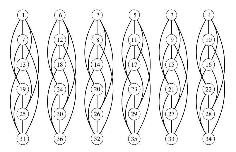
Figure 2. G-layers of an H (36, 8, 4).

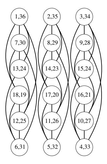
Figure 3. Edges of the Gamma graph induced by the G-layers.

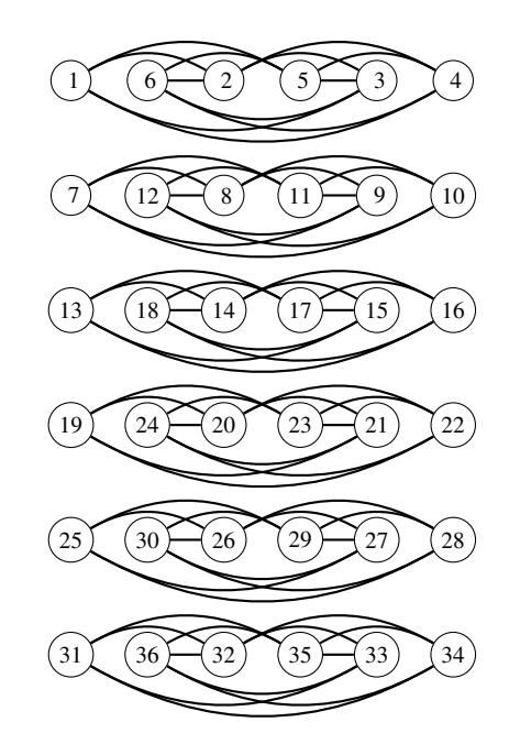
Figure 4. H-layers of an H (36, 8, 4).

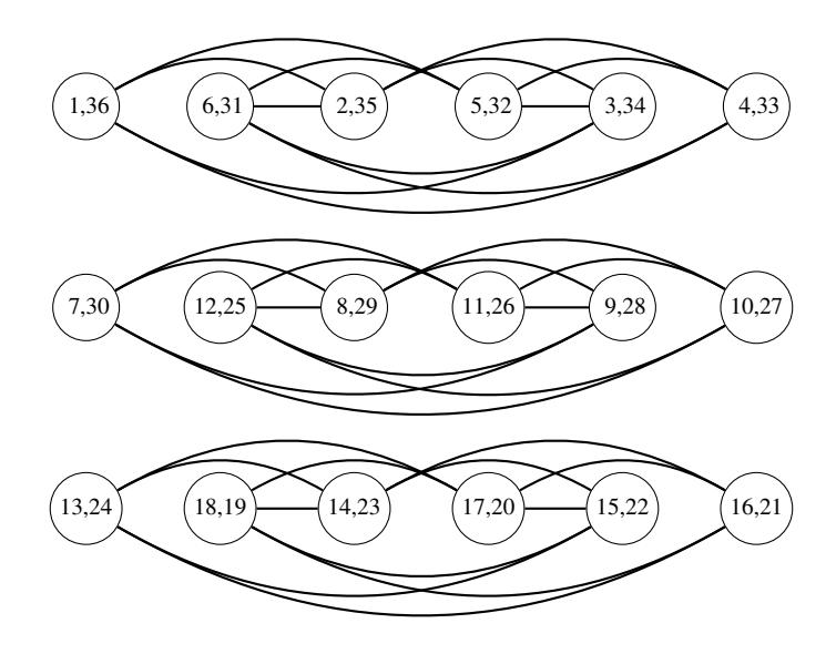
Figure 5. Edges of the Gamma graph induced by the H-layers.

5. New Results for Odd d

The construction in this section is a generalization of the class of 1-handicap graphs constructed by Froncek and Shepanik in [12] and [13]. As was the case for even d, our approach will be to first

construct a class of d-handicap graphs for a small regularity k, and then use the Gamma graph to add distance magic layers to increase k until the bound is met.

Theorem 5.1. For every odd positive integer d, there exists an H(n, 2d + 1, d) whenever

• \(n \equiv 0 \pmod{4d+4}\), \(n \ge (d+1)(d+3)\), and \(d \equiv 1 \pmod{4}\) or
• \(n \equiv 0 \pmod{4d+4}\), \(n \ge (d+1)(d+5)\), and \(d \equiv 3 \pmod{4}\) or
• \(n \equiv 2d + 2 \pmod{4d + 4}\), \(n \ge (d + 1)(d + 3)\), and \(d \equiv 3 \pmod{4}\).

Proof. Let \(G=K_{d+1}\) with vertex set \(V(G)=\{g_0,g_1,\ldots,g_d\}\). Define \(t=\frac{n}{d+1}\) and if \(d\equiv 1\ (\text{mod }4)\), let \(H=C_{\frac{t}{2}}\left(\frac{t}{4},1,2,\ldots,\frac{d-1}{4}\right)\circ\overline{K_2}\), otherwise let \(H=C_{\frac{t}{2}}\left(1,2,\ldots,\frac{d+1}{4}\right)\circ\overline{K_2}\). Let \(V(H)=\{h_0,h_1,\ldots,h_{t-1}\}\) where each pair of isolated vertices, \((h_j,h_{j+1})\) for \(j=0,2,\ldots,t-2\), corresponds to the blown-up vertices in H. Notice that if \(d\equiv 1\ (\text{mod }4)\), then \(n\geq (d+1)(d+3)\) implies \(\frac{d-1}{4}<\frac{t}{4}\). If \(d\equiv 3\ (\text{mod }4)\) and \(n\equiv 0\ (\text{mod }4d+4)\), then \(n\geq (d+1)(d+3)\) implies \(\frac{d+1}{4}<\frac{t}{4}\). Finally, if \(d\equiv 3\ (\text{mod }4)\) and \(n\equiv 2d+2\ (\text{mod }4d+4)\), then \(n\geq (d+1)(d+3)\) implies \(\frac{d+1}{4}\leq \frac{t-2}{4}\). Let \(\mathcal{G}=G\Box H\) and denote by \(x_i^j\) each vertex \((g_i,h_j)\in V(\mathcal{G})\) for all \(i=0,1,\ldots,d\) and \(j=0,1,\ldots,t-1\). Define \(l:V(\mathcal{G})\to\{1,2,\ldots,n\}\) by

\[l(x_i^j) = \begin{cases} ti + \frac{j+2}{2}, & j = 0, 2, \dots, t-2, \\ t(i+1) - \frac{j-1}{2}, & j = 1, 3, \dots, t-1. \end{cases}\]

for all i = 0, 1, ..., d. Clearly, l is a bijection.

Notice that \(l(x_i^j) + l(x_i^{j+1}) = t(2i+1) + 1\) for j = 0, 2, ..., t-2, so each pair \((l(x_i^j), l(x_i^{j+1}))\) is \(S_{i+1}\)-complements. For every vertex \(x_i^j \in V(\mathcal{G})\), we have

\[\begin{split} w(x_i^j) &= \sum_{p \neq i} l(x_p^j) + \frac{d+1}{2} [t(2i+1)+1] \\ &= \sum_{p=0,1,\dots,d} l(x_p^j) - l(x_i^j) + \frac{d+1}{2} [t(2i+1)+1] \\ &= \begin{cases} \frac{n(d+2i+1)+(d+1)(j+3)}{2} - l(x_i^j), \ j=0,2,\dots,t-2, \\ \frac{n(d+2i+3)-(d+1)(j-2)}{2} - l(x_i^j), \ j=1,3,\dots,t-1. \end{cases} \end{split}.\]

For every \(i = 0, 1, \dots, d\), define the sequences

\[s_i = l(x_i^0), l(x_i^2), \dots, l(x_i^{t-2}), l(x_i^{t-1}), l(x_i^{t-3}), \dots, l(x_i^3), l(x_i^1)\]

and

\[w_i = w(x_i^0), w(x_i^2), \dots, w(x_i^{t-2}), w(x_i^{t-1}), w(x_i^{t-3}), \dots, w(x_i^3), w(x_i^1).\]

Observe that \(l(x_i^{j+2}) - l(x_i^j) = 1\) for \(j = 0, 2, \dots, t-4, l(x_i^j) - l(x_i^{j+2}) = 1\) for \(j = 1, 3, \dots, t-3\), and \(l(x_i^{t-1}) - l(x_i^{t-2}) = 1\). Similarly, we have \(w(x_i^{j+2}) - w(x_i^j) = d\) for \(j = 0, 2, \dots, t-4\), \(w(x_i^j) - w(x_i^{j+2}) = d\) for \(j = 1, 3, \dots, t-3\), and \(w(x_i^{t-1}) - w(x_i^{t-2}) = d\). Therefore, \(s_i = ti + 1, ti + 2, \dots, ti + t\) and \(w_i = w(x_i^0), d + w(x_i^0), 2d + w(x_i^0), \dots, (t-1)d + w(x_i^0)\). Then since \(l(x_{i+1}^j) = l(x_i^j) + t\) and \(w(x_{i+1}^j) = w(x_i^j) + td\), for all \(i = 0, 2, \dots, d-1, j = 0, 1, \dots, t-1\), we conclude that the sequence \(s_0, s_1, \dots, s_d = 1, 2, 3, \dots, n\) and the sequence \(w_0, w_1, \dots, w_d = w_0, d + w_0, 2d + w_0, \dots, (n-1)d + w_0\), proving that \(\mathcal{G}\) is a d-handicap graph. Since \(\mathcal{G}\) is 2d + 1-regular, we have constructed an H(n, 2d + 1, d).

We will now employ the Gamma graph to give a wide range of possible densities given n and d.

Theorem 5.2. For every odd d, there exists an H(n, k, d) for every odd k such that \(2d + 1 \le k \le n - (2d + 3)\) whenever

• \(n \equiv 0 \pmod{4d+4}\), n > (d+1)(d+3), and \(d \equiv 1 \pmod{4}\) or
• \(n \equiv 0 \pmod{4d+4}\), \(n \ge (d+1)(d+5)\), and \(d \equiv 3 \pmod{4}\) or
• \(n \equiv 2d + 2 \pmod{4d + 4}\), \(n \ge (d + 1)(d + 3)\), and \(d \equiv 3 \pmod{4}\).

Proof. Let \(\mathcal{G}=G\square H\) be the \(H\left(n,2d+1,d\right)\) produced in Theorem 5.1 with d-handicap labeling l and recall that \(t=\frac{n}{d+1}\). Observe that \(l(x_i^j)+l(x_{d-i}^{j+1})=l(x_{d-i}^j)+l(x_i^{j+1})=n+1\) for \(i=0,1,\ldots,\frac{d-1}{2}\) and \(j=0,2,\ldots,t-2\). So the pairs \(\left(l(x_i^j),l(x_{d-i}^{j+1})\right),\left(l(x_{d-i}^j),l(x_i^{j+1})\right)\) partition \(\{1,2,\ldots,n\}\) into complements. Consider now \(\Gamma\left(\mathcal{G}\right)\). For \(i=0,1,\ldots,\frac{d-1}{2},\ j=0,2,\ldots,t-2\), we see that

\[V(\Gamma(\mathcal{G})) = \left\{ u_i^j = (x_i^j, x_{d-i}^{j+1}), u_i^{j+1} = (x_i^{j+1}, x_{d-i}^j) \right\}.\]

From here, the proof is essentially the same as the proof of Theorem 4.4 since the graphs G and H in this proof enjoy the same 1-factorability and symmetry properties as the graphs G and H from Theorem 4.4. Therefore, we omit the details.

Observe that if d=2c+1 for some nonnegative integer c, then we have constructed a k-regular d-handicap graph for every feasible regularity except the c smallest and the c largest possible regularities for any number of vertices n satisfying the hypothesis of the theorem. For example, if d=3, Theorem 5.2 provides a graph of every feasible regularity other than the single most sparse and single most dense graphs when \(n\equiv 0\pmod 8\). Combined with Theorem 3.6, we obtain the following corollary for 3-handicap regular graphs.

Corollary 5.1. If \(n \equiv 0 \pmod{8}\) and \(n \geq 24\), then there exists an H(n, k, 3) if and only if k is odd and \(5 \leq k \leq n-7\), except possibly when \(n \equiv 8, 16\), or \(24 \pmod{32}\) and \(k \in \{5, n-7\}\).

6. Conclusion

We have constructed many classes of k-regular d-handicap tournaments for every \(d \geq 1\), addressing the spectrum question for all three parameters; number of teams, number of games, and handicap number. Also, it is an easy observation that the complement of a d-handicap graph is a distance antimagic graph in which the weights form an arithmetic progression with difference -1-d. Therefore, in combination with results on distance magic graphs ("d=0"), we have provided infinite classes of graphs which can be labeled \(f(x_i)=i\) with the first n natural numbers such that the induced weights \(w(x_1), w(x_2), \ldots, w(x_n)\) form a d-arithmetic progression for any integer d.

One direction forward is to find constructions for the extreme values of k missed by Theorem 5.2 for \(d \ge 3\) or Theorem 4.4 for \(d \ge 4\). We conjecture that d-handicap graphs can be found for these missing parameters, but it will take a new approach perhaps not considered here. Another direction forward is to find classes of d-handicap graphs for the missing classes of n, for example d = 2 and \(n \equiv 4 \pmod{8}\).

References

• [1] B. Alspach and H. Gavlas, Cycle decompositions of Kⁿ and Kⁿ − I, J. Comb. Theory Ser. B 81 (2001) 77–99.
• [2] M. Anderson and M. Lipman, The wreath product of graphs, Graphs and Applications, John Wiley & Sons, New York, 1985, pp. 23–39.
• [3] S. Arumugam, D. Froncek, and N. Kamatchi, Distance magic graphs a survey, J. Indones. Math. Soc., Special Edition (2011), 1–9.
• [4] S. Arumugam and N. Kamatchi, On (a, d)-distance antimagic graphs, Australas. J. Combin. 54 (2012), 279–287.
• [5] S. Cichacz and D. Froncek, Distance magic circulant graphs, Discete Math. 339 (2016), 84– 94.
• [6] B. Freyberg, d-Handicap graphs of even order, Bull. Inst. Combin. Appl. 83 (2018), 102 111.
• [7] D. Froncek, Fair incomplete tournaments with odd number of teams and large number of games, Congr. Numer. 187 (2007), 83–89.
• [8] D. Froncek, Full spectrum of regular incomplete 2-handicap tournaments of order n ≡ 0 (mod 16), J. Combin. Math. Combin. Comput. 106 (2018), 175–184.
• [9] D. Froncek, A note on incomplete handicap tournaments with handicap two of order n ≡ 8 (mod 16), Opuscula Math. 37 (2017), 557–566.
• [10] D. Froncek, Regular handicap graphs of odd order, J. Combin. Math. Combin. Comput. 102 (2017), 253–266.
• [11] D. Froncek, P. Kovar, and T. Kovarova, Fair incomplete tournaments, Bull. Inst. Combin. Appl. 48 (2006), 31–33.
• [12] D. Froncek, A. Shepanik, On regular handicap graphs of order n ≡ 0 (mod 8), Electron. J. Graph Theory Appl. 6 (2) (2018), 208–218.
• [13] D. Froncek, A. Shepanik, Regular handicap graphs of order n ≡ 4 (mod 8), Electron. J. Graph Theory Appl. 10 (1) (2022), 259–273.
• [14] D. Froncek, A. Shepanik, P. Kovar, M. Kravcenko, A. Silber, T. Kovarova, B. Krajc, On regular handicap graphs of even order, Elect. Notes in Disc. Math., 60 (2017), 69–76.
• [15] V. Vilfred, On P−labelled Graphs and Circulant Graphs, Ph.D Thesis, University of Kerala, Trivandrum India, (1994).