Dominique Des´ erable ´
National Institute of Applied Sciences, Rennes, France
domidese@gmail.com
Arrowhead and diamond form a family of two hierarchical Cayley graphs defined on the triangular grid. In their undirected version, they are isomorphic and merely define two distinct representations of the same graph. This paper gives the expression of their diameter, in the oriented and non– oriented case. It also displays the full distribution of antipodals. This family could appear as a promising topology for Network–on–Chip architectures.
Keywords: Cayley graphs, interconnection networks, NoC, diameters, arrowhead & diamond
Mathematics Subject Classification : 05C12, 05C60, 68M10
DOI: 10.5614/ejgta.2025.13.1.6
1. Introduction
Networks are represented by graphs or digraphs: a vertex in the graph stands for a node in the network while an edge (resp. an arc) stands for a full–duplex (resp. half–duplex) communication link. The paper is concerned with a family of tori (i.e. arrowhead and diamond) which was defined on the triangular (or "hexavalent") grid [1]. Their related interconnection networks have several important advantages. They have a bounded degree and the highest allowed degree for a two–dimensional regular grid. They are good hosts for embedding the normal grid. As hierarchical Cayley graphs, they allow recursive constructions and divide–and–conquer schemes for information dissemination like broadcasting and gossiping [2–4]. They could accordingly provide a promising topology for Network–on–Chip "NoC" architectures, once the "diagonal" link be suitable for on–die implementation [5–7].
Received: 25 February 2020, Revised: 11 December 2024, Accepted: 8 March 2025.
In general, the topologies related to plane tessellations belong to the family of multi–loop – or circulant – networks [8]. The usual trend for two–dimensional hexavalent networks is a hexagonal torus HD with D circular rings of length 6D arranged around a central node, the order of HD is the centered hexagonal1 number ND = 3D2 + 3D + 1 and D is the diameter of HD. Incidentally, this family of "honeycombs" HD was encountered elsewhere, arising in various projects such as FAIM–1 [9], Mayfly [10] and HARTS [11]. It was the era of microcomputers, the era of networks of microcomputers organized into clusters and the era of the famous Cosmic Cube [12]. Eventually, this HD family emerged more recently with the "EJ" (as Eiseinstein–Jacobi) [13] networks [14].
On the wrong side, those circulant tilings are not easily scalable, as their respective OEIS sequence can attest. Indeed, they are Cayley graphs (i.e. graphs of groups) so they are regular but this property is not enough to fulfill our request for scalability. Scalability is a powerful feature for general–purpose computers and interconnection networks. This property allows divide–and– conquer strategies both for construction methods and for problem–solving methods. This is why another approach is addressed hereafter.
The topology of our arrowhead family [15] is quite different. The construction follows a recursive scheme and yields various representations of (directed) digraphs or (undirected) graphs, either as Sierpinski–like ´ arrowhead 2 or hexagonal hexarrowhead or either as lozenged diamond or square orthodiamond. The construction of arrowheads and diamonds, not isomorphic as digraphs, is induced by two possible orientations in the hexavalent lattice. In their undirected version, they are isomorphic and merely define two distinct representations of the same graph.
So far, the hexarrowhead underlies a cellular automata network used in the area of geomechanics as a framework to study the consistency of the model with the behavior of granular matter [17–19]. It was also applied to study its suitability for scale change in physical systems [20]. Besides, the orthodiamond, named "Tn" therein, is the subject of several works on cellular multiagent systems [21–24]: routing performances are compared with a subnetwork of Tn which is just the 2 n–ary 2–cube [25]. It is worth pointing out that another family of "augmented" k–ary 2–cubes was investigated elsewhere [26] for any k but which coincide with Tn only when k = 2n . As far as we are concerned and in order to preserve the morphism properties between arrowhead and diamond, that value k = 2n is mandatory.
Oriented and non–oriented diameters are important parameters that define the maximum distance from any vertex to another in digraphs and graphs and they provide lower bounds for routing and global communications. This paper is devoted to their study in the arrowhead family and yields their exact value as well as the full distribution of antipodals. In Sect. 2, we recall some general statement concerning Cayley graphs and arrowhead and diamond are redefined from [15]. Section 3 and Section 4 are devoted to the analysis of the distribution of the antipodals and the computation of the diameter, respectively for the undirected and the directed version of these graphs. A preliminary version of this paper has been published elsewhere [27].
1Sequence A003215 in the OEIS: 1, 7, 19, 37, 61, 91... — The On–Line Encyclopedia of Integer Sequences.
2We borrow the term "arrowhead" from Mandelbrot [16] about one of the Sierpinski's fractal constructions. ´
2. Arrowhead and Diamond
A Cayley graph or digraph \(\Gamma(\mathcal{G}, \mathcal{S})\) is constructed from a group \(\mathcal{G}\) and a generating set \(\mathcal{S} \in \mathcal{G}\). The vertex set is \(\mathcal{G}\) and the edge set \(\mathcal{G} \times \mathcal{S}\). Cayley graphs (the same remarks hold for digraphs) are regular of degree \(|\mathcal{S}|\). Their edge–connectivity \(\lambda\) (the minimum number of edges whose removal disconnects the graph) satisfies \(\lambda = |\mathcal{S}|\). They are vertex–transitive (or vertex–symmetric) in the sense that for any pair (u, u') of vertices there exists an automorphism of \(\Gamma\) that maps u into u'.
Definition 2.1. Given the group \(G_n = \mathbb{Z}_{2^n} \times \mathbb{Z}_{2^n}\) with \(n \in \mathbb{N}\):
- We define the directed arrowhead \(\overrightarrow{AT}_n = \Gamma(G_n, S^+)\) as the digraph of \(G_n\) with the generating set \(S^+ = (s_1, s_2, s_3) = ((-1, -1), (1, 0), (0, 1))\).
- Let \(S^- = (-s_1, -s_2, -s_3)\) be the set of inverses of \(S^+\) and let the generating set \(S = S^+ \cup S^-\) now closed under inverses. We define the undirected arrowhead as \(\mathcal{AT}_n = \Gamma(G_n, S)\).
- We define the directed diamond \(\overset{\rightarrow}{\mathcal{DT}}_n = \Gamma(G_n, T^+)\) as the digraph of \(G_n\) with the generating set \(T^+ = (t_1, t_2, t_3) = (-s_1, s_2, s_3) = ((1, 1), (1, 0), (0, 1))\).
- Let \(T^- = (-t_1, -t_2, -t_3)\) be the set of inverses of \(T^+\) and let the generating set \(T = T^+ \cup T^-\) now closed under inverses. We define the undirected diamond as \(\mathcal{DT}_n = \Gamma(G_n, T)\).
- \(\mathcal{DT}_n\) and \(\mathcal{AT}_n\) are isomorphic since T = S.
The order of these graphs is given by \(N = |G_n| = 4^n\) and the number of arcs (or edges) by \(\frac{1}{2}|S||G_n| = 3N\). In the sequel, the detection of antipodals and the computation of diameters will follow an inductive scheme. It is therefore convenient to exploit the recursive structure of the graphs as follows.
Definition 2.2. Let \(0 \le k \le n\) and let again
\[G_n = \{(x, y) = xs_2 + ys_3 \mid x, y \in \mathbb{Z}_{2^n}\}\] (1)
be the vertex set expressed from the previous definition and let
\[G_{n,k} = \mathbf{2}^k \cdot G_{n-k} = \{ (2^k x, 2^k y) \mid x, y \in \mathbb{Z}_{2^{n-k}} \}\] (2)
be the subgroup of \(G_n\) generated by \(2^k S^+ = \{ 2^k s \mid s \in S^+ \}.\)
We define \(\mathcal{AT}_{n,k} = \Gamma(G_{n,k}, \mathbf{2}^k S^+)\) isomorphic to \(\mathcal{AT}_{n-k}\) as the digraph of \(G_{n,k}\) with the generating set \(\mathbf{2}^k S^+\).
As a matter of fact, this statement gives an embedding scheme of \(\overrightarrow{\mathcal{AT}}_{n-k}\) into \(\overrightarrow{\mathcal{AT}}_n\) with dilation \(2^k\). A definition of digraph \(\overrightarrow{\mathcal{DT}}_{n,k}\) and of their undirected counterpart will follow from a similar statement.
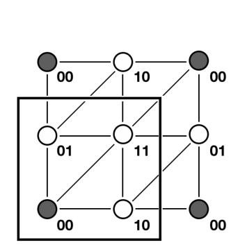
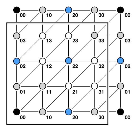
Figure 1. Representation of T1 and T2 – some vertices are replicated for convenience.
In the following, the undirected –isomorphic– graphs AT n and DT n will be denoted as Tn. The representation of T1 and T2 is displayed in Fig. 1.
T0 is not displayed, reduced to the single vertex of G0 = {(0, 0)} as a 6–valent vertex. It should be observed in (2) that Gn,0 = Gn and Gn,n = G0.
In T1 we observe that G1,0 = G1 = {(0, 0),(1, 1),(1, 0),(0, 1)} with 4 vertices and that G1,1 = 2· G0 = {(0, 0)}.
In T2 one get G2 = {( x, y ) = xs2 + ys3 | x, y ∈ Z4} with 16 vertices and see that G2,1 = 2· G1 = {(0, 0),(2, 2),(2, 0),(0, 2)} isomorphic to G1 and that G2,2 = 4· G0 = {(0, 0)}.
3. Non–Oriented Diameter
The diameter of a graph is the maximum distance between any pair of vertices. We call "oriented" (resp. "non–oriented") the diameter of a directed (resp. undirected) graph. Two vertices are said to be antipodal if their distance is the diameter. Without loss of generality, we can compute the diameter as the length of the shortest path from the "origin" (0, 0) to an antipodal since the graphs are vertex–transitive. Hereafter, the term "antipodal" will be viewed from that vertex.
3.1. Diameter in Tn
In Fig. 1, it appears as trivial that vertices in subset {(1, 1),(1, 0),(0, 1)} in T1 are antipodal and at distance 1. We claim that in T2 the subset {(1, 2),(1, 3),(2, 3)} as well as its symmetric part {(2, 1),(3, 1),(3, 2)} are antipodal at distance 2. To sketch the proof, let us fix x ≤ y and then extend to the triangular diagrams in Fig. 2. Beforehand we give the following definitions.
Definition 3.1. Herein, for n > 0, the ordered subset Ωn will always denote an antipodal 3–cycle in Tn and Ωn,1 will denote the image of Ωn−1 whereas Ωn,2 will denote the image of Ωn−1,1 under the mapping induced by (2). Thus we have
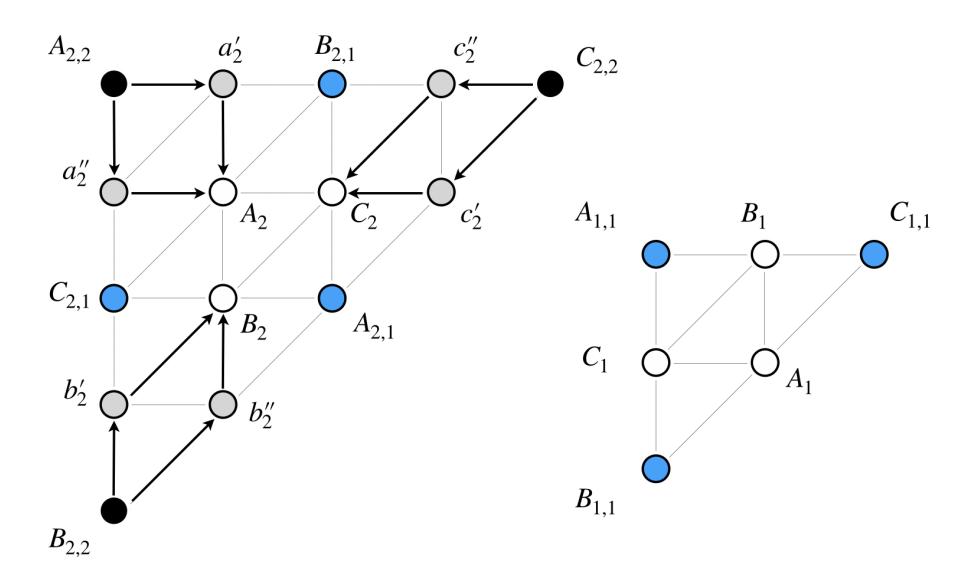
Figure 2. Triangular diagram of T2 and T1. Induction from T1 to T2. Resulting shortest paths to antipodals in T2.
- Ω0 = {(0, 0)}
- Ω1 = ((1, 1),(1, 0),(0, 1))
• \[\Omega_{n,1} = 2 \cdot \Omega_{n-1} = \{ (2x, 2y) \mid x, y \in \Omega_{n-1} \}\] \((n > 0)\)
• \[\Omega_{n,2} = 2 \cdot \Omega_{n-1,1} = \{ (2x, 2y) \mid x, y \in \Omega_{n-1,1} \} = 4 \cdot \Omega_{n-2}\] \((n > 1)\)
In the sequel, the term image will always mean the image under the isomorphic mapping in Def. 3.1. Note that any Ωn,k is a subset of Gn,k. In the diagrams of Fig. 2 and further, the vertices of those different subsets will be labeled as follows:
- Ωn = (An, Bn, Cn)
- Ωn,1 = (An,1, Bn,1, Cn,1)
- Ωn,2 = (An,2, Bn,2, Cn,2).
Lemma 3.1. Let Dn be the non–oriented diameter of Tn. Then D0 = 0 and Dn = 2Dn−1 + 1 or Dn = 2Dn−1 depending upon the odd–even parity of n.
Proof : We prove by induction and refer first to Fig. 2. For the base case n = 1 the vertices of Ω1,1 coincide as origin at distance 0 and vertex set Ω1 is trivially antipodal at distance D1 = 1. For n = 2, vertex set Ω2,2 as image of Ω1,1 coincide as origin at distance 0. Now, vertices (a ′ 2 , a′′ 2 ),(b ′ 2 , b′′ 2 ),(c ′ 2 , c′′ 2 ) reachable from (A2,2, B2,2, C2,2) are at distance 1 and then the triple (A2, B2, C2) is at distance 2. Besides, vertices of Ω2,1 as image of Ω1 are by induction at distance 2D1 = 2. Therefore the triple Ω2 is antipodal, as well as Ω2,1 and at distance the diameter D2 = 2.
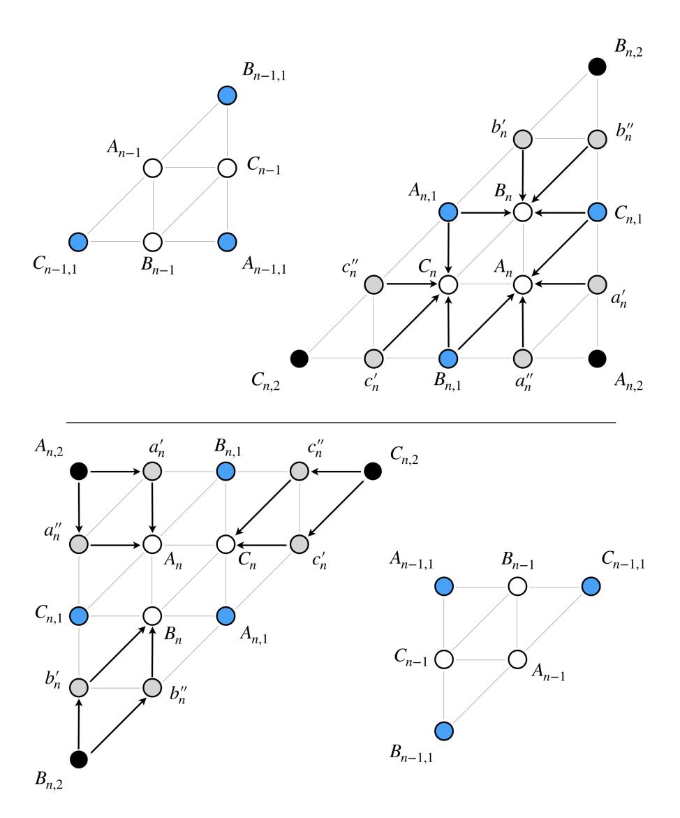
Figure 3. Triangular diagrams in Tn – for n odd (↑) – for n even (↓).
• n odd: Let Ωn,1 and Ωn,2 be the respective images of Ωn−1 and Ωn−1,1 in upper Fig. 3. From induction, vertices of those both triples are assumed at distance 2Dn−1. Now the six vertices (a ′ n , a′′ n ),(b ′ n , b′′ n ),(c ′ n , c′′ n ) are also at distance 2Dn−1 : a ′ n and An,2 are reachable from a common antecedent
\[(x_{a'_n}, y_{a'_n}) + t_2 = (x_{A_{n,2}}, y_{A_{n,2}}) + t_1\]
and idem for a ′ n and Cn,1
\[(x_{a'_n}, y_{a'_n}) + t_1 = (x_{C_{n,1}}, y_{C_{n,1}}) + t_2\]
and so forth.Therefore those six vertices are at distance 2Dn−1. Vertex An can then be reached through (a ′ n , a′′ n ), Bn through (b ′ n , b′′ n ), Cn through (c ′ n , c′′ n ). The triple (An, Bn, Cn) can also be reached from
\[(B_{n,1}, C_{n,1}), (C_{n,1}, A_{n,1}), (A_{n,1}, B_{n,1}).\]
It is therefore antipodal, at distance the diameter Dn = 2Dn−1 + 1.
• n even: Let Ωn,2 be the image of Ωn−1,1 in lower Fig. 3 and, from induction, with vertices assumed at distance 2(Dn−1 − 1). The three pairs (a ′ n , a′′ n ),(b ′ n , b′′ n ),(c ′ n , c′′ n ) reachable from (An,2, Bn,2, Cn,2) are at distance 2(Dn−1 − 1) + 1 = 2Dn−1 − 1. Vertex An can be reached through (a ′ n , a′′ n ), Bn through (b ′ n , b′′ n ), Cn through (c ′ n , c′′ n ) and then the triple (An, Bn, Cn) is at distance (2Dn−1 −1) + 1 = 2Dn−1. Besides, Ωn,1 as image of Ωn−1 has also its vertices at distance 2Dn−1. Therefore the triple (An, Bn, Cn) is antipodal, as well as (An,1, Bn,1, Cn,1) and at distance the diameter Dn = 2Dn−1. ✷
Lemma 3.2. Two useful relations are exhibited.
\[\forall n > 0: D_{n-1} + D_n = 2^n - 1 \tag{3}\]
\[\forall n > 1: D_n - D_{n-2} = 2^{n-1} \tag{4}\]
Proof : Let us rewrite Dn = 2Dn−1 + εn from Lemma 3.1 where εn ≡ n (mod 2). Given un = Dn−1 + Dn we note that u1 = 1 and show that un+1 = 2un + 1. Now un+1 = Dn + Dn+1 = (2Dn−1 + εn) + (2Dn + εn+1) but εn + εn+1 = 1 for any n whence un+1 = 2un + 1 and (3) results from an obvious induction.
For (4) we note from above that \[D_n - D_{n-2} = u_n - u_{n-1} = 2^{n-1}\].
Proposition 3.1. Tn has the diameter
\[D_n = \frac{2\sqrt{N} - 1}{3}\] or \(D_n = \frac{2(\sqrt{N} - 1)}{3}\)
depending on the odd–even parity of n.
Proof : Follows from Lemma 3.1. For n odd, Dn = 2Dn−1 + 1 and by (3) Dn−1 = (2n − 1) − Dn whence 3Dn = 2 · 2 n − 1. For n even, Dn = 2Dn−1 whence 3Dn = 2 · (2n − 1). ✷
The ten first values of Tn diameter are displayed below.
| n | 0 | 1 | 2 | 3 | 4 | 5 | 6 | 7 | 8 | 9 |
|---|---|---|---|---|---|---|---|---|---|---|
| N | 1 | 4 | 16 | 64 | 256 | 1024 | 4096 | 16384 | 65536 | 262144 |
| Dn | 0 | 1 | 2 | 5 | 10 | 21 | 42 | 85 | 170 | 341 |
3.2. Antipodals in Tn
Some relevant properties of antipodal coordinates are highlighted hereafter and antipodals are enumerated.
Proposition 3.2. The antipodal coordinates in Ωn satisfy:
- n odd: ( xCn , yCn ) = ( Dn−1, Dn )
- n even: ( xBn , yBn ) = ( Dn−1, Dn ).
Proof : This is true for n = 1 where ( xC1 , yC1 ) = (0, 1) = ( D0, D1 ) and for n = 2 where ( xB2 , yB2 ) = (1, 2) = ( D1, D2 ) referring back to Fig. 1 and Fig. 2.
- n odd (upper Fig. 4): assume ( xBn−1 , yBn−1 ) = ( Dn−2, Dn−1 ). Then ( xBn,1 , yBn,1 ) = ( 2Dn−2, 2Dn−1 ) = ( Dn−1, Dn − 1) since n − 1 is even when n is odd, whence ( xCn , yCn ) = ( xBn,1 , yBn,1 ) + (0, 1).
- n even (lower Fig. 4): assume ( xCn−1 , yCn−1 ) = ( Dn−2, Dn−1 ). Then ( xCn,1 , yCn,1 ) = ( 2Dn−2, 2Dn−1 ) = ( Dn−1 − 1, Dn) since n − 1 is odd when n is even, whence ( xBn , yBn ) = ( xCn,1 , yCn,1 ) + (1, 0). ✷
Coordinates of other antipodals are simply deduced.
Referring back to Fig. 1 we now focus on the subset {(2, 1),(3, 1),(3, 2)}, antipodal by symmetry. By fixing x ≥ y and as from Def. 3.1 we define the symmetric subsets
- Ωn = (An, Bn, Cn)
- Ωn,1 = (An,1, Bn,1, Cn,1)
- Ωn,2 = (An,2, Bn,2, Cn,2)
where ( xAn , yAn ) = ( −xAn , −yAn ) and where any vertex in those subsets is defined in that way.
Proposition 3.3. The antipodal coordinates in Ωn satisfy:
- n odd: ( xBn , yBn ) = ( Dn, Dn−1 )
- n even: ( xCn , yCn ) = ( Dn, Dn−1 ).
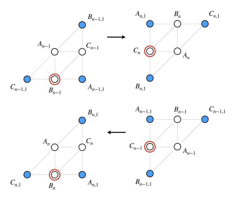
Figure 4. Antipodal coordinates in Tn – for n odd (↑) – for n even (↓).
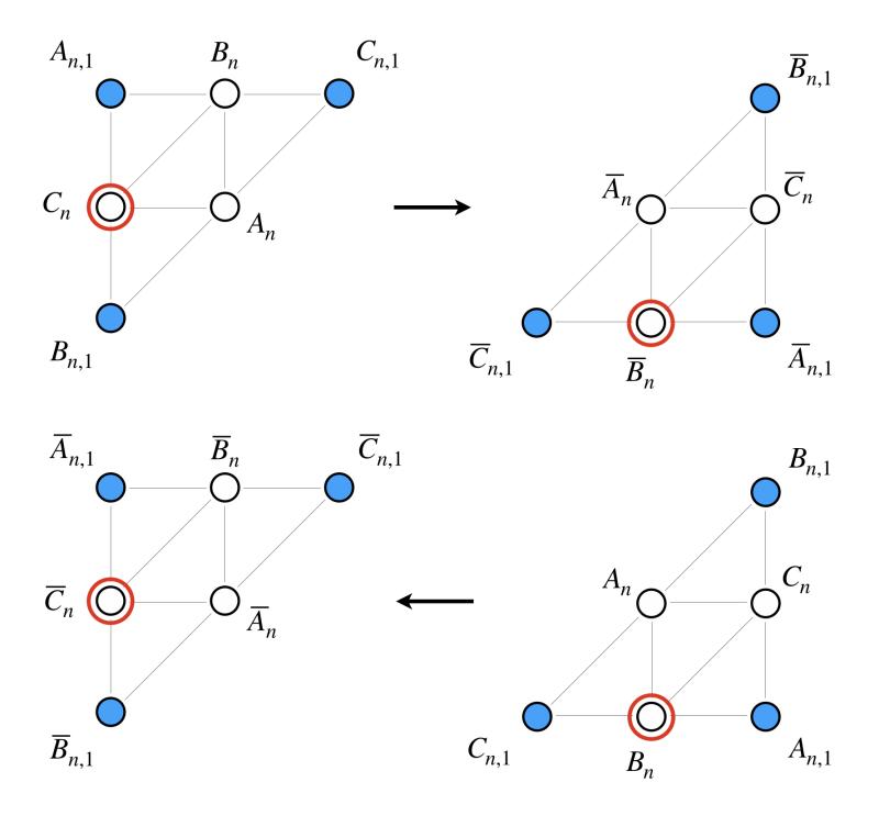
Figure 5. Antipodal inverses in Tn – for n odd (↑) – for n even (↓).
Proof: From Proposition 3.2 and Fig. 5.
• n odd: \((x_{B_n}, y_{B_n}) = (x_{C_n}, y_{C_n}) + (1, 1)\) whence
\[(x_{\overline{B}_n}, y_{\overline{B}_n}) = (-D_{n-1} - 1, -D_n - 1)\]
and (3) yields \((x_{\overline{B}_n}, y_{\overline{B}_n}) = (D_n, D_{n-1})\) by a simple reduction in \(\mathbb{Z}_{2^n}\).
• \(n \text{ even: } (x_{C_n}, y_{C_n}) = (x_{B_n}, y_{B_n}) + (1, 1) \text{ whence}\)
\[(x_{\overline{C}_n}, y_{\overline{C}_n}) = (-D_{n-1} - 1, -D_n - 1)\]
whence again the result.
Corollary 3.1. The antipodal inverses satisfy for any n:
- \(\bullet (x_{\overline{A}_n}, y_{\overline{A}_n}) = (y_{A_n}, x_{A_n})\)
- \(\bullet (x_{\overline{B}_n}, y_{\overline{B}_n}) = (y_{C_n}, x_{C_n})\)
\[\bullet (x_{\overline{C}_n}, y_{\overline{C}_n}) = (y_{B_n}, x_{B_n})\]
Coordinates of other antipodals subsets are simply deduced.
Corollary 3.2. Let \(\mathcal{N}_{A,n}\) be the number of antipodals in \(\mathcal{T}_n\). Then
- \(\mathcal{N}_{A_1} = |\Omega_1 \cup \overline{\Omega}_1| = |\Omega_1| = 3\)
- \(\mathcal{N}_{\mathcal{A},2} = |\Omega_2 \cup \overline{\Omega}_2| + |\Omega_{2,1} \cup \overline{\Omega}_{2,1}| = |\Omega_2 \cup \overline{\Omega}_2| + |\Omega_{2,1}| = 9\)
• \[\text{[rumus tidak dapat ditampilkan dengan baik — lihat PDF asli]}\]
depending on the odd–even parity of n > 2.
We observe that \(\Omega_1\) and \(\overline{\Omega}_1\) coincide and that \(\Omega_{2,1}\) and \(\overline{\Omega}_{2,1}\) coincide.
4. Oriented Diameter
4.1. Diameter and Antipodals in \(\overrightarrow{AT}_n\)
We now refer to digraph \(\overrightarrow{\mathcal{AT}}_n\) in Def. 2.1 with its generating set \(S^+\) highlighted in the inset of Fig. 6. Again it appears as trivial that vertices in subset \(\{(1,1),(1,0),(0,1)\}\) in \(\overrightarrow{\mathcal{AT}}_1\) are antipodal and at distance 1 from the origin (0,0). We claim that in \(\overrightarrow{\mathcal{AT}}_2\) the subset \(\{(1,2),(1,3),(2,3)\}\) as well as its symmetric part \(\{(2,1),(3,1),(3,2)\}\) are antipodal at distance 3. To sketch the proof, let us again fix \(x \leq y\) and then extend to the triangular diagrams in Fig. 7.
Lemma 4.1. Let \(\vec{D}_n\) be the oriented diameter of \(\vec{\mathcal{AT}}_n\). Then \(\vec{D}_0 = 0\) and \(\vec{D}_n = 2\vec{D}_{n-1} + 1\) for n > 0.
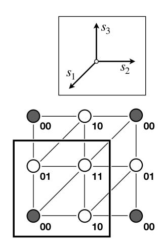
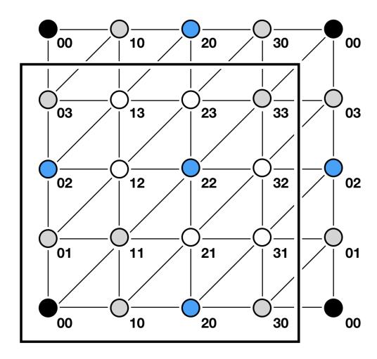
Figure 6. Orientation in \(\overrightarrow{\mathcal{AT}}_1\) and \(\overrightarrow{\mathcal{AT}}_2\) – orientation highlighted in the inset.
Proof: \(\vec{D}_0 = 0\) and in \(\vec{\mathcal{AT}}_1\) the triple \((A_1, B_1, C_1) = ((1, 1), (1, 0), (0, 1))\) is clearly antipodal and \(\vec{D}_1 = 1\). Let \(A_{n,2}\) be the image of \(A_{n-1,1}\) whatever the parity of n, and assumed from induction at distance \(2(\vec{D}_{n-1} - 1)\). There exists a directed path
\[(A_{n,2} \to a'_n \to a''_n \to A_n)\]
of length 3 from \(A_{n,2}\) to \(A_n\) therefore \(A_n\) is at distance \(2(\vec{D}_{n-1}-1)+3=2\vec{D}_{n-1}+1\). Idem for \((B_{n,2}\to B_n)\) and \((C_{n,2}\to C_n)\).
Besides the triple \((A_{n,1}, B_{n,1}, C_{n,1})\) as image of \((A_{n-1}, B_{n-1}, C_{n-1})\) is at distance \(2\vec{D}_{n-1}\) by induction. The triple \((A_n, B_n, C_n)\) is then also reachable either from \((C_{n,1}, A_{n,1}, B_{n,1})\) for n odd or from \((B_{n,1}, C_{n,1}, A_{n,1})\) for n even. It is therefore antipodal and at distance the diameter \(\vec{D}_n = 2\vec{D}_{n-1} + 1\).
Proposition 4.1. \(\overrightarrow{AT}_n\) has the diameter \(\overrightarrow{D}_n = \sqrt{N} - 1\) and the number of antipodals
• \(\mathcal{N}_{\vec{\mathcal{A}},1} = |\Omega_1 \cup \overline{\Omega}_1| = |\Omega_1| = 3\)
• \[\mathcal{N}_{\vec{\mathcal{A}},n} = |\Omega_n \cup \overline{\Omega}_n| = 6\] \((n > 1)\)
4.2. Diameter and Antipodals in \(\overrightarrow{\mathcal{DT}}_n\)
We now refer to digraph \(\overrightarrow{\mathcal{DT}}_n\) with its generating set \(T^+ = (t_1, t_2, t_3) = ((1, 1), (1, 0), (0, 1))\) in Def. 2.1.
Proposition 4.2. \(\overrightarrow{DT}_n\) has the diameter \(\overrightarrow{D}_n = \sqrt{N} - 1\) and the number of antipodals
• \(\mathcal{N}_{\vec{\mathcal{D}},n} = 2\sqrt{N} - 1\) for any \(n \in \mathbb{N}\).
Proof: The proof here is rather trivial: there is 1 vertex at distance 0, there are 3 vertices at distance 1, there are 2p+1 vertices at distance p and therefore \(2(2^n-1)+1=2^{n+1}-1\) vertices at distance \(2^n-1\).
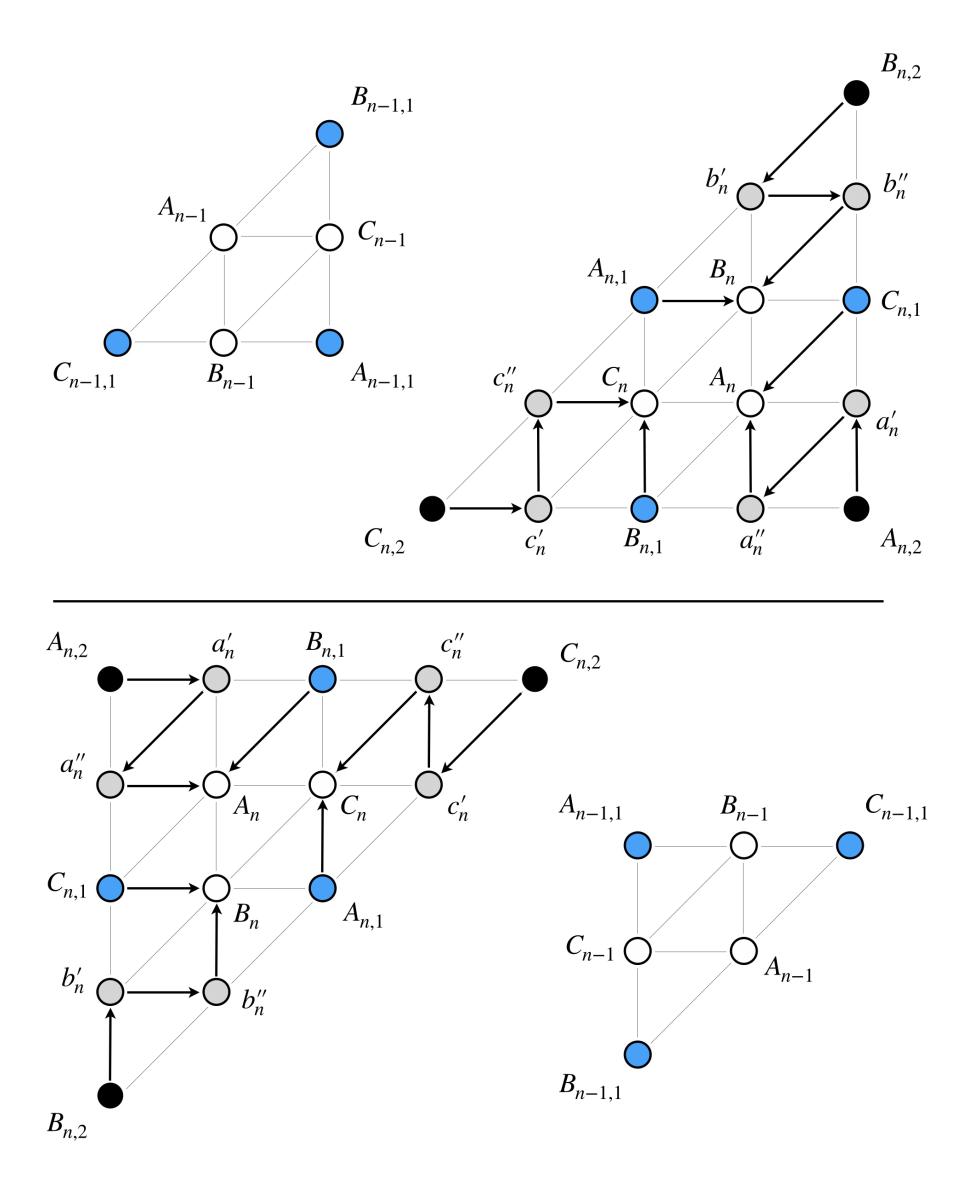
Figure 7. Triangular diagrams in \(\stackrel{\rightarrow}{\mathcal{AT}}_n\) – for n odd \((\uparrow)\) – for n even \((\downarrow)\).
5. Conclusion
Arrowhead and diamond form a family of two hierarchical Cayley graphs defined on the triangular grid. In their undirected version, they are isomorphic and merely define two distinct representations of the same graph. This paper gives the exact expression of their diameter, in the oriented and non– oriented case as well as the full distribution of antipodals.
This family of Cayley graphs could appear as a promising topology for Network–on–Chip "NoC" architectures. To our knowledge, we have no trace of this topology in the field of NoC and this lack would open an immense challenge. A possible hindrance could be the fulfillment of wires at angles other than the common angles (0, π/2) – namely either π/4 for the orthodiamond or kπ/3 for the hexarrowhead, even if some achievements seem to deny this intricacy [28, 29]. Prototyping simulations will be planned in the near future.
Acknowledgement
I am very grateful towards a reviewer of an ancient version of this article and who suggested a complete redefinition of the graphs presented a first time in [1], a redefinition which greatly supported the elaboration of this article.
References
- [1] D. Des´ erable, A family of Cayley graphs on the hexavalent grid, ´ Discrete Applied Math. 93(2-3) (1999) 221–241
- [2] D. Des´ erable, Broadcasting in the arrowhead torus, ´ Computers and Artificial Intelligence 16(6) (1997) 545–559
- [3] M.C. Heydemann, N. Marlin, S. Perennes, Complete rotations in Cayley graphs, ´ European J. Combinatorics 22(2) (2001) 179–196
- [4] D. Des´ erable, Systolic dissemination in the arrowhead family, ACRI 2014, J. Wa¸s, G. Sirak- ´ oulis, S. Bandini, eds., LNCS 8751 (2014) 75–86
- [5] D.N. Jayasimha, B. Zafar, Y. Hoskote, On–Chip Interconnection Networks: why they are different and how to compare them, Intel Corporation (2006) 1–11
- [6] D.B. Balfour, W.J. Dally, Design tradeoffs for tiled CMP on–chip networks, ICS 2006 Int. Conf. Supercomp. (2006) 187–198
- [7] E. Salminen, A. Kulmala, T.D. Ham¨ al¨ ainen, On network–on–chip comparison, DSD 2007 ¨ Digital System Design: Architectures, Methods and Tools (2007) 503–510
- [8] J.C. Bermond, F. Comellas, D.F. Hsu, Distributed loop computer networks: a survey, J. Par. Dist. Comp. 24 (1995) 2–10
- [9] A.L. Davis, S.V. Robison, The architecture of the FAIM-1 symbolic multiprocessing system, Proc. 9th Int. Joint. Conf. on Artificial Intelligence (1985) 32–38
- [10] A. Davis, Mayfly a general-purpose, scalable, parallel processing architecture, J. LISP and Symbolic Computation 5 (1992) 7–47
- [11] M.S. Chen, K.G. Shin, and D.D. Kandlur, Addressing, routing and broadcasting in hexagonal mesh multiprocessors, IEEE Trans. Comp. 39 (1) (1990) 10–18
- [12] C.L. Seitz, The Cosmic Cube, Comm. ACM 28(1) (1985) 22–33
- [13] K.P. Huber, Codes over Eisenstein–Jacobi integers, Finite Fields: Theory, Applications & Algorithms, G.L. Mullen, P.J.S. Shiue, eds., Contemporary Math. 168 (1994) 165–179
- [14] B. Albader, B. Bose, and M. Flahive, Efficient communication algorithms in hexagonal mesh interconnection networks, IEEE Trans. Par. Dist. Sys. 23 (1) (2012) 69–77
- [15] D. Des´ erable, Versatile topology for two–dimensional cellular automata, ´ Advances in Cellular Automata, A. Adamatzky, G.Ch. Sirakoulis, G.J. Mart´ınez (eds), Emergence, Complexity and Computation 52 (2025), 151–186.
- [16] B.B. Mandelbrot, The fractal geometry of nature, Freeman and Cie (1982)
- [17] D. Des´ erable, A versatile two-dimensional cellular automata network for granular flow, ´ SIAM J. Applied Math. 62 (4) (2002) 1414–1436
- [18] D. Des´ erable, S. Masson, and J. Martinez, Influence of exclusion rules on flow patterns in a ´ lattice-grain model, Powders & Grains, Kishino, Y. (ed.) Balkema (2001) 421–424
- [19] D. Des´ erable, Propagative mode in a lattice-grain CA: time evolution and timestep synchro- ´ nization, ACRI 2012 – G. Sirakoulis, S. Bandini, eds., LNCS 7495 (2012) 20–31
- [20] D. Des´ erable, Embedding Kadanoff's scaling picture into the triangular lattice, ´ Acta Phys. Pol. B Proc. Suppl. 4 (2) (2011) 249–265
- [21] P. Ediger, R. Hoffmann, and D. Des´ erable, Routing in the triangular grid with evolved agents, ´ J. Cellular Automata 7(1) (2012) 47–65
- [22] P. Ediger, R. Hoffmann, and D. Des´ erable, Rectangular ´ vs. triangular routing with evolved agents, J. Cellular Automata 8(1–2) (2013) 73–89
- [23] R. Hoffmann, D. Des´ erable, All-to-All communication with cellular automata agents in 2 ´ d Grids – Topologies, streets and performances, J. Supercomp. 69 (1) (2014) 70–80
- [24] R. Hoffmann and D. Des´ erable, Routing by cellular automata agents in the triangular lattice, ´ Robots and Lattice Automata, G.Ch. Sirakoulis, A. Adamatzky (eds), Emergence, Complexity and Computation 13 (2015) 117–147
- [25] W.J. Dally and C.L. Seitz, The torus routing chip, Distributed Computing 1 (1986) 187–196
- [26] Y. Xiang and I.A. Stewart, Augmented k–ary n–cubes, Information Sci. 181 (1) (2011) 239– 256
- [27] D. Des´ erable, Arrowhead and diamond diameters, arXiv.org/abs/2205.00489 (2022) 1–17 ´
- [28] W.-H. Hu, Eun Lee,and N. Bagherzadeh, Dmesh: a diagonally-linked mesh Network-on-Chip architecture, api.semanticscholar.org/CorpusID:17633766
- [29] M.H. Furhad and J.-M. Kim, An extended diagonal mesh topology for Network-on-Chip architectures, Int. J. Multimedia and Ubiquitous Eng. 10 (10) (2015) 197–210