Andrea Rey
Laboratorio de Investigacion y Desarrollo Experimental en Computaci ´ on (LIDEC), ´ Secretary of Research, Universidad Nacional de Hurlingham (UNAHUR), Buenos Aires, Argentina
Centro de Procesamiento de Senales e Im ˜ agenes (CPSI), ´ Facultad Regional Buenos Aires, Universidad Tecnologica Nacional (UTN), ´ Buenos Aires, Argentina
andrea.rey@unahur.edu.ar
It is well-known that Pareto distribution and related generalizations have historically been considered suitable for modeling income and wealth distributions, among other fields. Nowadays, graphs can be used to model many types of relations and processes in physical, biological, social, and information systems. By combining both concepts, this paper introduces the notion of the Pareto graph and gives some sufficient conditions to determine the existence of a giant component. A simulation study is carried out to evaluate the performance of Pareto random graph generation. In addition, basic graph properties of this novel kind of graph are contrasted with well-known models for random graph generation. The results are applied to real-life data that come from social networks, under the assumption that the degree distribution is well fitted by a Generalized Pareto distribution and compared with the fitting by other heavy-tailed distributions.
Keywords:
generalized Pareto distribution, random graphs, giant component, social networks
Mathematics Subject Classification : 05C80, 94C15
DOI: 10.5614/ejgta.2025.13.1.7
Received: 11 September 2020, Revised: 8 March 2025, Accepted: 21 March 2025.
1. Introduction
Large amounts of data can be visually represented using graphs, allowing an easier understanding of patterns, possible trends, and relations. The graph model is a powerful tool for knowing hidden information in raw data. Hence, graphs provide structures that can help make decisions.
A graph is a mathematical object widely employed in natural sciences, technological and business environments, and other knowledge areas. Graph Theory arose with the famous Konisberg's bridges problem formulated by Euler in the XVIII century. Although abundant computer programs for graph generation are available nowadays, users should deal with some basic definitions and principles. In this section, some of these elementary concepts are introduced.
1.1. Graphs and random graphs
A graph G consists of a non-empty finite set V (G) of vertices together with a finite set E(G) (possibly empty) of edges such that:
- each edge joins two distinct vertices in V (G), and
- any two distinct vertices in V (G) are joined by at most one edge, in other words, either they are not joined by an edge or joined by exactly one edge.
The theory of random graphs was founded by Erdos and R ˝ enyi [6, 7, 8]. In a simple manner, ´ we can think of a random graph as a living organism that evolves with time, which is born as a set of n isolated vertices and develops by successively acquiring edges at random. It is interesting to determine at what stage of the evolution a particular property of the graph is likely to arise.
Another established random graph model was proposed by Barabasi and Albert [1]. They ´ observe the continuous expansion of large networks by the addition of new vertices that show a proclivity to be attached to well-connected sites. Thus, their proposal is based on the feature that the connections between vertices in many large networks follow a scale-free power-law distribution. This means that a vertex in the network interacts with k other vertices with probability P(k) ∼ k −ω , where ω > 0 is named the power.
An automorphism of a graph is a permutation of the vertex set that preserves connections between two vertices. In [3], the authors show that a typical random graph is similar to an ideal regular graph, i.e. all the vertices have the same degree, whose automorphism group is transitive on small sets of vertices. There is no such non-trivial regular graph, and in many applications, random graphs are used precisely because they approximate an ideal regular graph.
The degree of a vertex is defined as the number of edges adjacent to this vertex. Let G be an undirected graph with vertices V = {1, 2, . . . , n} and let d1, d2, . . . , dn be the respective degrees of these vertices. The vector d = (d1, d2, . . . , dn) is usually called the degree sequence of G. Considering the degree sequence as a random variable, it makes sense to study the corresponding degree distribution.
Following the ideas developed in [15], if pk is the probability that a randomly chosen vertex in the graph has degree k, i.e. the proportion among the total of vertices that have degree k, we consider the generating function for the probability distribution of vertex degrees given by
\[G_0(x) = \sum_{k=0}^{+\infty} p_k x^k.\] (1)
Since the probability distribution is normalized and positive definite, \(G_0(x)\) is also absolutely convergent for all \(|x| \leq 1\), and hence it has no singularities in this region. Moreover, the distribution of outgoing edges is generated by the following function
\[G_1(x) = \frac{G_0'(x)}{G_0'(1)}. (2)\]
1.2. Pareto distribution
In [16], Pareto introduced the concept of Pareto distribution observing that in many populations, the number of individuals whose income exceeded a given level x was well approximated by \(Cx^{-\alpha}\) for some real number C and some \(\alpha > 0\). Several years later, Pickands introduced what he called a Generalized Pareto distribution in the context of the study of peaks over thresholds [17].
Throughout this paper, we use the Generalized Pareto Type II (GPDII) distribution given by its probability density function (pdf) defined as
\[f_P(x) = \frac{\alpha}{\sigma} \left( 1 + \frac{x - \mu}{\sigma} \right)^{-\alpha - 1},\tag{3}\]
and its cumulative distribution function (cdf) is defined as
\[F_P(x) = 1 - \left(1 + \frac{x - \mu}{\sigma}\right)^{-\alpha},\tag{4}\]
where \(\mu \in \mathbb{R}\), \(\alpha, \sigma > 0\) and the support is \(x \ge \mu\). Notice that if \(\mu = \sigma\) we obtain the form of the Generalized Pareto Type I pdf: \(f_P(x) = \alpha \sigma^{\alpha} x^{-\alpha-1}\). In Figure 1 we exhibit some GPDII density functions contrasting different combinations of parameters.
Both, Pareto and Generalized Pareto distributions have been used by many authors to model data in several fields. Just to mention some examples, the distribution of business firms by size [22], the distribution of incomes between an enumerable infinity of income ranges [4], the study of speculative markets and other economic phenomena [12], single-channel industrial waiting line process [10], and the distribution of wealth [23].
In [9] the authors introduce a good model to analyze synthetic aperture radar (SAR) images called the \(\mathcal{G}_I^0\) family distribution whose pdf is defined as
\[f_{\mathcal{G}_I^0}(z) = \frac{L^L \Gamma(L - \alpha)}{\gamma^\alpha \Gamma(-\alpha) \Gamma(L)} \cdot \frac{z^{L-1}}{(\gamma + zL)^{L-\alpha}}\] (5)
where \(-\alpha, \gamma, z > 0\) and \(L \ge 1\). The involved parameters are related to texture \((\alpha)\), scale \((\gamma)\), and number of looks (L). It is evident that in the single look case (L=1), considering the texture parameter as \(-\alpha\), the scale parameter as \(\sigma\) and \(\mu = 0\), (5) reduces to a particular case of (3).
The Pareto distribution has the property of being heavy-tailed, which means that for all \(t \ge 0\), \(F_P(x+t) \sim F_P(x)\) as \(x \to +\infty\). There exist other families of distribution that are heavy-tailed, for example, the Log-Normal and the Weibull distributions. The pdf of the Log-Normal distribution with parameters \(\mu_\ell \in \mathbb{R}\) (log-mean) and \(\sigma_\ell > 0\) (log-standard deviation), is defined for x > 0 as
\[f_{LN}(x) = \frac{1}{x\sigma\sqrt{2\pi}} \exp\left\{-\frac{\left[\ln(x) - \mu_{\ell}\right]^2}{2\sigma_{\ell}^2}\right\}.\] (6)
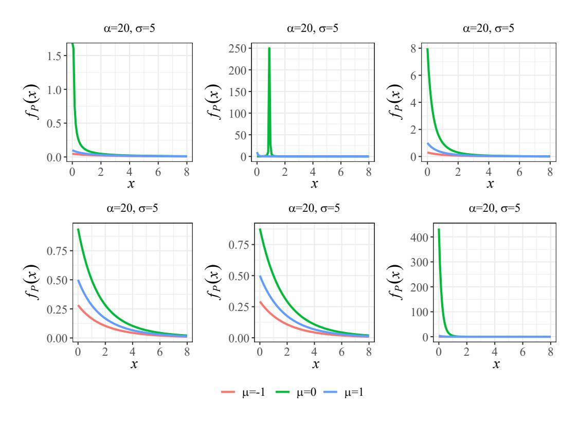
Figure 1: Examples of Generalized Pareto Type II density functions varying the values of the parameters.
Meanwhile, the pdf of the Weibull distribution with parameters κ > 0 (shape) and λ > 0 (scale), is defined for x > 0 as
\[f_W(x) = \frac{\kappa}{\lambda} \left(\frac{x}{\lambda}\right)^{\kappa-1} \exp\left[-\left(\frac{x}{\lambda}\right)^{\kappa}\right].\] (7)
The objective of this paper is to study some properties of Pareto graphs defined as those graphs for which their degree distribution follows a GPDII with µ = 0. Section §2 is devoted to deducing a way to compute the generating function for the component sizes and give sufficient conditions for the presence or absence of a giant component. Section §3 presents the results of a simulation study to generate Pareto random graphs varying the values of the parameters. This approach includes the percentage of right generation, as well as some local and global metrics in the approximation of the degree probabilities. Moreover, a simulation is conducted to study some properties related to the connectivity of a random graph generated by different models. Section §4 contains applications to real-world social networks and the assessment of the goodness of fit compared with other heavytailed degree distributions. Finally, in Section §5 we include some concluding remarks.
2. Pareto graphs
We say that a random graph is a Pareto graph if the degree distribution follows a Generalized Pareto Distribution of Type II with µ = 0. If we call X ∼ GP DII the variable that models the
degree distribution, applying the Right Riemann sum, we have that
\[p_{k} = P(X = k) = P(k \le X < k+1) = F_{P}(k+1) - F_{P}(k) =\] \[= 1 - \left(1 + \frac{k+1}{\sigma}\right)^{-\alpha} - 1 + \left(1 + \frac{k}{\sigma}\right)^{-\alpha} = \sigma^{\alpha}[(\sigma + k)^{-\alpha} - (\sigma + k+1)^{-\alpha}].\] (8)
It is clear that pk > 0 for all non-negative integer k.
In this case, the generating function for x ≥ 0 is
\[G_0(x) = \sigma^{\alpha} \sum_{k=0}^{+\infty} [(\sigma + k)^{-\alpha} - (\sigma + k + 1)^{-\alpha}] x^k.\] (9)
Notice the following
\[G_0(1) = \sum_{k=0}^{+\infty} p_k = \sum_{k=0}^{+\infty} F_P(k+1) - F_P(k) =\] \[= \lim_{n \to +\infty} \sum_{k=0}^{n} F_P(k+1) - F_P(k) = \lim_{n \to +\infty} F_P(n+1) - F_P(0).\] (10)
Since FP (0) = 0 and limx→+∞ FP (x) = 1 by cdf properties, it holds that G0(1) = 1. Moreover, by derivation
\[G_0'(x) = \sigma^{\alpha} \sum_{k=1}^{+\infty} k [(\sigma + k)^{-\alpha} - (\sigma + k + 1)^{-\alpha}] x^{k-1},\] (11)
which implies that
\[G_0'(1) = \sigma^{\alpha} \sum_{k=1}^{+\infty} k[(\sigma + k)^{-\alpha} - (\sigma + k + 1)^{-\alpha}] = \sigma^{\alpha} \sum_{k=1}^{+\infty} \frac{1}{(\sigma + k)^{\alpha}}.\] (12)
By comparison with p-series, G′ 0 (1) is well defined if α > 1. Hence, replacing in (2) by the expression obtained in (12),
\[G_1(x) = \frac{1}{\eta} \sum_{k=1}^{+\infty} k[(\sigma + k)^{-\alpha} - (\sigma + k + 1)^{-\alpha}]x^{k-1},\] (13)
where η = P+∞ k=1(σ + k) −α .
2.1. Component sizes
A connected component of an undirected graph is a subgraph in which any two vertices are connected to each other by a collection of edges, but no vertex in the component can have an edge to another component. The size of a graph is defined as the number of edges (see for instance [13]). The largest component of a graph is called its giant component, which is a unique
and distinguishable component containing a significant fraction of all the vertices dwarfing all the other components [18].
Using that all components in the infinite configuration model are locally tree-like, the authors in [15], showed that there exists a correspondence between the distributions of the degrees and the component sizes by applying generation functions. More precisely, let \(H_1(x)\) be the generating function for the distribution of the sizes of components that are reached by choosing a random edge and following it to one of its ends. If there exists a giant component, we exclude it from \(H_1(x)\).
Let \(q_k\) be the probability that the initial site has k edges coming out of it other than the edge we came in along. Applying the "powers" property, \(H_1(x)\) must satisfy a self-consistency condition of the form
\[H_1(x) = \sum_{k} x q_k [H_1(x)]^k.\] (14)
Note that each such component is associated with the end of an edge. If \(H_0 = \sum_{n=1}^{+\infty} h(n)x^n\) is the generating function for the size of the whole component and realizing that \(q_k\) is the coefficient of \(x^k\) in the generating function \(G_1(x)\), we have the following system of equations
\[\begin{cases} H_0(x) = xG_0(H_1(x)), \\ H_1(x) = xG_1(H_1(x)). \end{cases}\] (15)
We can apply the Lagrange inversion formula [2] to solve (15). This method says that if A(x) and R(x) are formal power series satisfying that
\[A(x) = xR(A(x)), (16)\]
then for a formal power series F(x), it holds that
\[[x^n]F(A(x)) = \frac{1}{n}[t^{n-1}]F'(t)R^n(t), \tag{17}\]
where \([x^n]S(x)\) indicates the coefficient of \(x^n\) in the formal series S(x). Considering \(A(x) = H_1(x)\), \(R(x) = G_1(x)\) and \(F(x) = G_0(x)\), for n > 1 it holds that
\[h(n) = [x^{n-1}]G_0(H_1(x)) = \frac{1}{n-1}[t^{n-2}]G_0'(t)G_1^{n-1}(t) = \frac{1}{n-1}[t^{n-2}]G_0'(1)G_1^n(t).\] (18)
This, applying (2) and (12), we conclude that if \(\alpha > 1\), then
\[h(n) = \frac{\sigma^{\alpha} \eta}{n-1} [t^{n-2}] G_1^n(t).\] (19)
However, there are limits in searching for an exact solution of (19), even if performing numerical computations, due to the complexity of the generating functions in the case of Pareto graph. Theses difficulties arise because of the implementation of the inverse generation function transform. In [11], the author rewrites (19) using the concept of convolution power.
Recall that for two distributions f and g, we can define a binary multiplicative operation for k > 0 as follows
\[f(k) * g(k) = \sum_{i=0}^{k} f(i)g(k-i).\] (20)
Moreover, the convolution given in (20) can be inductively extended to the convolution power in the following manner:
\[f(k)^{*n} = f(k)^{*n-1} * f(k), (21)\]
where f(k) ∗0 = 1 by definition.
Now, using the results obtained in [11], the general expression for the component size distribution for Pareto graphs looks like
\[h(n) = \begin{cases} \frac{[kF_P(k+1) - kF_P(k)]^{*n}(2n-2)}{(n-1)(\eta\sigma^{\alpha})^{n-1}} (2n-2) & \text{if } n > 1, \\ F_P(1) & \text{if } n = 1. \end{cases}\](22)
Let α > 1, we present the first four values of h(n) to show the complexity of the form as n increases:
\[h(1) = F_P(1) = 1 - \sigma^{\alpha}(\sigma + 1)^{-\alpha},\] \[h(2) = \frac{1}{\eta \sigma^{\alpha}} [F_P(2) - F_P(1)]^2\] \[= \frac{\sigma^{\alpha}}{\eta} [(\sigma^2 + 2\sigma + 1)^{-\alpha} + (\sigma^2 + 4\sigma + 4)^{-\alpha} - 2(\sigma^2 + 3\sigma + 2)^{-\alpha}],\] \[h(3) = \frac{1}{2(\eta \sigma^{\alpha})^2} 6[F_P(2) - F_P(1)]^2 [F_P(3) - F_P(2)] =\] \[= \frac{3\sigma^{\alpha}}{\eta^2} [(\sigma^3 + 6\sigma^2 + 12\sigma + 8)^{-\alpha} + (\sigma^3 + 4\sigma^2 + 5\sigma + 2)^{-\alpha} - (\sigma^3 + 5\sigma^2 + 7\sigma + 3)^{-\alpha} - 2(\sigma^3 + 5\sigma^2 + 8\sigma + 4)^{-\alpha} - (\sigma^3 + 7\sigma^2 + 16\sigma + 12)^{-\alpha} + 2(\sigma^3 + 6\sigma^2 + 11\sigma + 6)^{-\alpha}],\]
\[h(4) = \frac{1}{3(\eta\sigma^{\alpha})^{3}} \{12[F_{P}(2) - F_{P}(1)]^{3}[F_{P}(4) - F_{P}(3)] + 24[F_{P}(2) - F_{P}(1)]^{2}[F_{P}(3) - F_{P}(2)]^{2}\} =\] \[= \frac{4\sigma^{\alpha}}{3\eta^{3}} [2(\sigma^{4} + 8\sigma^{3} + 24\sigma^{2} + 32\sigma + 16)^{-\alpha} + (\sigma^{4} + 6\sigma^{3} + 12\sigma^{2} + 10\sigma + 3)^{-\alpha} - (\sigma^{4} + 7\sigma^{3} + 15\sigma^{2} + 13\sigma + 4)^{-\alpha} - 4(\sigma^{4} + 7\sigma^{3} + 18\sigma^{2} + 20\sigma + 8)^{-\alpha} - 5(\sigma^{4} + 9\sigma^{3} + 30\sigma^{2} + 44\sigma + 24)^{-\alpha} + (\sigma^{4} + 10\sigma^{3} + 36\sigma^{2} + 56\sigma + 32)^{-\alpha} + 2(\sigma^{4} + 6\sigma^{3} + 13\sigma^{2} + 12\sigma + 4)^{-\alpha} + 2(\sigma^{4} + 8\sigma^{3} + 20\sigma^{2} + 24\sigma + 9)^{-\alpha} + 2(\sigma^{4} + 10\sigma^{3} + 37\sigma^{2} + 60\sigma + 36)^{-\alpha} - 7(\sigma^{4} + 7\sigma^{3} + 17\sigma^{2} + 17\sigma + 6)^{-\alpha} + 3(\sigma^{4} + 8\sigma^{3} + 21\sigma^{2} + 22\sigma + 8)^{-\alpha} + 11(\sigma^{4} + 8\sigma^{3} + 23\sigma^{2} + 28\sigma + 12)^{-\alpha} - 3(\sigma^{4} + 9\sigma^{3} + 28\sigma^{2} + 36\sigma + 16)^{-\alpha}].\]
2.2. Giant component
Throughout this section, we consider a Pareto graph with degree distribution given as in (3) with µ = 0 and α > 1.
In [15] the authors prove that the phase transition at which a giant component first appears is given when G′ 1 (1) = 1. This fact implies a necessary and sufficient condition for the existence of a giant component which settles that
\[\sum_{k} k(k-2)p_k > 0. (23)\]
For Pareto graphs, using (8), we can simplify (23) to the following form
\[\sum_{k} k(k-2)[(\sigma+k)^{-\alpha} - (\sigma+k+1)^{-\alpha}] > 0 \iff \underbrace{\sum_{k=1}^{+\infty} \frac{k(k-2)}{(\sigma+k)^{\alpha}}}_{S_1} - \underbrace{\sum_{k=1}^{+\infty} \frac{k(k-2)}{(\sigma+k+1)^{\alpha}}}_{S_2} > 0. (24)\]
In order to obtain a simpler form of this inequality, we can observe that
- the term with denominator (σ + 1)α only appears in S1 with coefficient −1,
- the term with denominator (σ + 2)α only appears in S2 with coefficient 1,
- the term with denominator (σ + 3)α only appears in S1 with coefficient 3.
- the term with denominator (σ + k) α for k ≥ 4 appears in both S1 and S2 with coefficient k(k − 2) − (k − 1)(k − 3) = 2k − 3.
Thus, the next result follows immediately.
Corollary 2.1. There exists a giant component in a Pareto graph if and only if P+∞ k=1 2k−3 (σ+k)α is positive. (Notice that the only negative term in this sum appears when k = 1.)
Proposition 2.1. For fixed values α, σ ∈ R+, we consider f(x) = (2x − 3)(σ + x) −α . If α > 1 and 3α < ln(5)σ, then f(4) > −f(1).
Proof. Notice that
\[f(4) > -f(1) \Longleftrightarrow \frac{5}{(\sigma+4)^{\alpha}} > \frac{1}{(\sigma+1)^{\alpha}} \Longleftrightarrow \sigma > \frac{4-5^{1/\alpha}}{5^{1/\alpha}-1}.\] (25)
We are going to prove that
\[\frac{4 - 5^{1/\alpha}}{5^{1/\alpha} - 1} < \frac{3}{\ln(5)}\alpha \Longleftrightarrow \left(\frac{3\alpha + 4\ln(5)}{3\alpha + \ln(5)}\right)^{\alpha} < 5. \tag{26}\]
Since the left-hand side of the second inequality in (26) defines a monotonous decreasing function of α whose limit to positive infinity is equal to 5, the mentioned inequality is satisfied, and so (25) is also true by the hypothesis 3α < ln(5)σ.
Corollary 2.2. If a Pareto graph is such that 3α < ln(5)σ, then there exists a giant component.
Proof. It is straightforward by Proposition 2.1 and Corollary 2.1.
Proposition 2.2. If σ ≥ α, then there exists a giant component for a Pareto graph.
Proof. Consider the function
\[g(x) = \frac{1}{(x+2)^x} + \frac{3}{(x+3)^x} + \frac{5}{(x+4)^x} - \frac{1}{(x+1)^x}.\] (27)
Thus,
\[g'(x) = \frac{(x+1)\ln(x+1) + x}{(x+1)^{x+1}} - \frac{(x+2)\ln(x+2) + x}{(x+2)^{x+1}} - 3\frac{(x+3)\ln(x+3) + x}{(x+3)^{x+1}} - 5\frac{(x+4)\ln(x+4) + x}{(x+4)^{x+1}}.\] (28)
Applying specific software, we can see that g ′ (x) is continuous and negative in [0, +∞), as shown in Figure 2. This implies that g(x) is monotonous decreasing in [0, +∞). Moreover, limx→+∞ g(x) = 0 and g(0) = 8 > 0. By continuity, g(x) > 0 for all x ≥ 0.
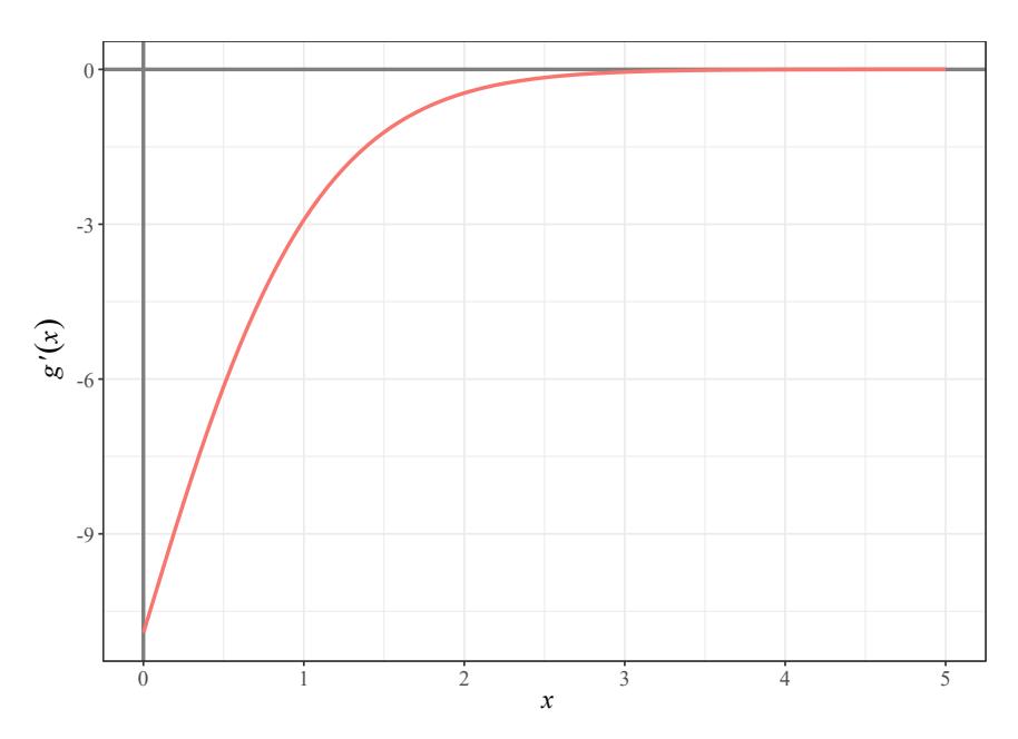
Figure 2: Plot of the derivative of g(x) given in (28).
Suppose now that α = σ. In this case, g(α) represents the sum of the first four terms in the sum given in Corollary 2.1 that has been proved to be positive. As a consequence, there exists a giant component for a Pareto graph with α = σ.
If σ > α, then σ = α + b with b > 0. This change produces horizontal shifts of the function g(x), as it is displayed in Figure 3. Hence, the sign of g(x) remains positive and we can also prove the presence of a giant component in an analogous way as above.
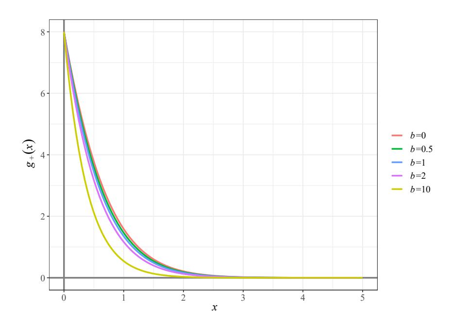
Figure 3: Examples of horizontal shifts of the function g(x) given in (27), considering different values of b in the function \(g_+(x) = (x+b+2)^{-x} + 3(x+b+3)^{-x} + 5(x+b+4)^{-x} - (x+b+1)^{-x}\).
Proposition 2.3. If \(\alpha > 4\) and \(2\sigma \le \alpha - 4\), then there is no giant component for a Pareto graph.
Proof. We consider the function f(x) given in 2.1. Hence,
\[f'(x) = 0 \Longleftrightarrow \frac{2(\sigma + x) - \alpha(2x - 3)}{(\sigma + x)^{\alpha + 1}} = 0 \Longleftrightarrow x = \frac{3\alpha + 2\sigma}{2\alpha - 2}.\] (29)
Notice that the denominator in f'(x) is always positive and the numerator is represented by a linear function with a negative gradient so that the critical point obtained in (29) is a maximum of f(x).
The hypothesis \(2\sigma \le \alpha - 4\) says that the maximum value of f(x) is achieved at \(x_0 \le 2\). Thus, if \(a_k = f(k)\), \((a_k)_{k \ge 2}\) is a decreasing succession of positive terms and
\[\sum_{k=3}^{+\infty} a_k < \int_2^{+\infty} f(x)dx = \lim_{b \to +\infty} \left[ \frac{2x - 3}{(1 - \alpha)(\sigma + x)^{\alpha - 1}} - \frac{2}{(1 - \alpha)(2 - \alpha)(\sigma + x)^{\alpha - 2}} \right] \Big|_2^b\] \[= \frac{2}{(1 - \alpha)(2 - \alpha)(\sigma + 2)^{\alpha - 2}} - \frac{1}{(1 - \alpha)(\sigma + 2)^{\alpha - 1}}\] \[= \frac{2 + \alpha + 2\sigma}{(1 - \alpha)(2 - \alpha)(\sigma + 2)^{\alpha - 1}}.\] (30)
Therefore,
\[\sum_{k=1}^{\infty} a_k < \frac{2+\alpha+2\sigma}{(1-\alpha)(2-\alpha)(\sigma+2)^{\alpha-1}} + \underbrace{\frac{1}{(\sigma+2)^{\alpha}}}_{a_2} \underbrace{-\frac{1}{(\sigma+1)^{\alpha}}}_{a_1} := u(\alpha,\sigma). \tag{31}\]
The right hand side in (31) defines a function u(α, σ) that takes values under zero on the region {(α, σ) ∈ R2/α > 4, 0 < σ ≤ (α − 4)/2}, as it is exhibit in Figure 4. It is clear now that the condition of Corollary 2.1 is false and so, it is impossible that a giant component arises.
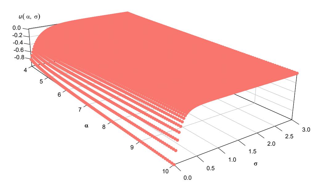
Figure 4: Plot of the function u(α, σ) defined in the right hand side of (31) in the domain defined by the hypothesis of Proposition 2.3 .
We summarize the previous results for Pareto graphs in Figure 5, where the zones colored in green point to the existence of a giant component, meanwhile, the red ones correspond to the absence of giant components. The isolated points are examples of manual proof selected to illustrate other cases.
3. Simulation
This section is devoted to presenting two types of simulation. In the first stage, we study the performance of Pareto graph generation providing an assessment of its efficacy and describing some observed properties. The second stage concerns comparing some characteristics of random graphs generated by different models.
3.1. Pareto graph generation behavior
We perform our experiment for graphs with n vertices considering n = 10, 50, 100, 1000. We chose as possible vertex degrees those in the interval [0, b] varying b = 1, 2, 4, 6, 10, 20. Finally, we set the GPDII parameters as µ = 0, α = 1.1, 2, 5, 10, 20, and σ = 1, 2, 5, 10, 20. In this election, we are considering different types of textures for SAR images.
For each of these parameter combinations and each degree interval vertex, we generated R = 1000 GPDII sequences of n degrees in the correspondent interval applying the rejection method.
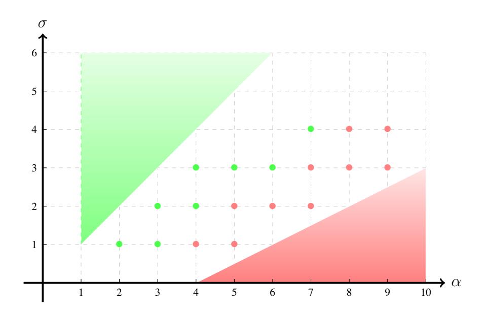
Figure 5: According to the values of the parameters for a Pareto graph, regions for which a giant component exists are indicated in green, and regions where a giant component does not exist are marked in red.
Then, for each of these degree sequences, we generated a random graph whose vertices respect the degrees in the sequence and we then computed the degree distribution using the <code>igraph</code> library [5] from R. Since the existence of such graphs is guaranteed as long as the sum of all the degrees is even, we computed the percentage of right graph generation, named efficacy. Due to the GPDII asymptotic behavior (cf. Figure 1), we also registered the absence of some degrees in the simulations.
Taking into account the efficacy in the graph generation, we worked with balanced samples of size 450 for each combination of parameters. Let \(\widehat{f}(k)\) be the obtained approximation to the degree distribution f(k), we found the following metrics:
- the bias at the point k, defined by \(\mathrm{E}[\widehat{f}(k)] f(k)\), where \(\mathrm{E}[\cdot]\) denotes the expected value,
- the variance at the point k, defined by \(\mathrm{E}\{\widehat{f}(k) \mathrm{E}[\widehat{f}(k)]\}^2\),
- the \(L_{\infty}\) norm or sup absolute error (SAE), defined by \(SAE[\widehat{f}(k)] = \sup_{k} |\widehat{f}(k) f(k)|\). This global measure enables us to obtain an estimation and representation of the whole density in this case we are using a non-parametric estimation.
In the first trials, we also considered the case \(\sigma=0.1\) which was aborted because it showed problems when applying the rejection method due to the enormous maximum value the pdf takes in the degree intervals, (cf. Figure 1).
In terms of the efficacy of the generation, we observed that it is similar for all the considered numbers of vertices, except for
• \[\alpha=5\] and \(\sigma=1\), • \(\alpha=10\) and \(\sigma=2\), • \(\alpha=20\) and \(\sigma=5\),
where the percentage of efficacy is extremely better if n = 10. The degree interval seems to make no difference either.
We had a very good performance (even up the 90%) when:
• \[\alpha=10\] and \(\sigma=1\), • \(\alpha=20\) and \(\sigma=1,2\).
The performance is acceptable (between 75% and 90%) for n = 10 when:
• \[\alpha=5\] and \(\sigma=1\), • \(\alpha=10\) and \(\sigma=2\).
For the rest of the cases, the percentage of generation efficacy is between 45% and 60%. These features are exhibited in Figure 6 which shows the percentage of the efficacy in the graph generation, where the gray and grey dotted horizontal lines represent 90% and 75%, respectively.
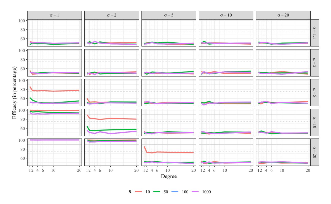
Figure 6: Percentage of efficacy in the generation of Pareto graph with n vertices, according to the values of the distribution parameters.
We could see that in the following cases, the obtained graphs are conformed by isolated points, i.e. all the vertices have degree zero:
• \[\alpha = 10\], \(\sigma = 1\), and \(n = 10\),
• \[\alpha = 20\], \(\sigma = 1\), for all values of \(n\),
• \[\alpha = 20\], \(\sigma = 2\), and \(n = 10, 50\).
As the upper limit of the degree interval increases, the absence of high degrees is notorious for big values of α and small values of σ. We illustrate this phenomenon in Figure 7 in which we mark the degrees that do not appear in the generated random graphs.
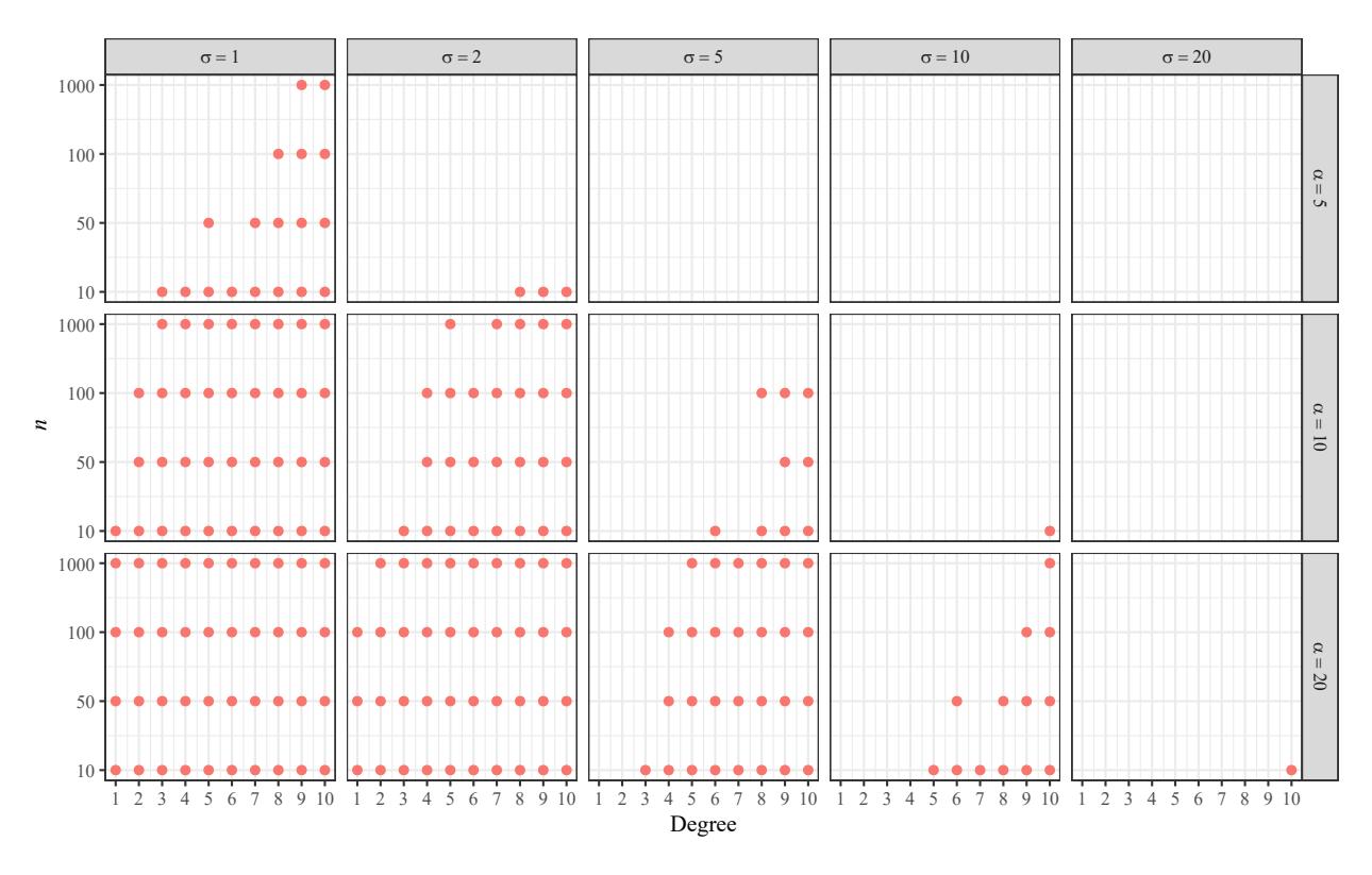
Figure 7: Missed degrees in the interval [0, 10] when generating a Pareto random graph with n vertices, according to the different values of the distribution parameters.
Figure 8 represents one of the graphics we used to analyze the error produced when approximating the probability that a vertex has a degree equal to k using the generated random graphs. In this figure, we plot the biases where the pairs denote the values (α, σ) and p(k) is the probability that a vertex has a degree equal to k.
After this study, we observed the following:
- The differences in the results are imperceptible to the variation in the amount of vertices in the graph.
- The largest biases come from overestimation.
- The biases are very small, ordering from least to greatest, when
Pareto graphs | Andrea Rey
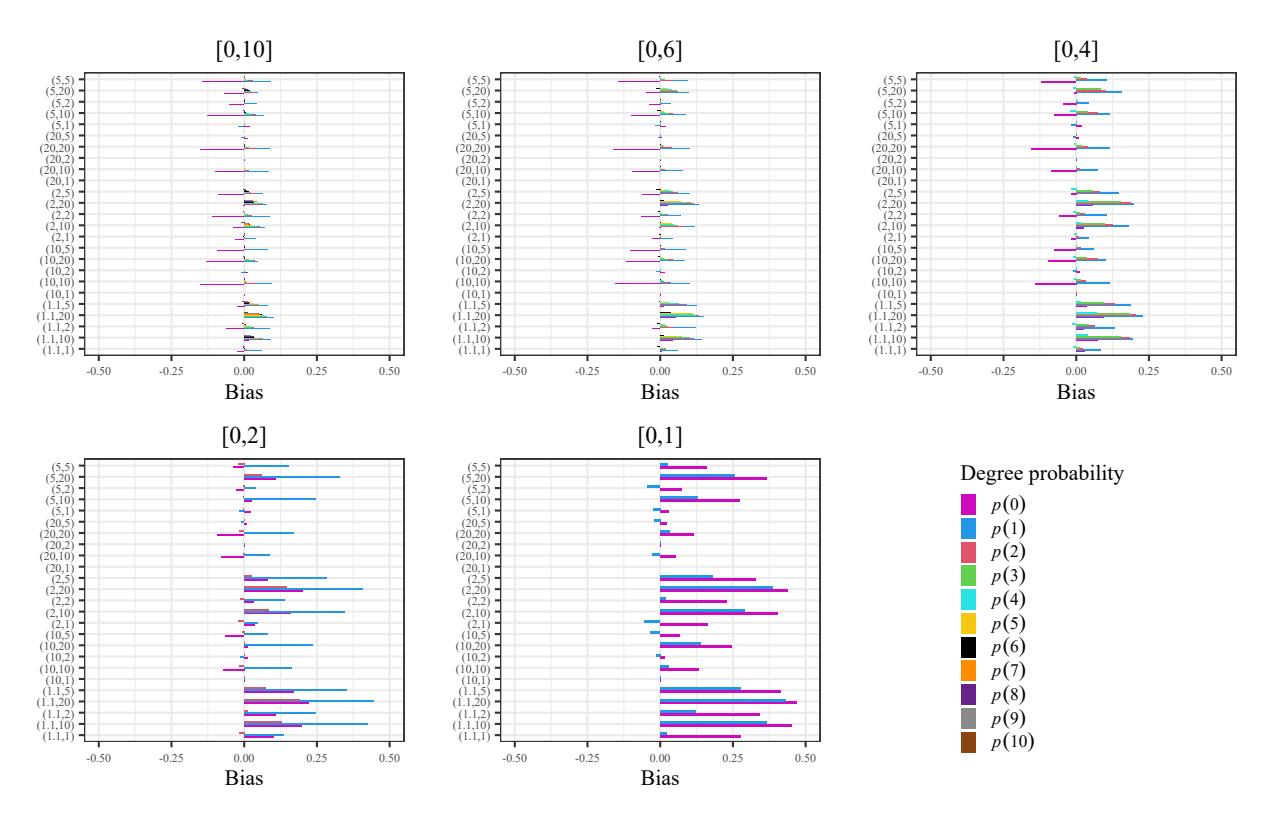
Figure 8: Some examples of the biases in the degree distribution for Pareto graph generation with 10 vertices, according to the values of the distribution parameters and the interval [0, b] for the allowed degrees.
- \[\alpha=20\] and \(\sigma=1\), - \(\alpha=10\) and \(\sigma=1\), - \(\alpha=20\) and \(\sigma=2\).
- In general we can see that the worst approximations hold for smaller degrees.
- In Figure 9 we sum up the cases for which the approximation is not so good.
We choose Figure 10 as an example to introduce the tools employed in the variance study, with the same notation as above.
We point out the following features:
- For graphs that are trees; i.e. each vertex has only degree 0 or 1, the variances for these degrees are similar. On the other hand, the variance decreases as the degree increases.
- If we notice by \(\Upsilon_n\) the upper bound for the variance in the n-vertex graph generation, we see that \(\Upsilon_{10}=0.025,\ \Upsilon_{50}=10^{-1}2\Upsilon_{10},\ \Upsilon_{100}=10^{-1}\Upsilon_{10}\) and \(\Upsilon_{1000}=10^{-2}\Upsilon_{10}\). So that the variance declines as the number of vertices grows.
- In Figure 11 we exhibit all the cases in which the variance is almost insignificant. In the analysis of the SAE, we refer to Figure 12 to conclude the following:
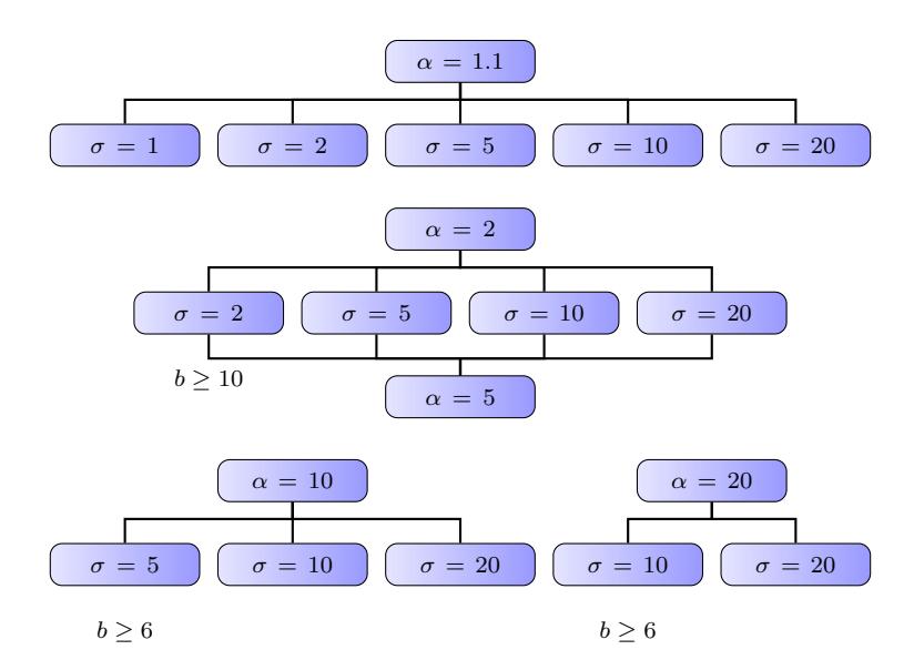
Figure 9: Combinations of distribution parameters in which the degree distribution approximation biases are unsatisfactory.
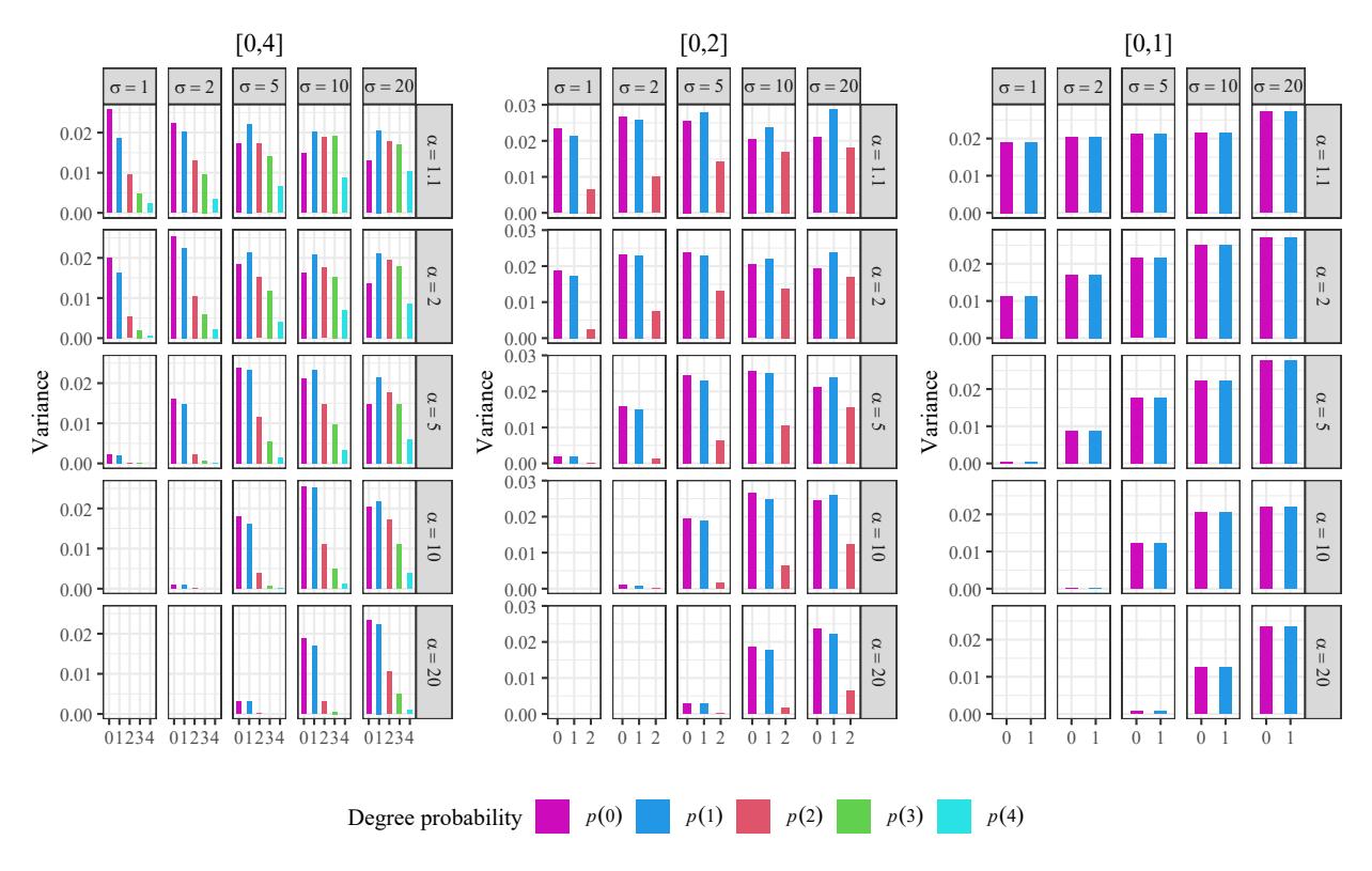
Figure 10: Some examples of the variance in the degree distribution for Pareto graph generation with 10 vertices, according to the values of the distribution parameters and the interval [0, b] for the allowed degrees.
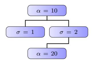
Figure 11: Combinations of distribution parameters in which the variance produced in the estimation of degree distribution is negligible.
- The SAE is low for \(\alpha=1.1\) and \(\sigma=1,2,5\); except for large degrees in the case n=50.
- The SAE is low for \(\alpha=1.1\) and \(\sigma=10,20\); when the degrees are not small, except in the case n=50.
- The SAE is acceptable when \(\alpha=2\), except for n=50 considering small values of \(\sigma\) and big degrees.
- In general, the SAE is near to one for \(\alpha = 5, 10, 20\).

Figure 12: SAE computation for all the cases considered in the simulation study.
3.2. Graph generation models comparison
In this experiment, for the number of vertices n=5,10,50, we generated R=1000 undirected random graphs with possible loops, using the following models:
- ER: Erdos and R ˝ enyi with probability ´ p = 0.5 for the creation of each possible new edge, by using the function sample gnp in R.
- BA: Scale-Free Barabasi and Albert with power ´ ω = 1, by using the function sample pa in R.
- P1: Pareto graph by applying the rejection method in the interval [0, 10] with parameters µ = 0, α = 1, and σ = 3.
- P2: Pareto graph by applying the rejection method in the interval [0, 10] with parameters µ = 0, α = 1, and σ = 5.
- P3: Pareto graph by applying the rejection method in the interval [0, 10] with parameters µ = 0, α = 2, and σ = 2.
For illustrative purposes, Figure 13 shows the appearance of a graph generated by each one of these models and varying the number of vertices.
For each model and for each n, we computed the following:
- percentage of connected and non-connected graph (Table 1 shows these results),
- number of connected components in the graph (Figure 14 shows the distribution of these amounts),
- number of isolated nodes in the graph, i.e. vertices with a null degree, (Figure 15 shows the distribution of these amounts).
| Table 1: Percentage of connected (C) and non-connected (NC) graphs with n vertices in each group. | |
|---|---|
| Model | ||||||||||
|---|---|---|---|---|---|---|---|---|---|---|
| ER | BA | P1 | P2 | P3 | ||||||
| C | NC | C | NC | C | NC | C | NC | C | NC | |
| n = 5 | 69.1 | 30.9 | 100.0 | 0.0 | 23.4 | 76.6 | 35.8 | 64.2 | 3.0 | 97.0 |
| n = 10 | 98.1 | 1.9 | 100.0 | 0.0 | 7.6 | 92.4 | 18.5 | 81.5 | 0.1 | 99.9 |
| n = 50 | 100.0 | 0.0 | 100.0 | 0.0 | 0.0 | 100.0 | 0.1 | 99.9 | 0.0 | 100.0 |
It is observed that as the number of vertices increases the number of connected Erdos-R ˝ enyi ´ and Barabasi-Albert graphs also increases. On the other hand, the number of connected Pareto ´ graphs, as well as the number of isolated nodes in this kind of graph, decreases. This is a clear consequence of the heavy-tailed condition satisfied by the Pareto distribution. The behavior of these features is similar for random graphs generated by the models ER and BA.
Pareto graphs | Andrea Rey
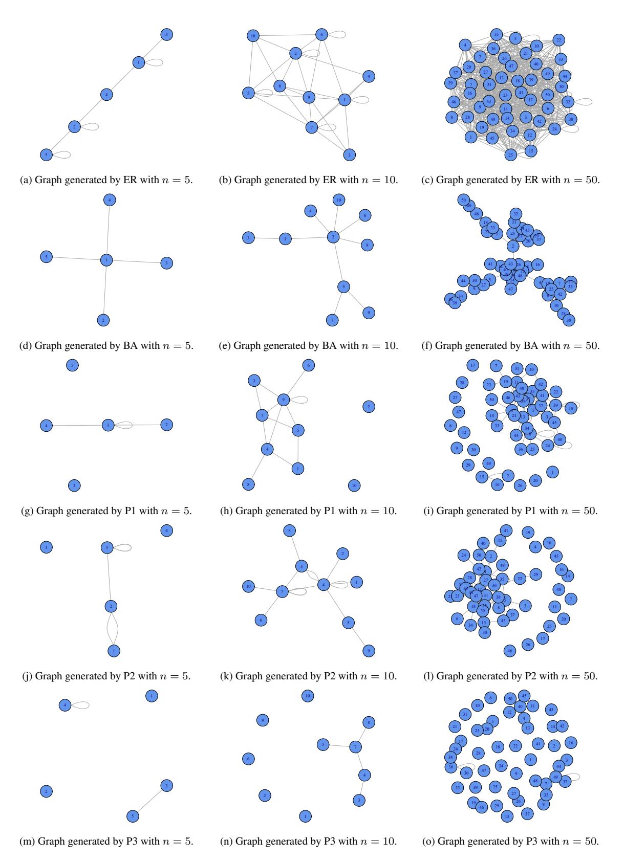
Figure 13: Random graph with n vertices generated by different models.
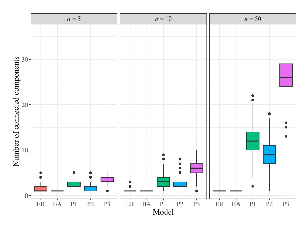
Figure 14: Distribution of the number of components in n-vertex random graphs generated by different models.
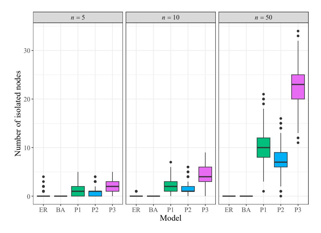
Figure 15: Distribution of the number of isolated nodes in n-vertex random graphs generated by different models.
4. Application to real social networks
All the data we use in this section are obtained from [21].
Emphasizing the application of graphs to real-world systems, the term network is sometimes defined to mean a graph in which the attributes are associated with the vertices and the edges. For instance, the vertices can be the names of the people belonging to a social group, meanwhile, the edges represent some kind of interconnection among them. Particularly, we are going to work with the following social networks:
- Brightkite was a location-based social networking website in which users were able to check in at places by using text messaging or one of the mobile applications and they were able to see who was nearby and who had been there before. The service was created in 2007 by Brady Becker, Martin May, and Alan Seideman who previously founded the SMS notification service Loopnote. In April 2009 Brightkite was acquired by the mobile social network Limbo. The dataset contains all links among users.
- Hamsterster is about the friendships and family links between users of an intended ironically website for tailless rodents. The dataset contains all friendships among the users.
- Wikipedia is a free encyclopedia written collaboratively by volunteers around the world. The dataset contains all the Wikipedia voting data from the creation of Wikipedia till January 2008, where a directed edge from node i to node j represents that user i voted on user j.
In the whole analysis we implement the software R [19]. We obtained graphs from the data with the function graph.edgelist from library igraph [5]. The number of vertices and edges of each graph appears in Table 2.
| Graph | Vertices | Edges | Type |
|---|---|---|---|
| Brightkite | 56739 | 212944 | Undirected |
| Hamsterter | 2426 | 16629 | Undirected |
| Wikivote | 889 | 2913 | Directed |
Table 2: Dataset graph information.
We use the function fitgpd from library POT [20] which returns the parameters optimized and fixed, selecting the maximum likelihood estimator. In this package, the Generalized Pareto distribution function, for loc = u, scale = σ and shape = ξ is given by
\[G(x) = 1 - \left[1 + \frac{\xi(x-u)}{\sigma}\right]^{-1/\xi} \tag{32}\]
for 1 + ξ(x − u)/σ > 0 and x > u, where σ > 0.
We estimate the parameters in (3) as follows:
• µb is the minimum value of the degrees in the graph,
- αb is the inverse of the shape parameter in (32),
- σb is the quotient between the scale and the shape parameters in (32).
In addition, we estimate the parameters involved in the pdf of the Log-Normal and Weibull distributions, given in (6) and (7), respectively. These estimations were computed using the functions elnorm for the Log-Normal distribution and eweibull for the Weibull distribution, from the package EnvStats [14]. The obtained estimated values are in Table 3.
| Distribution | |||||||
|---|---|---|---|---|---|---|---|
| Graph | Pareto | Log-Normal | Weibull | ||||
| µ b | α b | σ b | µ bℓ | σ bℓ | κ b | λb | |
| Brightkite | 1 | 1.91340 | 9.23148 | 1.12612 | 1.15066 | 0.73815 | 5.72488 |
| Hamsterter Wikivote | 1 1 | 3.35064 6.04307 | 34.34426 35.59667 | 1.92937 1.34905 | 1.18774 1.00655 | 0.85954 0.96956 | 12.51456 6.44806 |
Table 3: Parameter estimation for heavy-tailed distributions.
In Figure 16, we visually compare the empirical degree distribution obtained by applying the function degree distribution from library igraph lighted in green, with the Pareto, Log-Normal, and Weibull distributions defined by the estimation of the parameters given in Table 3. The three distributions seem to properly fit the real data. Since these distributions correspond to continuous random variables and the degrees are discrete, we compute the mean square error (MSE) to assess the goodness of fit with a quantitative measure. The MSE was computed as
\[MSE = \sum_{k=1}^{30} [p_k - f_{\mathcal{D}}(k)]^2,\] (33)
where pk is the empirical probability of the degree k and D ∈ {P, LN, W}. The results are shown in Table 4, where the best values are in bold.
Table 4: Mean square errors between the observed degree distribution and heavy-tailed distributions.
| Graph | Pareto | Log-Normal | Weibull |
|---|---|---|---|
| Brightkite | 0.02552 | 0.20913 | 0.04347 |
| Hamsterter | 0.00194 | 0.00226 | 0.003464 |
| Wikivote | 0.00427 | 0.00436 | 0.00947 |
Moreover, the parameters of the Pareto distribution, which are presented in Table 3, verify the hypothesis of Proposition 2.2 which implies that there is a giant component in the three graphs considered.
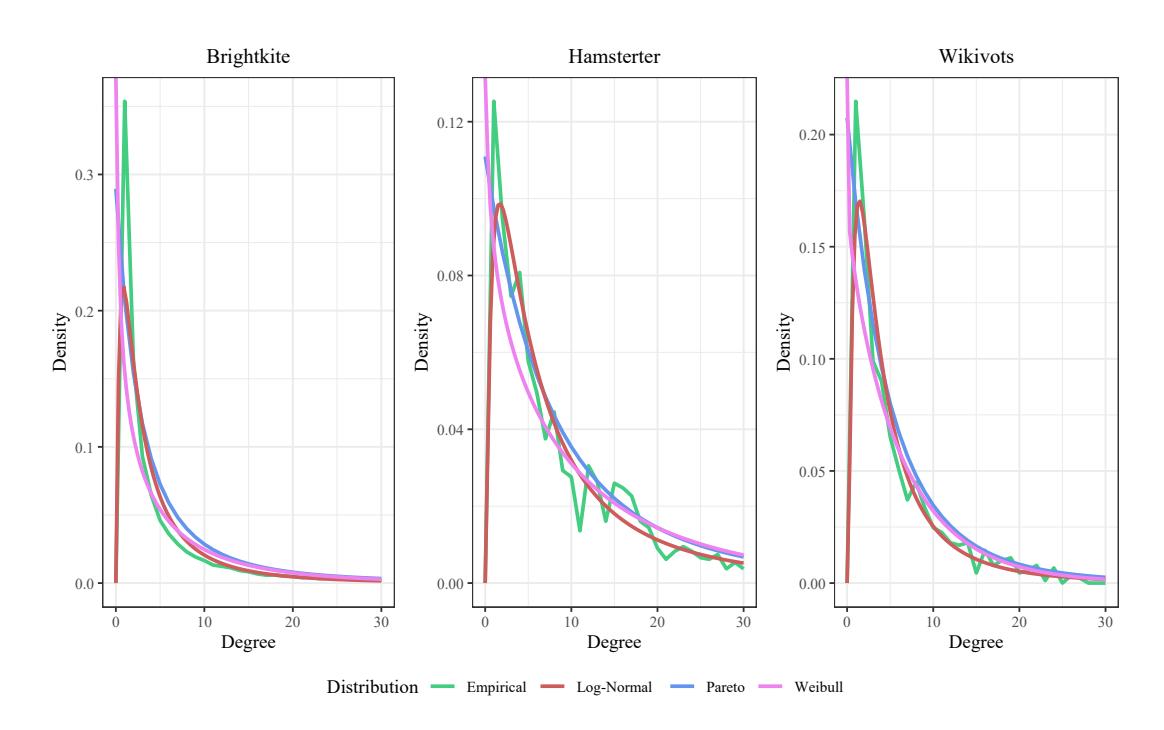
Figure 16: Heavy-tailed distribution approximation to the degree distribution in real social networks.
5. Conclusions and remarks
Due to the results obtained in Section §2, we can think that the existence of a giant component is conditioned to the division into two semi-planes of the first quadrant given by the parameters α and σ when dealing with Pareto graphs.
The simulation results indicate a good performance in graph generation for the combination of large values of α and small values of σ. On the contrary, the global error in the approximations is acceptable when α takes small values. In general, the variance is very small, even depreciated for small values of σ meanwhile, α takes large values.
The Generalized Pareto Distribution of Type II showed the best fit (measured by the mean square error) for two of the three real-world networks for which it was applied and proved to be competitive with the Log-Normal distribution in the remaining case. Another advantage to using the Pareto distribution to model real-world networks whose degrees follow a heavy-tailed distribution is that the associated probability density function requires less computational cost due to the simplicity of the involved operations.
References
- [1] A.L. Barabasi and R. Albert, Emergence of scaling in random networks, ´ Science, 286(5439) (1999), 509–512.
- [2] F. Bergeron, G. Labelle, and P. Leroux, Combinatorial Species and Tree-Like Structures, Cambridge University Press, 67, 1998.
Pareto graphs | Andrea Rey
- [3] B. Bollobas and B. B ´ ela, ´ Random Graphs, Cambridge University Press, 73, 2001.
- [4] D.G. Champernowne, A model of income distribution, The Economic Journal, 63(250) (1953), 318–351.
- [5] G. Csardi and T. Nepusz, The igraph software package for complex network research, Inter-Journal Complex Systems, 1695 (2006), 1–9.
- [6] P. Erdos and A. R ˝ enyi, On random graphs I, ´ Publ. Math. Debrecen, 6 (1959), 290–297.
- [7] P. Erdos and A. R ˝ enyi, On the evolution of random graphs, ´ Publ. Math. Inst. Hungar. Acad. Sci, 5 (1960), 17–61.
- [8] P. Erdos and A. R ˝ enyi, On the strength of connectedness of a random graph, ´ Acta Mathematica Hungarica, 12(1-2) (1961), 261–267.
- [9] A.C. Frery, H.J. Muller, C. da Costa Freitas Yanasse, and S.J. Siqueira Sant'Anna, A model for extremely heterogeneous clutter, IEEE Transactions on Geoscience and Remote Sensing, 35(3) (1997), 648–659.
- [10] C.M. Harris, The Pareto distribution as a queue service discipline, Operations Research, 16(2) (1968), 307–313.
- [11] I. Kryven, General expression for the component size distribution in infinite configuration networks, Physical Review E, 95(5) (2017), 052303.
- [12] B. Mandelbrot, New methods in statistical economics, Journal of Political Economy, 71(5) (1963), 421–440.
- [13] K.K. Meng, D. Fengming, and T.E. Guan, Introduction to Graph Theory: H3 Mathematics, World Scientific Publishing Company, 2007.
- [14] S.P. Millard, EnvStats: An R Package for Environmental Statistics, Springer, New York, 2013.
- [15] M.E.J. Newman, S. Strogatz, and D.J. Watts, Random graphs with arbitrary degree distributions and their applications, Physical Review E, 64(2) (2001), 026118.
- [16] V. Pareto, Cours d'economie politique ´ , Librairie Droz, 2, 1964.
- [17] J. Pickands III, Statistical inference using extreme order statistics, The Annals of Statistics, 3(1) (1975), 119–131.
- [18] K.R. Pm, A. Mohan, and K.G. Srinivasa, Practical Social Network Analysis with Python, Springer, 2018.
- [19] R Core Team, R: A Language and Environment for Statistical Computing, R Foundation for Statistical Computing, 2024.
Pareto graphs | Andrea Rey
- [20] M. Ribatet and C. Dutang, POT: Generalized Pareto distribution and peaks over threshold, R package version, 2009, 1–1.
- [21] R.A. Rossi and N.K. Ahmed, The Network Data Repository with Interactive Graph Analytics and Visualization, AAAI, 2015.
- [22] H.A. Simon and C.P. Bonini, The size distribution of business firms, The American Economic Review, 48(4) (1958), 607–617.
- [23] H.O.A. Wold and P. Whittle, A model explaining the Pareto distribution of wealth, Econometrica, Journal of the Econometric Society, (1957), 591–595.